Implementation of Hysteretic Models into Mechanical Systems for the Purpose of Digital Twin Modelling to Support the Technical Diagnostics

1  Introduction

Ensuring a reliable operation of the mechanical systems is vital to achieving optimal performance and resource savings. The proper maintenance during the service life of the machines is one of the crucial tasks in achieving this objective. With the advancements in computer systems and the transformation to Industry 4.0, the advanced approaches, such as predictive maintenance and digital twin modelling, have emerged. The advanced methods can be utilised to analyse the system state and predict its future behaviour with respect to operating conditions. The obtained data can then be utilised to schedule the maintenance process effectively, estimate the damage of the system, determine the components most prone to failure, predict the future state of the system and predict the failure occurrence or the remaining service life. This can ultimately lead to the reduction of costs and resources. The information regarding the behaviour of damaged systems is essential for the determination of the current state of the real systems and can support the decision-making and planning of the maintenance process. This behaviour can be modelled by hysteretic models, which are able to describe various types of nonlinear phenomena, such as a decrease in stiffness, energy dissipation or asymmetric mechanical properties [1,2].

Structural components are frequently subjected to diverse loading conditions and often exhibit nonlinear behaviour. Such behaviour typically cannot be adequately described solely by the instantaneous values of input and output variables. Instead, the relationships between these variables become time-dependent, resulting in memory effects within the studied systems [3,4]. This phenomenon is known as hysteresis, which in mechanics refers to a multiparameter, nonlinear relationship between the applied load and the system response. Importantly, this relationship depends on the loading history. Hysteretic behaviour is observed in a wide range of structural and construction materials, including steel, reinforced concrete, and shape memory alloys. The latter being classified as advanced functional materials [5]. Hysteresis inherently exhibits memory effects, plasticity, and energy dissipation within materials. Hysteretic phenomena are integral to various technical and natural processes. Therefore, they play a key role in numerous other disciplines, including biology, optics, and electromagnetism [3,6,7].

Within mechanical engineering, hysteresis models are commonly employed to describe phenomena such as cyclic plasticity [8] or fatigue [9], as well as to characterise various technical systems that incorporate elastic and damping components [10–13]. A significant subset of these systems pertains to vehicle suspensions, with substantial attention directed towards active suspension systems [14–17] that integrate electrohydraulic, pneumatic, or magnetic components along with their respective control systems. This complex topic has been the subject of extensive investigation in recent studies [18–22].

Hysteresis generally refers to the dependence of a physical system’s current state on its previous states. In other words, it reflects the memory properties of the system. This behaviour can be described by various mathematical models, which are typically classified into two main categories. The first category consists of polygonal models, defined as piecewise linear functions. Notable examples include the Preisach model and the bilinear model, the latter of which is widely used in practice due to its simplicity and ease of implementation. These models are frequently employed in the mathematical modelling of components such as bolted and riveted joints, electronic oscillators, and elastoplastic materials. A key limitation of polygonal models, however, lies in the formation of sharp corners in the hysteresis loops, which generally do not reflect the smooth behaviour exhibited by real materials [7,23,24]. This limitation can be addressed by the second category of models, namely the class of smooth hysteresis models described by differential equations. These models produce smooth hysteresis loops that more accurately reflect the behaviour of real materials. Representative examples include the Baber–Noori model and, notably, the Bouc–Wen model, which is widely regarded as one of the most extensively adopted hysteresis models currently [3,4,6,7,24]. Bouc–Wen-type models are computationally efficient and straightforward to implement, being defined by a single first-order differential equation. These models are widely employed to represent hysteresis in dynamically loaded structures and are suitable for both deterministic and stochastic analyses. Thus, the application of these models is also considerable in nonlinear dynamic analyses with random excitations. It is a perspective area of research that is discussed in the following studies [25–27]. Furthermore, they effectively describe a broad range of hysteretic phenomena, including stiffness degradation, pinching, ratcheting, and asymmetry in the maximum hysteretic force, among others [3,6].

Hysteresis loops observed in real mechanical components frequently exhibit significant asymmetry. This asymmetry typically results from factors such as asymmetric geometry, boundary conditions, and material properties. Standard Bouc–Wen models with constant parameters generally fail to capture these behaviours with sufficient accuracy. To address this limitation, modified models have been developed, including the asymmetric Wang–Wen model and the six-parameter generalised Bouc–Wen model, both of which enable more accurate representation of strongly asymmetric hysteresis loops. In addition, several more recent asymmetric models have been proposed, some of which are reviewed in [28].

The presented study deals with the implementation of various hysteretic models into a mechanical system. The hysteretic models allow for describing various types of behaviour that can reflect the wear or damage of the system components. This includes the changes in stiffness, increased energy dissipation, asymmetry of mechanical properties and others. The description of the damaged system can be further utilised in advanced techniques such as digital twin modelling. The response of the system can then serve as a basis for the predictive maintenance process. The flowchart of a digital twin system considering the hysteretic models for damage representation is shown in Fig. 1. The study is thus heavily aimed at the implementation of the hysteretic models and the analysis of their impact on the response of the system in both the time and the frequency domains. The main goal is to determine how the specific hysteretic models and their asymmetry manifest themselves in the system behaviour. Additionally, if the changes are significant enough to be able to represent the faulty behaviour that significantly differs from the normal state. Four nonlinear hysteresis models are considered: two symmetric models (bilinear and Bouc-Wen) and two asymmetric models (Wang-Wen and generalised Bouc-Wen), with a linear model serving as the baseline reference.

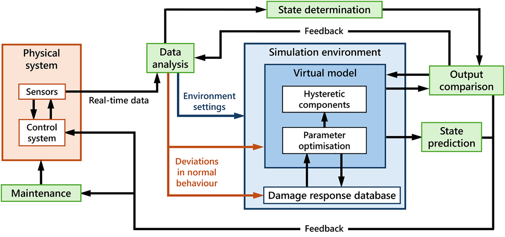
Figure 1: Digital twin system considering the hysteretic models

Since the simple models lack complexity, they may not provide sufficient data regarding the intricate real-world systems. Therefore, the authors implemented the hysteretic models into a simplified rail vehicle model with 7 DOF. The aim here is not to provide a complex description of a rail vehicle, but rather to utilise a more complex model serving as a base for the implementation and analysis of the hysteresis. Additionally, to include the stochastic nature of real-world conditions, the motion of the system is modelled as a stochastic process.

In the initial phase, the parameters for the nonlinear hysteresis models were calibrated to ensure comparable energy dissipation per loading cycle, analogous to the linear model. This calibration was performed by solving an optimisation problem using built-in MATLAB functions. Subsequently, the dynamic response of the railway vehicle’s vertical vibrations, kinematically induced by track irregularities, was analysed. The vertical irregularities of each track were modelled using the Kanai-Tajimi differential filter, which modulates white noise based on a specified power spectral density (PSD). The modelling process accounted for variable railway vehicle speed. The railway vehicle was modelled as a system of three rigid bodies with seven degrees of freedom, and the equations of motion were supplemented by eight additional control equations describing the hysteretic suspension elements. This system of differential equations was solved numerically using MATLAB’s ode45 function. The results obtained from the nonlinear models were statistically analysed and compared with those of the reference linear model. Furthermore, the impact of hysteresis models on the system’s frequency response was evaluated via the power spectral density of the solution corresponding to each model.

2  Introduction to the Mathematical Modelling of Hysteretic Behaviour in Engineering Systems

The following section presents the utilised hysteretic models. The typical loop shapes and governing equations are described. The section also deals with the process of finding desired parameters for each hysteretic model, based on the equivalent energy dissipation per loading cycle criteria.

2.1 Overview of Hysteresis Models

This study primarily focuses on five selected hysteresis models and their applications. Specifically, the bilinear model and several smooth models of the Bouc–Wen type are considered, including the standard Bouc–Wen model, the asymmetric Wang–Wen model, and the generalised Bouc–Wen model. Their performance is compared against a reference linear model.

2.1.1 Linear Model

Consider a linear elastic element characterised by a constant stiffness k and a viscous friction coefficient b. The total hysteretic force, FL, is expressed as the sum of the elastic restoring force Fk and the damping force Fb:

FL=Fk+Fb=kδ+bδ˙,(1)

where δ and δ˙ denote the displacement and its time derivative of the elastic element, respectively. The damping component Fb=bδ˙ accounts for hysteresis, with the area of the hysteresis loop being proportional to the coefficient b. In this case, hysteresis has an elastic character, as the system returns to its initial state without residual deformations upon unloading. The hysteresis loop describing the behaviour of the linear model is illustrated in Fig. 2a.

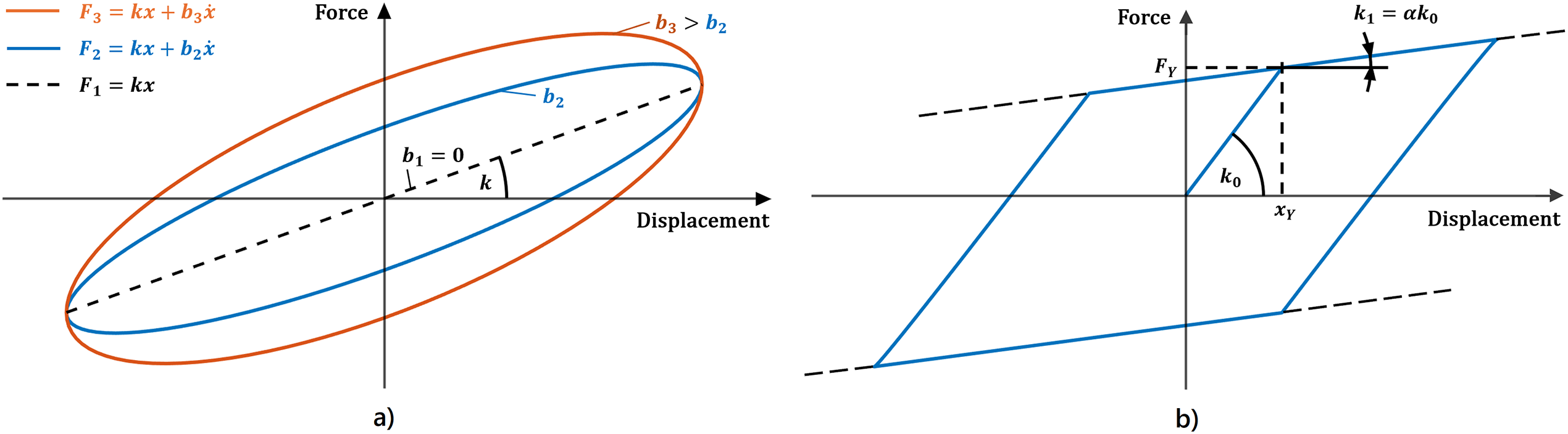
Figure 2: (a) Hysteresis loops for the linear model; (b) Hysteresis loop for the bilinear model

In the case of nonlinear hysteresis models, the total hysteresis force may be expressed as [3,6]:

FH=αkδ+(1−α)kz,(2)

where α generally denotes the stiffness ratio, k is the initial stiffness, and z represents the hysteretic control function. The term αkδ corresponds to the linear component of the force, while the remaining part of the expression represents the nonlinear hysteretic component. In this context, it is assumed that energy dissipation occurs solely due to the system’s hysteretic behaviour. Therefore, damping is not explicitly included in Eq. (2).

For the hysteretic models considered in this study, the control function z is defined exclusively in its differential form z˙. This differential form is specific to each hysteretic model. For each hysteretic element, this form corresponds to an additional differential equation, which is solved concurrently with the system of equations of motion.

2.1.2 Bilinear Model

The bilinear hysteresis model is characterised by a hysteresis loop exhibiting a sudden change in stiffness upon exceeding the yield limit. The differential form of the control function z=zBL can be expressed as follows:

z˙BL(δ˙,zBL)=δ˙2{1+sgn[xy−zBLsgn(δ˙)]}.(3)

The initial change in stiffness arises after surpassing the yield force FY, which corresponds to the displacement xY. The hysteretic force is expressed in the form of Eq. (2), incorporating both the initial stiffness k=k0=FY/xY and the post-yield stiffness k1=αk0. The hysteresis loop of the bilinear model has a simple parallelogram shape; however, its flexibility can be enhanced by incorporating additional parameters into the shape function. The shape of the bilinear hysteresis loop is illustrated in Fig. 2b.

The remaining hysteresis models employed in this study are classified as smooth models, as they allow for a continuous variation of stiffness. In general, these models can be described by a control function expressed in differential form as:

z˙H=(A−|zH|nψ).(4)

The constant A allows further modification of the initial slope of the hysteresis loop, which corresponds to the initial stiffness of the model. Meanwhile, the parameter n controls the sharpness of the loop. The shape function ψ is defined by the specific smooth model employed, with the flexibility of the hysteresis loop’s form depending on the complexity and number of parameters involved. The three smooth models considered in this study are the Bouc-Wen model, the asymmetric Wang-Wen model, and the generalised Bouc-Wen model.

2.1.3 Bouc-Wen Model

The shape of the hysteresis loop in the Bouc-Wen model is determined by the control function zH=zBW, expressed in differential form as shown in Eq. (4). This model defines the shape function ψBW by the following relation [3,6]:

ψBW(δ˙,zBW)=γ+βsgn(δ˙zBW).(5)

The sum and difference of the constants γ+β and γ−β define the values of the shape function ψBW, which control the changes in slope of the hysteresis loop across its various segments. From Eq. (5), it is evident that the function ψBW attains two distinct values ψ1 and ψ2, which can be determined from the following system of equations:

(111−1).(γβ)=(ψ1ψ2).(6)

The shape of the Bouc-Wen hysteresis loop is depicted in Fig. 3a.

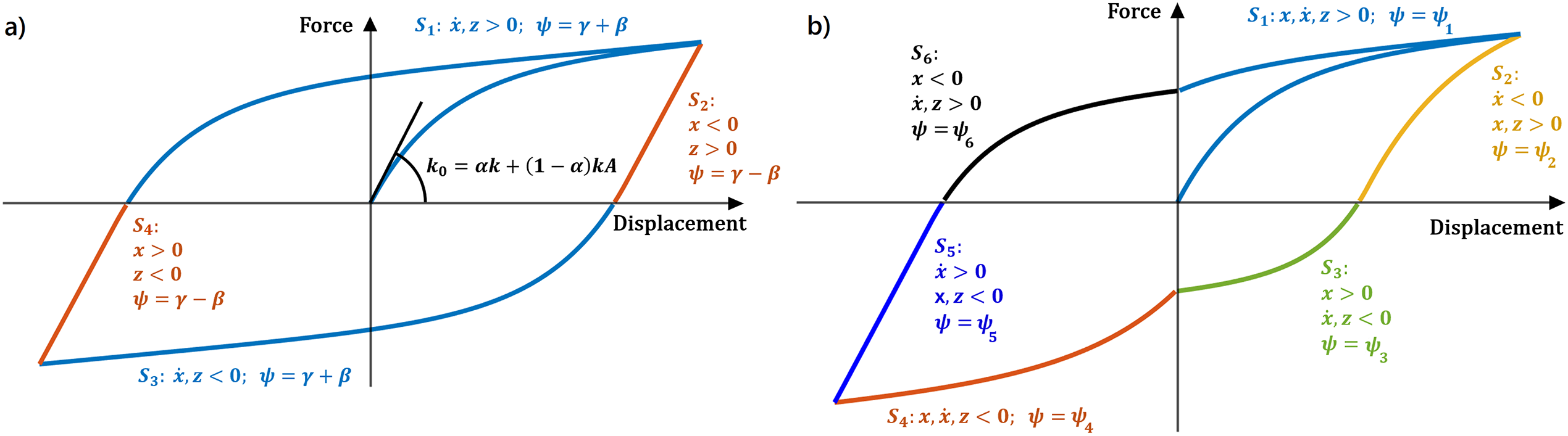
Figure 3: (a) Description of the hysteresis loop segments for the Bouc-Wen model; (b) Hysteretic loop for the generalised model

2.1.4 Asymmetric Wang-Wen Model

A further model considered, the Wang-Wen model, is formally an extension of the Bouc-Wen model with an added parameter φ that controls the asymmetry of the loop. Its shape function is expressed as [3]:

ψWW(δ˙,zWW)=γ+βsgn(δ˙zWW)+φ[sgn(δ˙)+sgn(zWW)].(7)

The roles of parameters β and γ remain consistent with the Bouc-Wen model, while the control function zH=zWW retains the differential form given by Eq. (4). From Eq. (7), it is evident that the value ψWW, which controls the degree of slope change in the loop, is increased by 2φ for positive displacement rates δ˙,z>0 and decreased by 2φ for negative displacement rates δ˙,z<0. Consequently, this enables different maximum values of the hysteretic force for positive and negative displacements δ. Asymmetric loops generated by the Wang-Wen model are illustrated in Fig. 4.

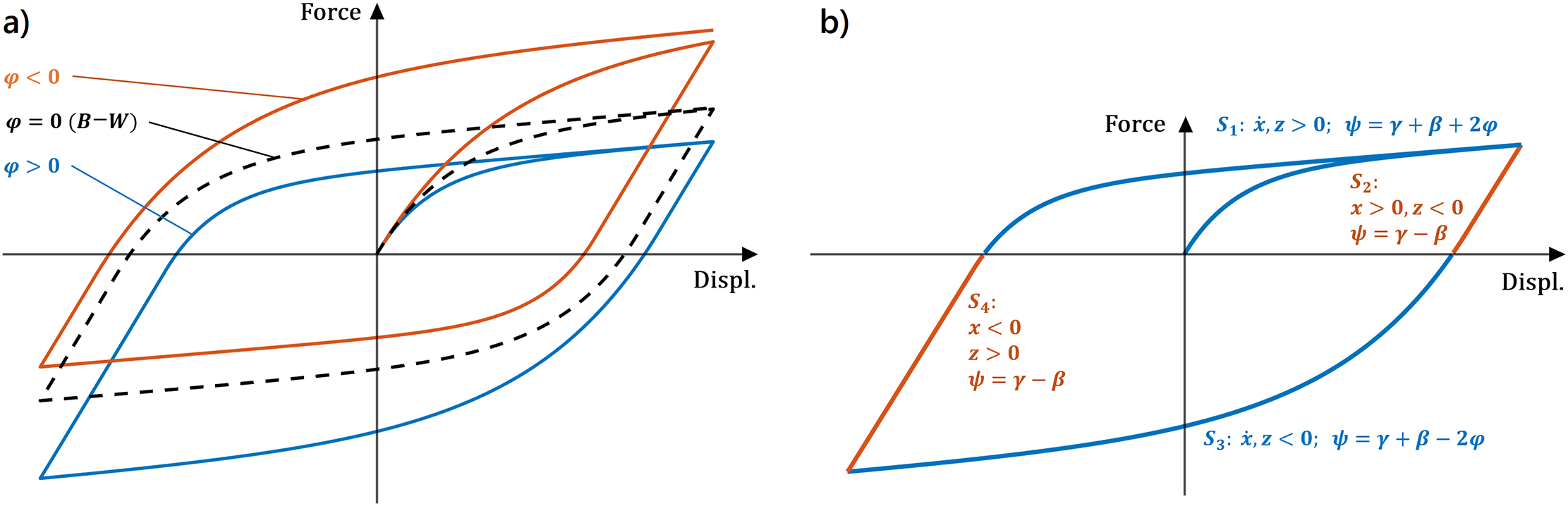
Figure 4: (a) Hysteresis loops for varying values of parameter φ; (b) Description of the individual segments in a Wang-Wen-type loop

In this case as well, the targeted values ψ1,ψ2,ψ3, attained by the shape function ψWW, can be determined by solving the corresponding linear system of equations:

(1121−1011−2).(γβφ)=(ψ1ψ2ψ3).(8)

2.1.5 Generalized Bouc-Wen Model

The generalized Bouc-Wen model, which we consider as the final smooth model in this study, uses a six-parameter shape function ψGBW. This function specifies distinct slope variations across each of the six segments of the hysteresis loop, with segments defined by the signs of the state variables δ,δ˙ and z.

The slope in each segment can be independently controlled, providing a high degree of flexibility in the loop shape. Consequently, this model can capture strongly asymmetric hysteretic behaviours. The shape function of this model is expressed as follows [3]:

ψGBW(δ,δ˙,zGBW)=[ sgn(δ˙zGBW)+sgn(δδ˙)+sgn(δzGBW)+sgn(δ)+sgn(δ˙)++sgn(zGBW)]⋅βGBW.(9)

The vector βGBW=[β1,…,β6]T contains the parameters controlling the shape of the hysteresis loop, and the values of these constants (β1,…,β6) are determined by solving the following system of equations [1]:

(111111−11−11−11−1−111−1−1111−1−1−1−11−1−11−1−1−11−111).(β1β2β3β4β5β6)=(ψ1ψ2ψ3ψ4ψ5ψ6).(10)

The constants ψ1,…,ψ6 correspond to the required values of the shape function ψGBW, in the respective segments of the hysteresis loop, as illustrated in Fig. 3b.

2.2 Computational Parameters for Hysteresis Models

As previously stated, in nonlinear hysteretic systems, damping, consequently, energy dissipation is regarded as a direct consequence of the hysteretic effect. Therefore, the parameters of the hysteretic models were selected to ensure that their behaviour, in terms of energy dissipation, remains approximately equivalent. As a result, we defined the primary criterion for comparison as the amount of energy dissipated per loading cycle, as expressed by the following relation:

WD=∫t1t2Fδ˙dt.(11)

The considered cycle is assumed to occur over the time interval ⟨t1;t2⟩, where F denotes the total hysteretic force and δ˙ represents the displacement rate of the elastic element. The energy dissipated over the cycle is equivalent to the area enclosed by the corresponding hysteresis loop.

The parameters of the nonlinear hysteresis models were determined through an optimisation procedure solved in MATLAB, using the fminsearch function. This optimisation aimed to ensure that the energy dissipated during a loading cycle in the nonlinear models closely approximates that of a reference linear model. This condition was enforced across the 24 symmetric loading cycles, with amplitudes ranging within the interval ⟨0.5;12⟩ mm.

2.2.1 Linear Model

For the reference linear model, the hysteretic force is given by Eq. (1). This study deals with a rail vehicle model, which will be presented later. The model contains two types of suspension components with different parameters. Thus, two groups of hysteretic elements, denoted as group A and B, are considered. Group A is characterised by parameters k1,b1, while the group B is defined by parameters k2,b2. The parameters of the nonlinear models were determined separately for each group (A,B). For the nonlinear models, the hysteretic force is expressed by Eq. (2), with each model further described by its control function z˙in differential form.

2.2.2 Bilinear Model

In the bilinear model, the shape of the hysteresis loop is prescribed by the control function z˙BL in the form of Eq. (3). Among the optimisation variables, the parameter xy, which determines the value of the control function zBL at which the abrupt change in stiffness occurs was selected. In addition, the parameter k=kBL defining the initial stiffness and the parameter α=αBL representing the stiffness ratio were also optimised. These parameters are incorporated in Eq. (2). The subsequent smooth models are further characterised by specific shape functions ψ, which form part of the control function defined in Eq. (4).

2.2.3 Bouc-Wen Model

The Bouc-Wen model is defined by the shape function presented in Eq. (5). The parameters β=βBW and γ=γBW controlling the shape of the hysteresis loop were considered as an optimisation variables. Additionally, a parameter n=nBW, influencing the sharpness of the loop, and parameters α=aBW and k=kBW, whose significance is analogous to those in the bilinear model, were included in Eqs. (2) and (4). For each smooth model, the value of A=1 was specified.

2.2.4 Wang-Wen Model

The shape function for the Wang-Wen model is defined by Eq. (7), where the parameters β=βWW and γ=γWW were optimised along with the parameter φ, which controls the asymmetry of the hysteresis loop. As in the previous case, the parameters α=αWW, k=kWW and n=nWW in Eqs. (2) and (4) were also subjected to optimisation.

2.2.5 Generalised Bouc-Wen Model

In the optimisation of the generalised Bouc-Wen model, a modified shape function was employed:

ψGBW=[sgn(δ˙zGBW)+sgn(δδ˙)+sgn(δzGBW)+sgn(δ)+sgn(δ˙)+sgn(zGBW)]⋅K βGBW.(12)

The constant K  appears in the given function solely as an additional parameter and, together with the parameters k=kGBW, α=αGBW and n=nGBW constitutes part of the optimisation variables. In contrast, the elements of the vector βGBW are not subject to optimisation to preserve the prescribed shape of the hysteresis loop.

2.2.6 Optimisation Results

An overview of the optimisation results is presented in Fig. 5, which displays, for each hysteresis model, the area enclosed by the hysteresis loop as a function of the loading cycle amplitude. The maximum displacement of suspension components that occurred in the linear model was approximately 10 mm. Therefore, the optimisation was carried out for a set of 24 amplitudes ranging from 0.5 mm to 12 mm.

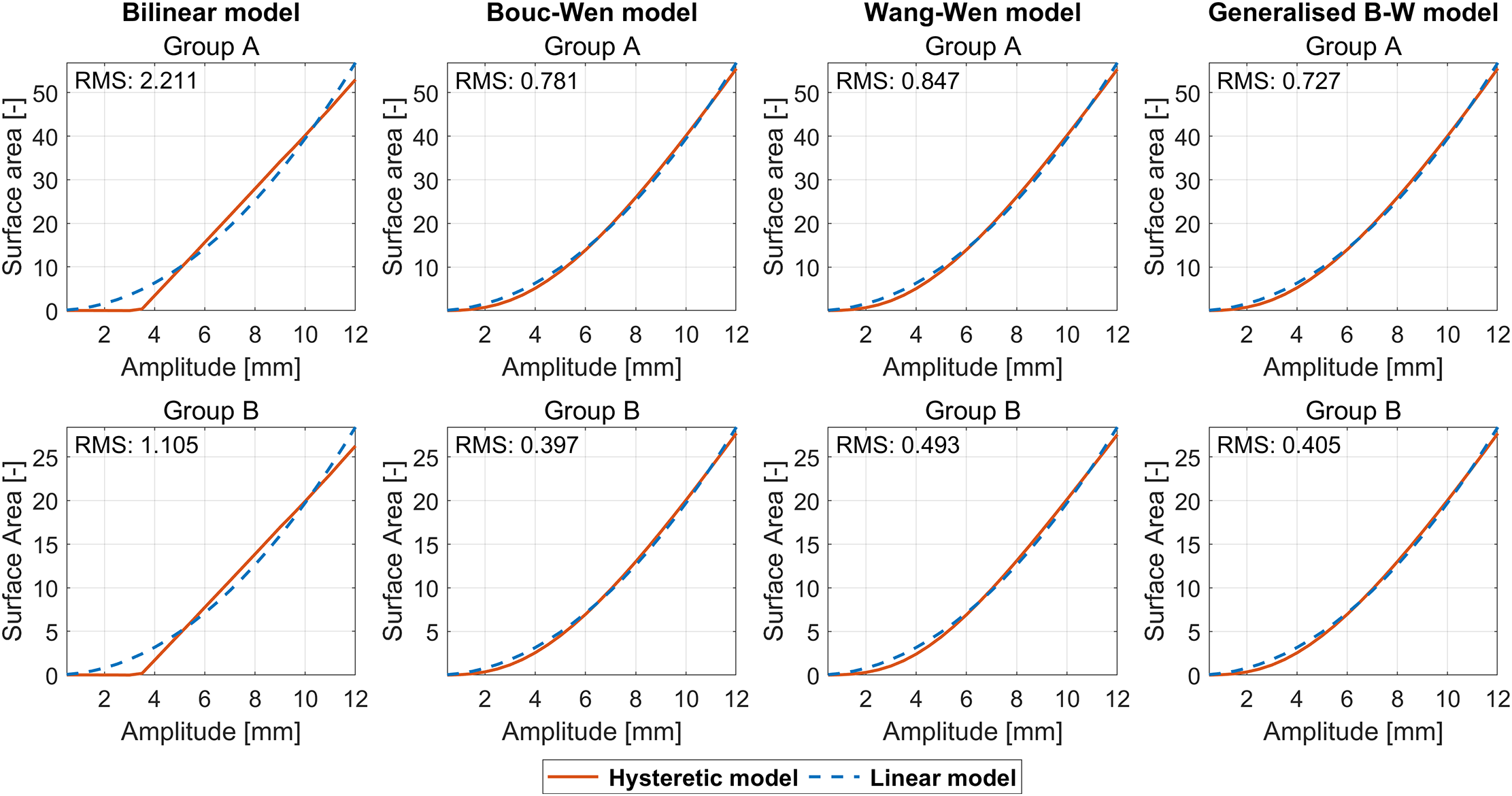
Figure 5: Optimisation results of hysteresis models

Additionally, the root-mean-square (RMS) differences between the loop areas of the respective nonlinear models and the reference linear model are provided.

Considering these RMS differences, the largest discrepancies were observed for the bilinear model across both groups of elements (A and B). This outcome can be attributed to the relatively low flexibility of the bilinear model in comparison to the other nonlinear models. Furthermore, the graphs reveal a bilinear dependence between the hysteresis loop area and the loading cycle amplitude for this model.

The remaining nonlinear models provide a closer approximation to the reference model, producing mutually comparable results. This observation is supported by both the graphical representations in Fig. 5 and the corresponding RMS values. Among these models, the generalised Bouc-Wen model has the smallest discrepancies despite having the fewest optimisation variables. These findings are consistent for both groups of elastic elements (A and B).

3  Evaluation of the Implementation Feasibility of Hysteresis Models in Railway Vehicle Dynamics

The following section focuses on the integration of the previously discussed hysteresis models into a mathematical model of a railway vehicle. The vehicle under consideration consists of a wagon body and two single-axle bogies, interconnected by spring elements exhibiting hysteretic stiffness properties. The vehicle travels at a variable speed along a railway track, undergoing vertical vibrations induced by track irregularities. The primary aim of this study is not to present a comprehensive railway vehicle model but rather to demonstrate the application of selected hysteresis models within the context of railway vehicle dynamics.

3.1 Physical Model of the Vehicle

The vehicle is modelled as a system of three rigid bodies representing the wagon body and the individual bogies. Two groups of suspension elements provide the elastic connections between these bodies.

The group A (suspensions P1 to P4) connects the wagon body to each bogie, while group B (suspensions P5 to P8) connects the bogies to their respective wheelsets. These wheelsets are not modelled as independent rigid bodies; rather, only the vertical displacements of individual wheels are considered, with their motion representing the kinematic excitation of the vehicle. The described model is illustrated in Fig. 6.

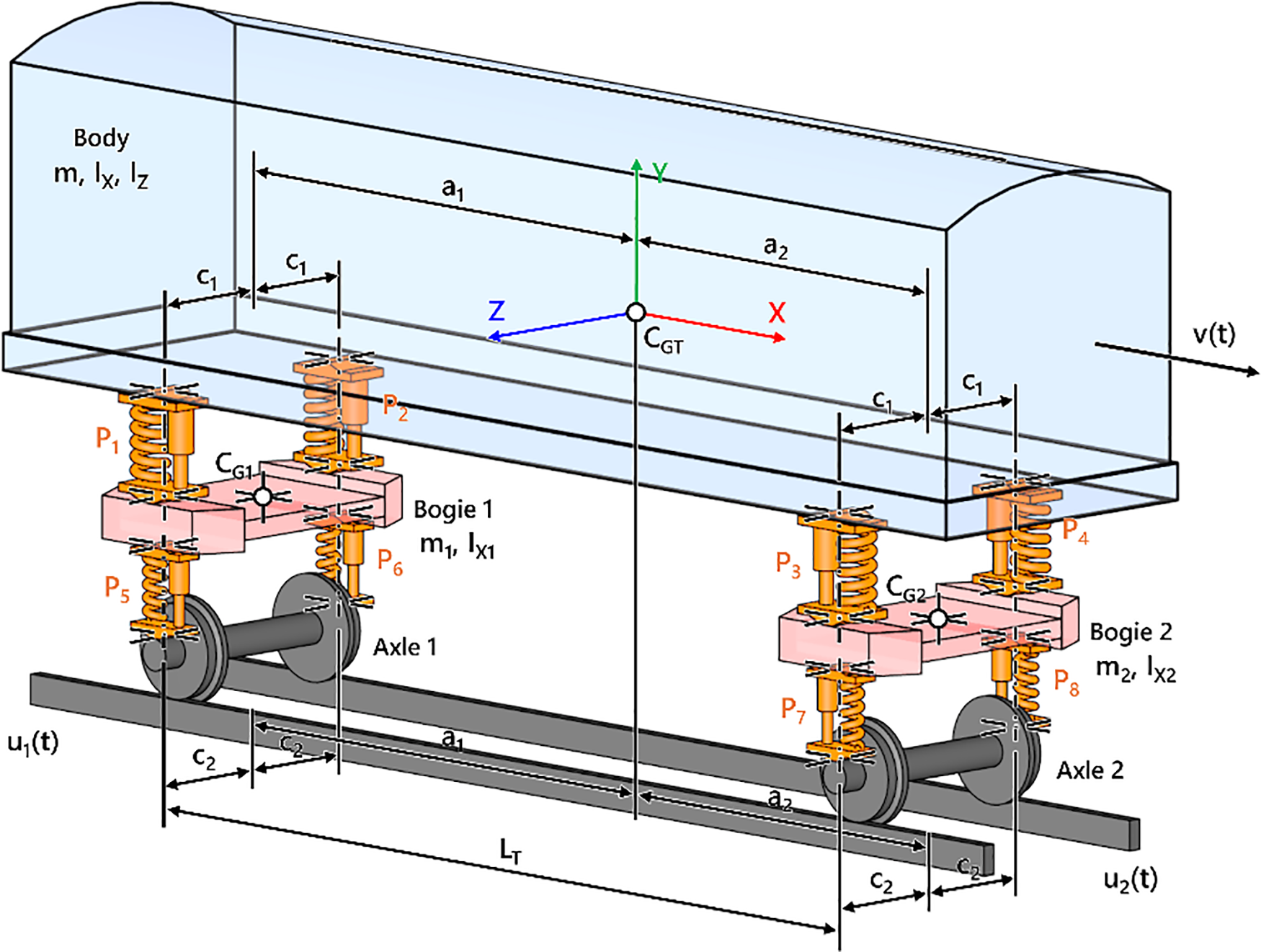
Figure 6: The physical model of the railway vehicle

The system possesses a total of seven degrees of freedom (DOF). For the wagon body, the model considers the vertical displacement yC and rotations about the longitudinal and lateral axes, denoted as φCX, φCY. For each bogie, the corresponding vertical displacements y1,y2 and rotations φ1X,φ2X about the longitudinal axis X are included. A known time-dependent function defines the motion of the wheelsets; therefore, the system does not incorporate this motion into its degrees of freedom.

The distance between the bogies is denoted by L=24.5 m, where a1=12 m and a2=12.5 m represent the longitudinal distances of the bogie centres of gravity from the centroid of the wagon body along the X axis. The dimensions c1=c2=1 m define the lateral positions along the bogies where the suspension springs are attached. The body mass is mC=16,100 kg, and its moments of inertia about the longitudinal and lateral axes are represented by JCX=13,700 kg⋅m2 and JCZ=787,570 kg⋅m2. Each bogie has a mass m1=m2=3050 kg and a moment of inertia about its vertical X axis J1X=J2X=1230 kg⋅m2 (Fig. 6). Given the nature of the vehicle motion under consideration, the moments of inertia about the remaining axes are neglected.

The vehicle velocity is prescribed by a piecewise-defined function, with its temporal profile shown in Fig. 7. This function consists of three constant segments smoothly connected via cosine-based transitions. The initial and final velocities both have the value v0=10 m/s V, while the maximum velocity attained by the vehicle is vM=25 m/s. Due to the variable velocity, the phase shift P between the individual wheelsets is computed at each time step based on the travelled distance.

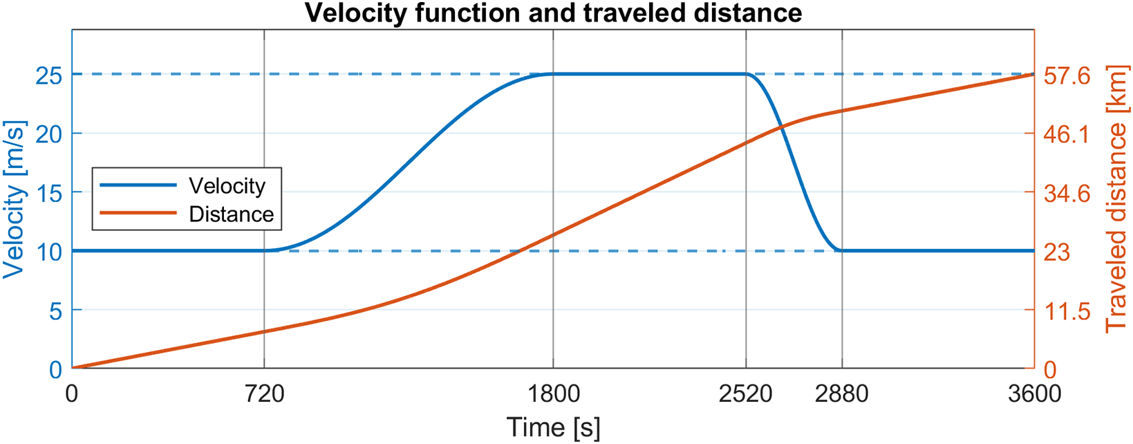
Figure 7: Temporal profile of vehicle velocity and travelled distance

The vehicle vibration is excited kinematically by functions u1(t),u2(t), describing the vertical displacements of individual wheels over time. Each of these functions, representing vertical irregularities of the respective track, is modelled as a stochastic time-dependent function using the Kanai-Tajimi differential filter. The detailed methodology for generating these excitation functions will be presented in a subsequent section.

3.2 Mathematical Model

The free-body diagram of the vehicle is depicted in Fig. 8. The hysteretic forces acting within the suspension elements are highlighted in orange, while the displacements corresponding to the kinematic excitation are indicated in blue. Coordinates defining the positions of individual components are marked in red. Considering hysteretic suspension, the total hysteretic force in the i-th suspension element can be expressed as:

FHi=αikiδi+(1−αi)kizi+biδ˙i,for i=1,2,…,8.(13)

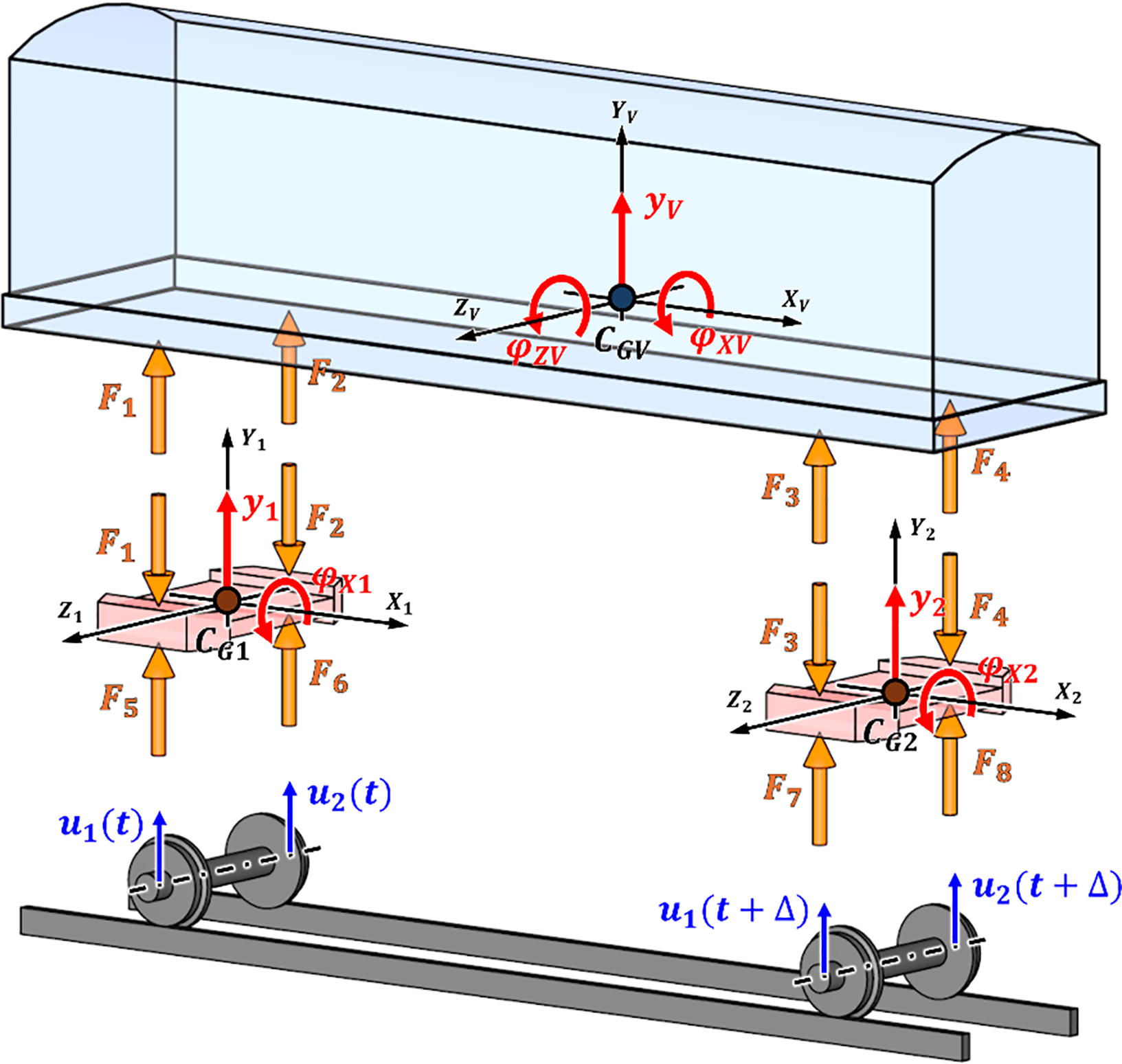
Figure 8: Free-body diagram of the model

The quantity δi denotes the displacement of the elastic element, and δ˙i represents the time derivative of this displacement. To facilitate the formulation of the subsequent equations of motion, the damping force biδ˙i is explicitly included in the analysis.

Assuming small displacements and rotations, the problem can be treated as geometrically linear. Consequently, the displacements of individual elements and their corresponding time derivatives can be expressed in vector form as:

δ=D⋅x,δ˙=D⋅x˙.(14)

The displacement vector and its time derivative are expressed as: δ=(δ1,…,δ8)T, δ˙=(δ˙1,…,δ˙8)T. The displacements and rotations vector is: x=[ y φZ φX y1 φX1 y2 φX2 u1(t) uΔ1(t) u2(t) uΔ2(t) ]T and analogously x˙=[y˙ ⋯ u˙Δ2(t)]T. The matrix D is defined as:

D=(1−a1−c1−1c10000001−a1c1−1−c10000001a2−c100−1c100001a2c100−1−c100000001−c200−10000001c2000−100000001−c200−10000001c2000−1)8×11(15)

where ai and ci correspond to the dimensions specified in Fig. 6.

Considering the forces (13) and (14), a system of 15 differential equations can be formulated, representing the mathematical model of the vehicle:

mCy¨C=−kα1δ1−(1−α1)k1z1−kα2δ2−(1−α2)k2z2−kα3δ3−(1−α3)k3z3−

−kα4δ4−(1−α4)k4z4−b1δ˙1−b2δ˙2−b3δ˙3−b4δ˙4,

JZCφ¨ZC=a1[kα1δ1+(1−α1)k1z1+kα2δ2+(1−α2)k2z2]−a2[kα3δ3+(1−α3)k3z3+

+kα4δ4+(1−α4)k4z4]+a1[b1δ˙1+b2δ˙2]−a2[b3δ˙3+b4δ˙4],

JXCφ¨XC=c1[kα1δ1+(1−α1)k1z1+kα3δ3+(1−α3)k3z3−kα2δ2−(1−α2)k2z2−

−kα4δ4−(1−α4)k4z4]+c1[b1δ˙1+b3δ˙3−b2δ˙2−b4δ˙4],

m1y¨1=kα1δ1+(1−α1)k1z1+kα2δ2+(1−α2)k2z2−kα5δ5−(1−α5)k5z5−

−kα6δ6−(1−α6)k6z6+b1δ˙1+b2δ˙2−b5δ˙5−b6δ˙6,

JZ1φ¨Z1=c1[kα2δ2+(1−α2)k2z2−kα1δ1−(1−α1)k1z1]+c2[kα5δ5+(1−α5)k5z5−

−kα6δ6−(1−α6)k6z6]+c1[b2δ˙2−b1δ˙1]+c2[b5δ˙5−b6δ˙6],

m2y¨2=kα3δ3+(1−α3)k3z3+kα4δ4+(1−α4)k4z4−kα7δ7−(1−α7)k7z7−

−kα8δ8−(1−α8)k8z8+b3δ˙3+b4δ˙4−b7δ˙7−b8δ˙8,

JZ2φ¨Z2=c1[kα4δ4+(1−α4)k4z4−kα3δ3−(1−α3)k3z3]+c2[kα7δ7+(1−α7)k7z7−

−kα8δ8−(1−α8)k8z8]+c1[b4δ˙4−b3δ˙3]+c2[b7δ˙7−b8δ˙8].

z˙i=Ψi(δi,δ˙i,zi),fori=1,2,…,8.(16)

The first seven equations of system (16) represent the equations of motion of the vehicle, for which the following relation holds kαi=αiki. The remaining part of the system consists of additional equations for the control functions of hysteresis zi,whose specific forms Ψi depends on the chosen hysteresis model. For the bilinear model, these functions have the form:

z˙i=δ˙i2{1+sgn[xy−zisgn(δ˙i)]},fori=1,2,…,8.(17)

Smooth hysteretic models are then described by control functions of the form:

z˙i=[Ai−|zi|niψi]δ˙i,fori=1,2,…,8.(18)

The individual smooth models also differ in their respective shape function equations ψi, as defined by Eqs. (5), (7) and (9).

By neglecting all terms (1−αi)kizi in Eq. (16) and setting αi=1, a linear system of equations is obtained, representing the reference linear model. Consequently, all additional equations of the form z˙i=Ψi(δi,δ˙i,zi) become redundant, further simplifying the system under consideration. Conversely, for nonlinear hysteretic models, we assume bi=0, implying that energy dissipation occurs exclusively due to hysteretic effects.

System (16) was solved numerically in MATLAB using the ode45 function. The application of this method requires the system of differential equations to be expressed in first-order form (i.e., state-space representation), which necessitated the transformation of the first seven equations. As a result of this transformation, the nonlinear hysteretic models yield a system of 22 first-order differential equations, whereas the reference linear model results in a system comprising 14 equations.

3.3 Modelling of Random Kinematic Excitation Using the Kanai-Tajimi Differential Filter

The vertical vibration of the vehicle is excited by the functions u1(t), u2(t), each representing the temporal profile of vertical irregularities corresponding to a specific track. These functions were modelled as stochastic processes, with the Kanai-Tajimi differential filter employed.

The analysis begins with the consideration of the power spectral density of the track irregularity function u(t), the form of which is defined by ORE B 176, as follows [29,30]:

Su(Ω)=A⋅b2(Ω2+a2)(Ω2+b2),(19)

where a=0.0206 rad/m; b=0.8246 rad/m and A=4.032×10−7 rad⋅m for high-quality tracks and A=1.08×10−6 rad⋅m for lower-quality tracks. The power spectral density in Eq. (19) is shown in Fig. 9. The vehicle velocity v(t) was considered as a function of time Ω=ω/v, where ω denotes the angular frequency. Under this assumption, the Eq. (19) can be reformulated as a function of angular frequency and time [29]:

Su(ω,t)=1v(t)⋅A⋅b2[ω2v2(t)+a2][ω2v2(t)+b2].(20)

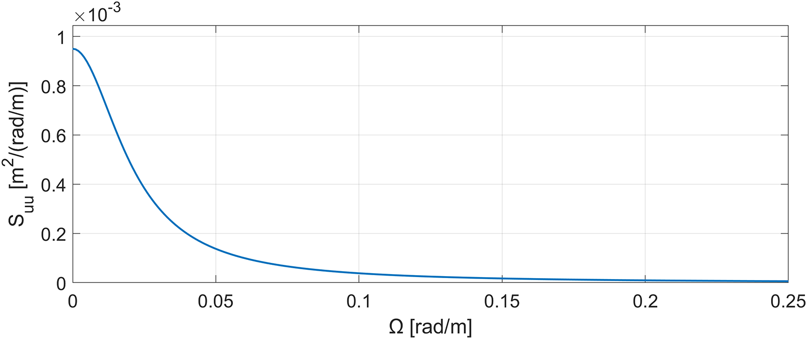
Figure 9: Power spectral density of the track irregularity function

The Kanai-Tajimi differential filter can be defined by the following equation:

meu¨(t)+beu˙(t)+keu(t)=w(t),(21)

where the parameters me, be and ke are unknown at this stage. The right-hand side w(t) denotes a Gaussian process with the characteristics of white noise and a constant power spectral density S0. The unknown parameters can be identified by comparing the spectral density from Eq. (20) with the frequency response function H(ω) of the filter, defined as [30]:

H(ω)=S0(ke−ω2me)2+ω2be2.(22)

By equating (20) to (22), assuming S0=1, we obtain the equation:

S0(ke−ω2me)2+ω2be2=1v(t)⋅A⋅b2[ω2v2(t)+a2][ω2v2(t)+b2].(23)

By comparing the same powers of ω: it is evident that:

me=14π2bv(t)Av(t),be=a+b2πbAv(t),ke=av(t)A(24)

If we rearrange and substitute the parameters from (24) to Eq. (21), we obtain:

Av(t)4π2Abv2(t)u¨(t)+(a+b)Av(t)2πAbv(t)u˙(t)+aAv(t)Au(t)=w(t).(25)

By solving the given equation with the initial conditions u(0)=u˙(0)=u¨(0)=0, the desired kinematic excitation function u(t) was obtained. This function was modelled separately for each track. In both cases, the parameter values were kept identical; however, different statistically equivalent Gaussian processes w1(t), w2(t)were generated. The resulting temporal profiles of the individual excitation functions (u1, u2) are shown in Fig. 10.

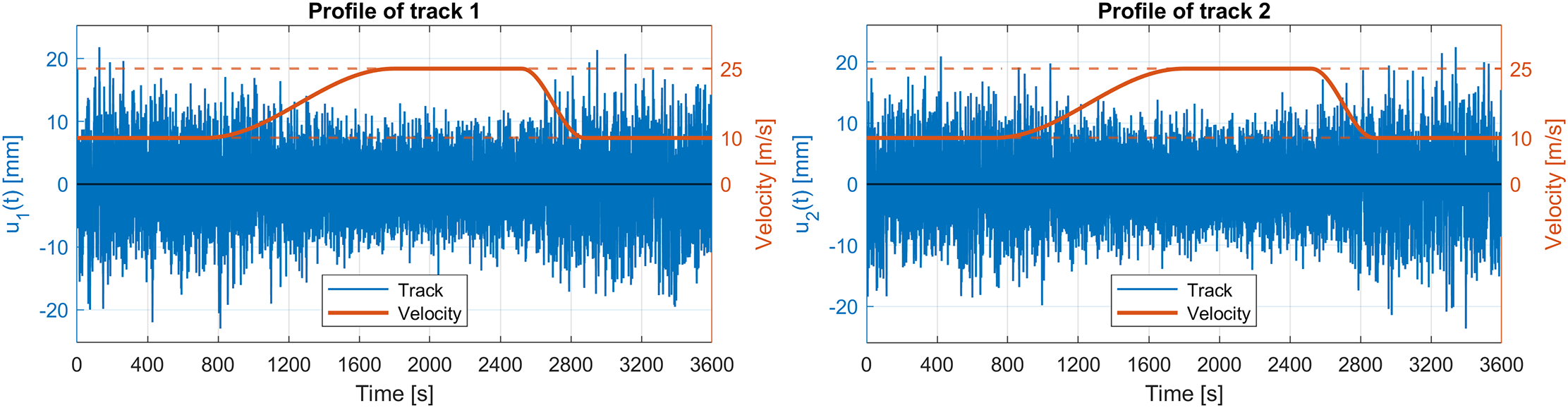
Figure 10: Temporal profiles of the kinematic excitation functions

The mean values of the presented excitation functions are u¯1=0.150 mm and u¯2=−0.089 mm, with corresponding standard deviations σ1=4.453 mm and σ2=4.367 mm.

4  Analysis of the Results in the Time Domain

The following sections present results in the time domain. For each hysteretic model, the results comprise the time courses for the body’s vertical displacement yC, the body rotation about the Z axis φZT (horizontal axis normal to the vehicle longitudinal axis) and the vertical displacements of each bogie, y1 (rear bogie), y2 (front bogie). The forces in suspension components (springs 3, 4—group A and 7, 8—group B) of the front axle were also studied. The results are presented in the form of hysteretic loops describing the force-displacement relationship in the suspension. Additionally, the time courses of the corresponding hysteretic forces are also shown. The statistical treatment of the results is presented in the following Section 4.1.

4.1 Linear Model

The time courses for the selected body and boogie coordinates are shown in Fig. 11. The hysteresis loops are presented in Figs. 12 and 13, together with the time courses of the respective hysteretic forces. Considering the presented results, the suspension components possess a relatively symmetric behaviour. The results for the components within the respective groups (A and B) are generally comparable. The displacements for group A are higher, with lower hysteretic forces, compared to the components of group B.

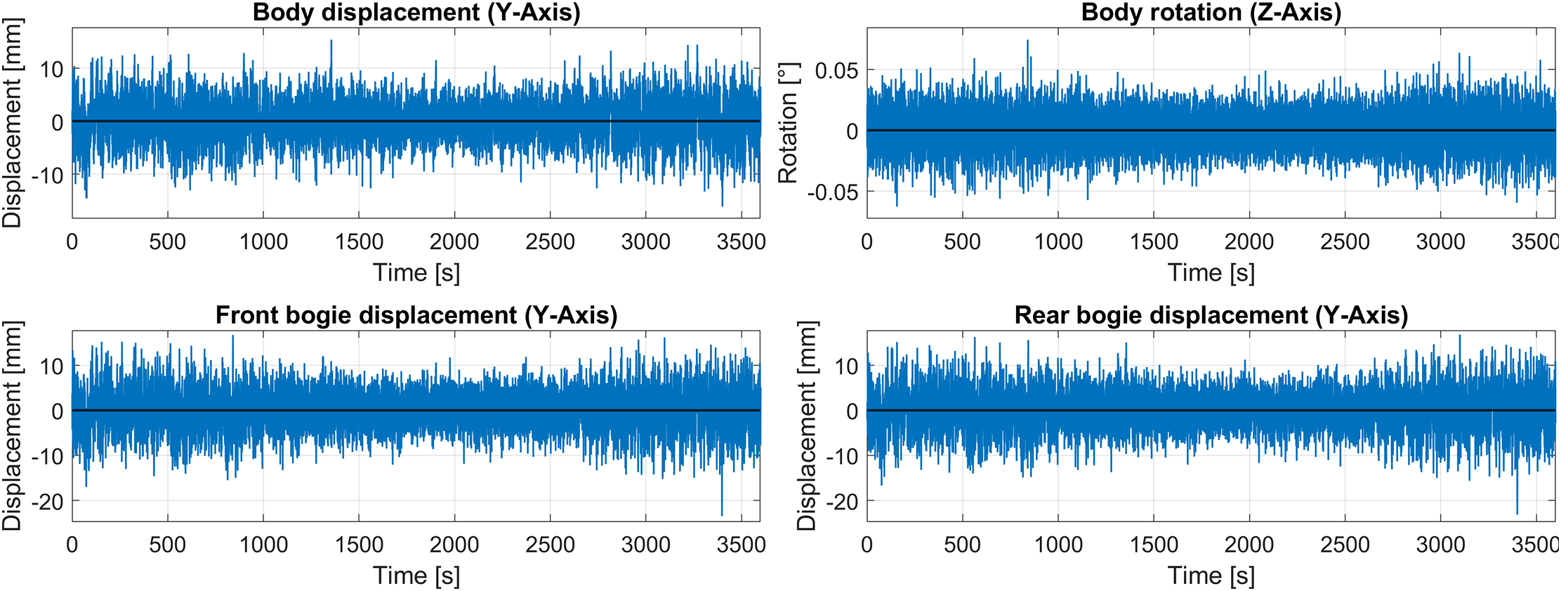
Figure 11: Response quantities for the linear model

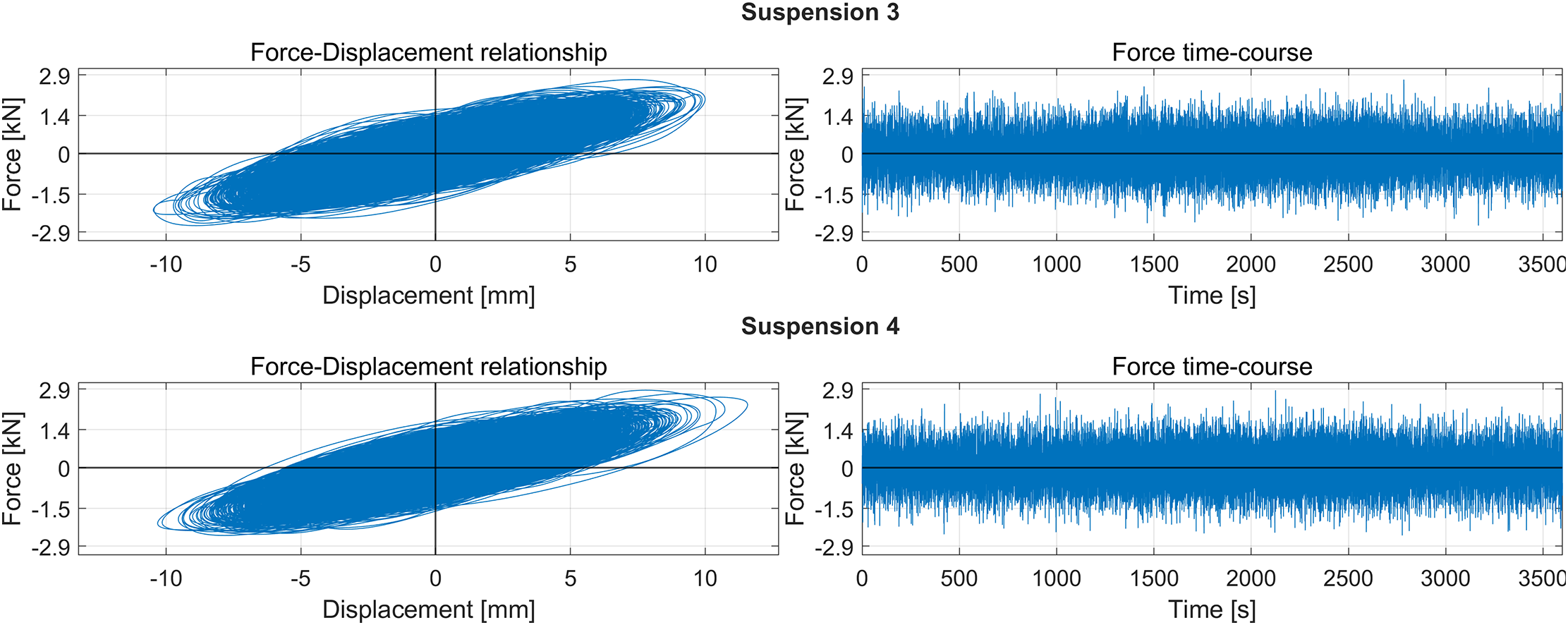
Figure 12: Hysteretic loops (left) and forces (right) for the linear model, suspension 3, 4

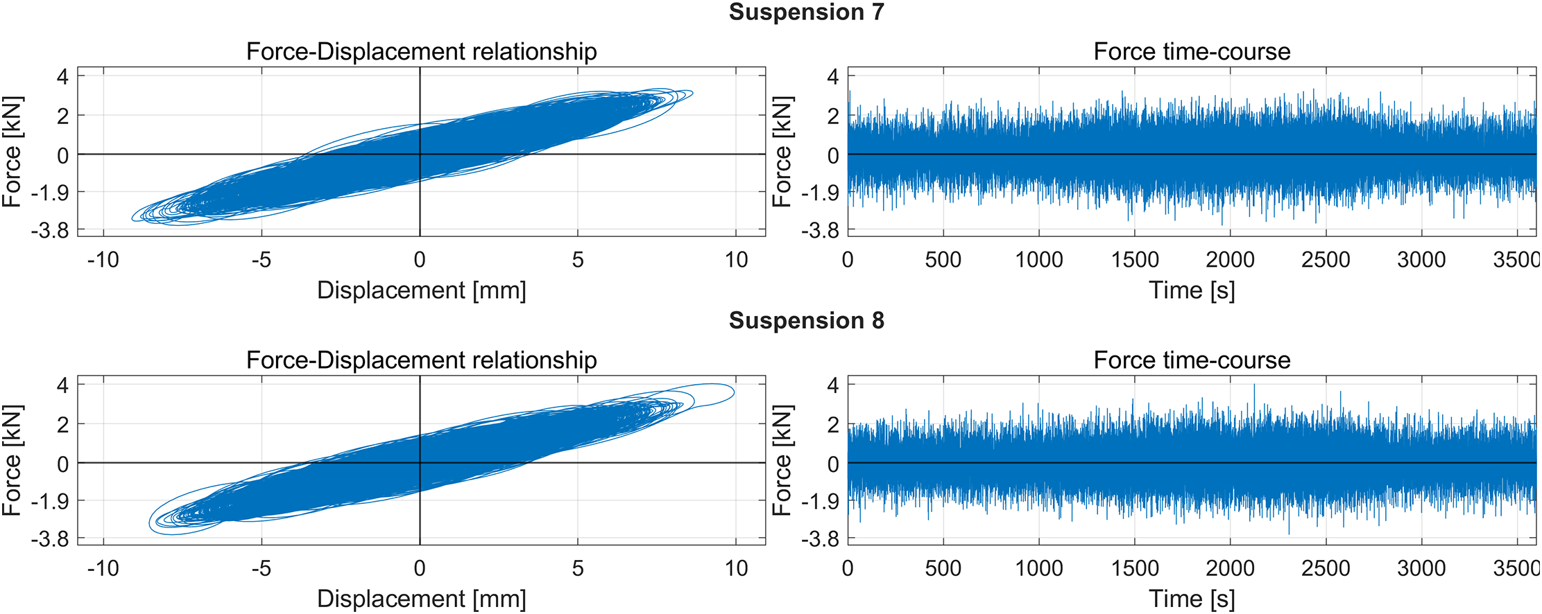
Figure 13: Hysteretic loops (left) and forces (right) for the linear model, suspension 7, 8

4.2 Bilinear Model

The response quantities for the bilinear model are shown in Fig. 14. The hysteretic loops and force time courses are presented in Figs. 15 and 16. Considering the loop shapes, the model again behaves symmetrically; however, the loops are no longer smooth. The behaviour of the suspension components within the respective group is again comparable. In this case, group A possesses both lower displacements and the maximum forces, compared to group B. The displacements in respective groups differ significantly compared to the previous case.

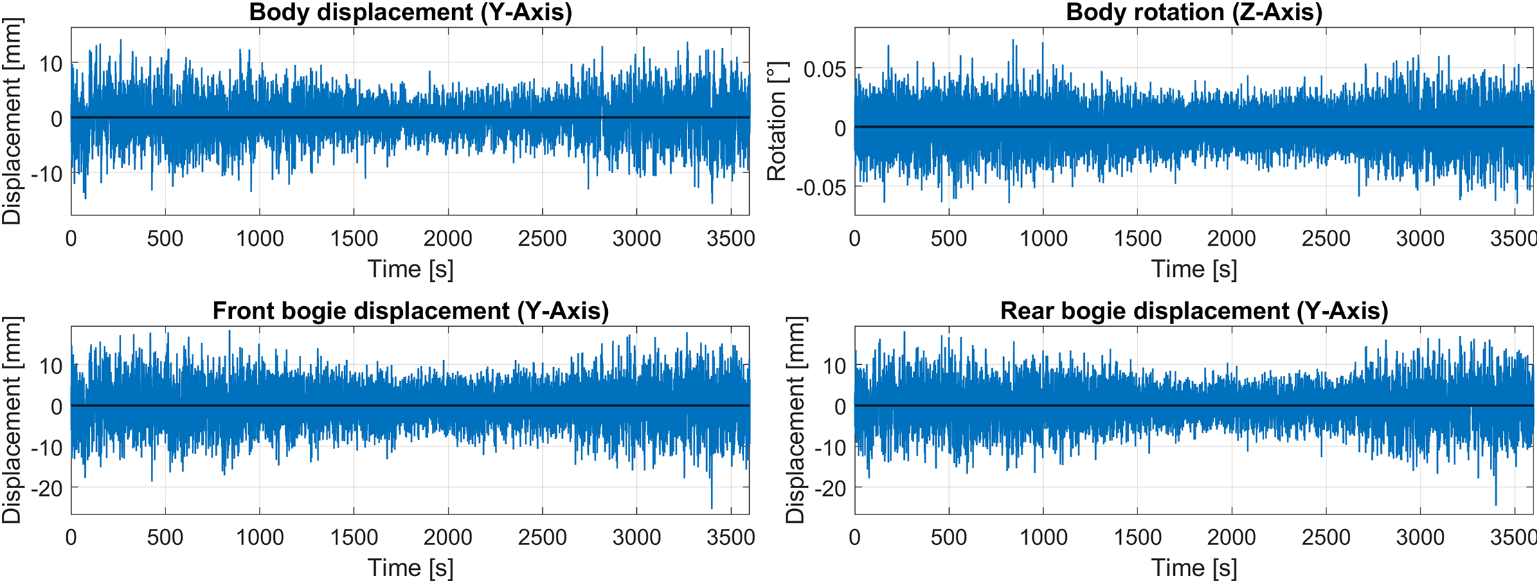
Figure 14: Response quantities for the bilinear model

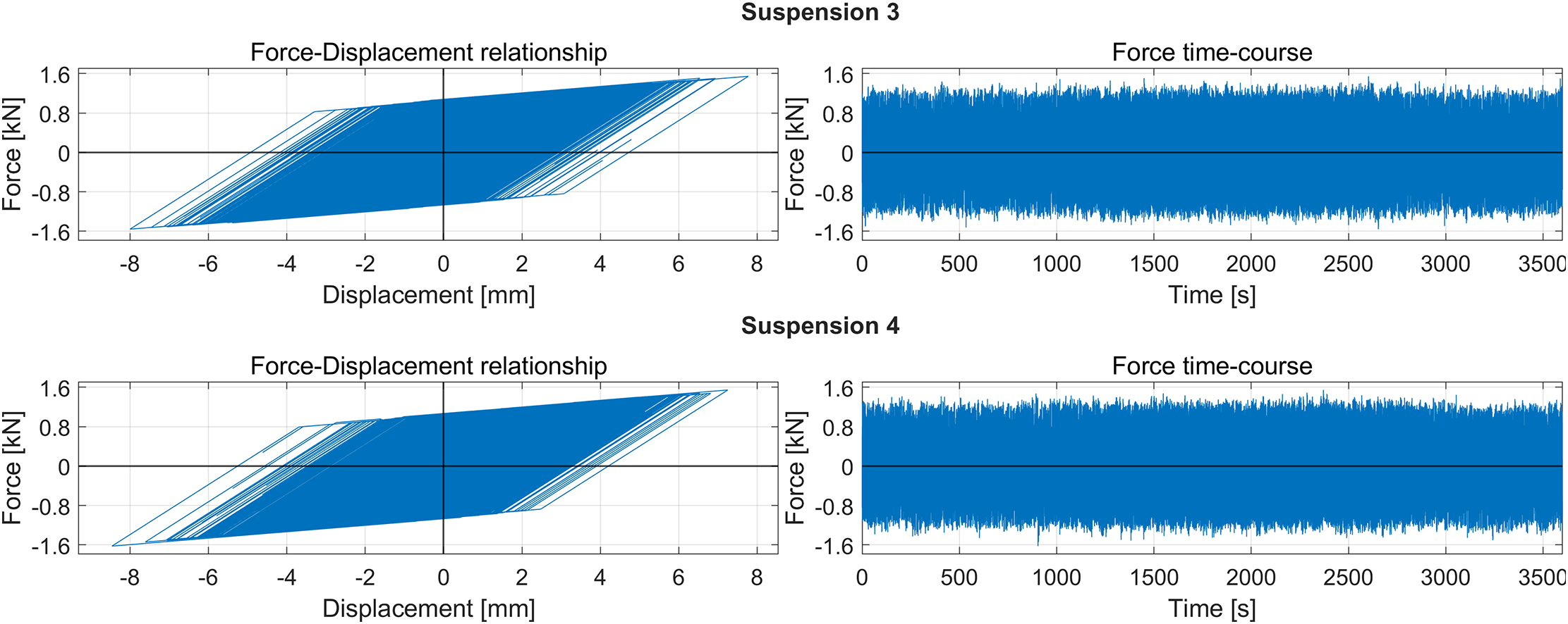
Figure 15: Hysteretic loops and force time courses for bilinear model, suspension 3, 4

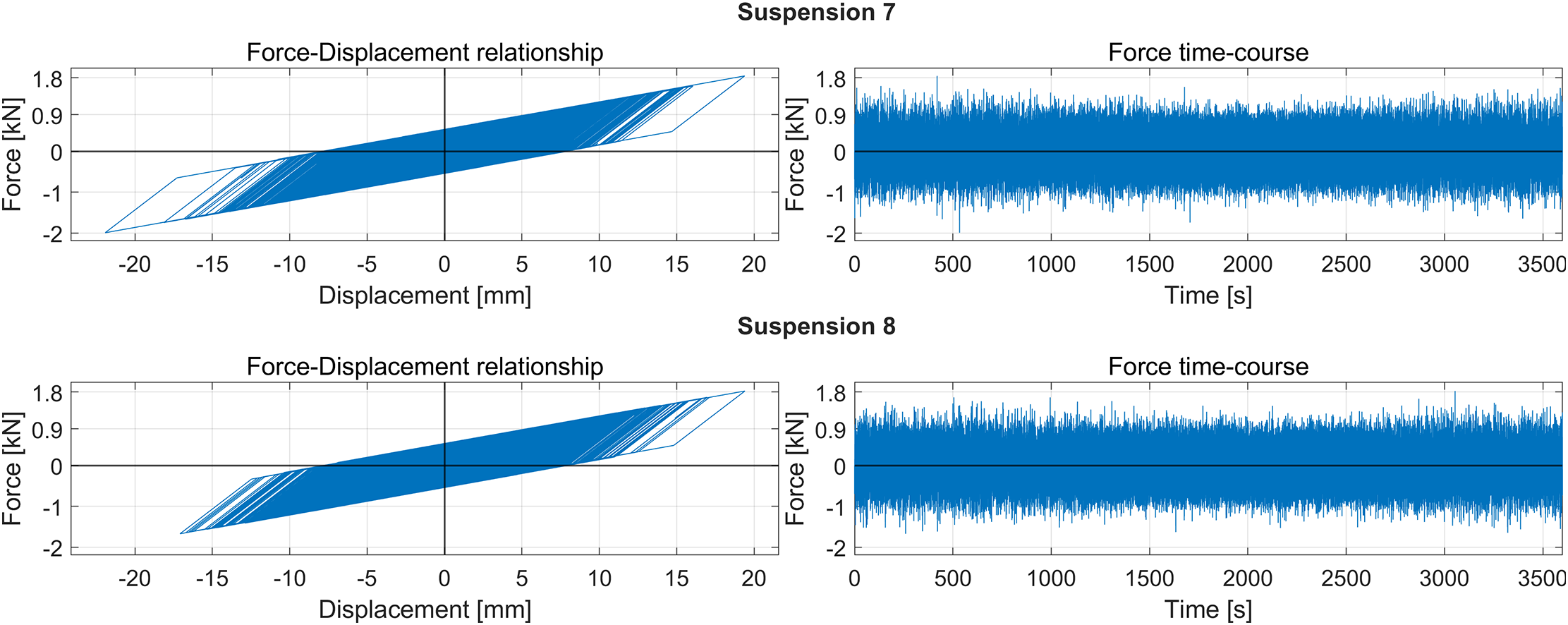
Figure 16: Hysteretic loops and force time courses for bilinear model, suspension 7, 8

4.3 Bouc-Wen Model

The response quantities are shown in Fig. 17 with the hysteretic loops and forces being shown in Figs. 18 and 19. As with the previous models, there is no noticeable asymmetry present in the hysteretic loop shapes. Again, the components within the respective groups exert comparable behaviour. In this case, the maximum forces are approximately the same in all components; however, group B achieves significantly higher displacements. Similarly to the previous case, this results in noticeably wider loops for group B components.

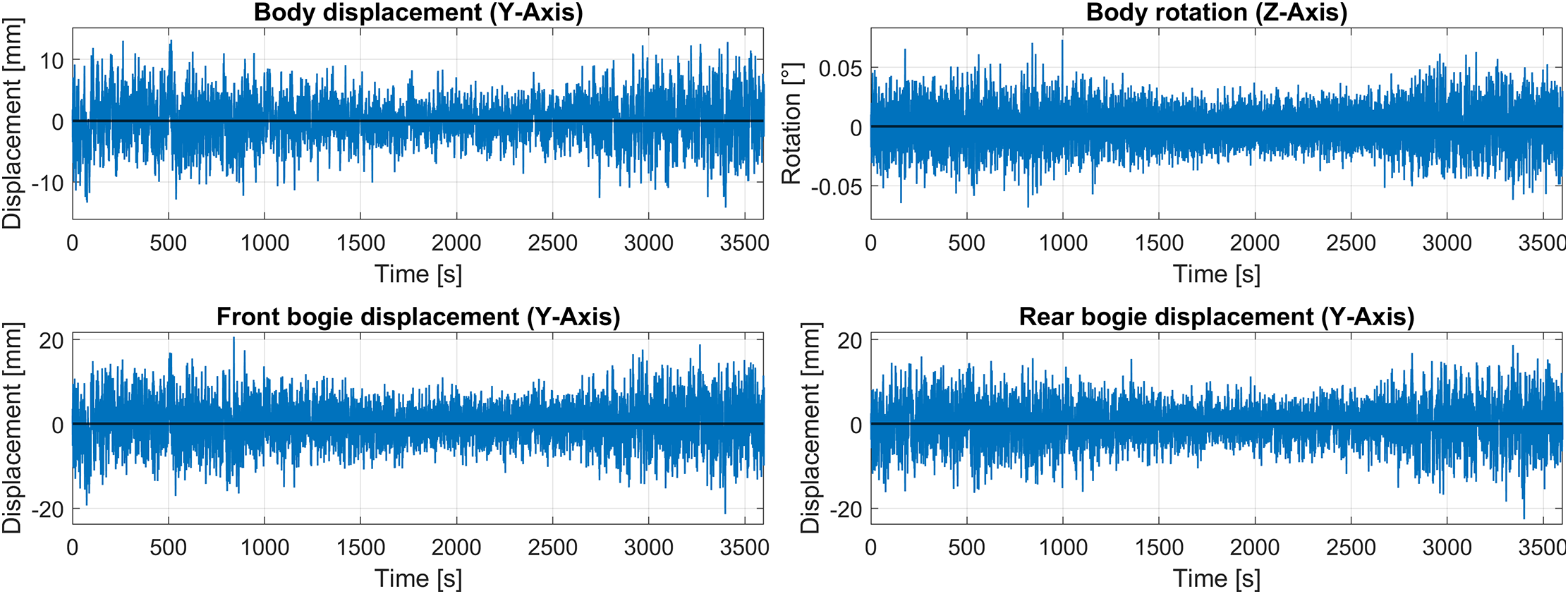
Figure 17: Response quantities for the Bouc-Wen model

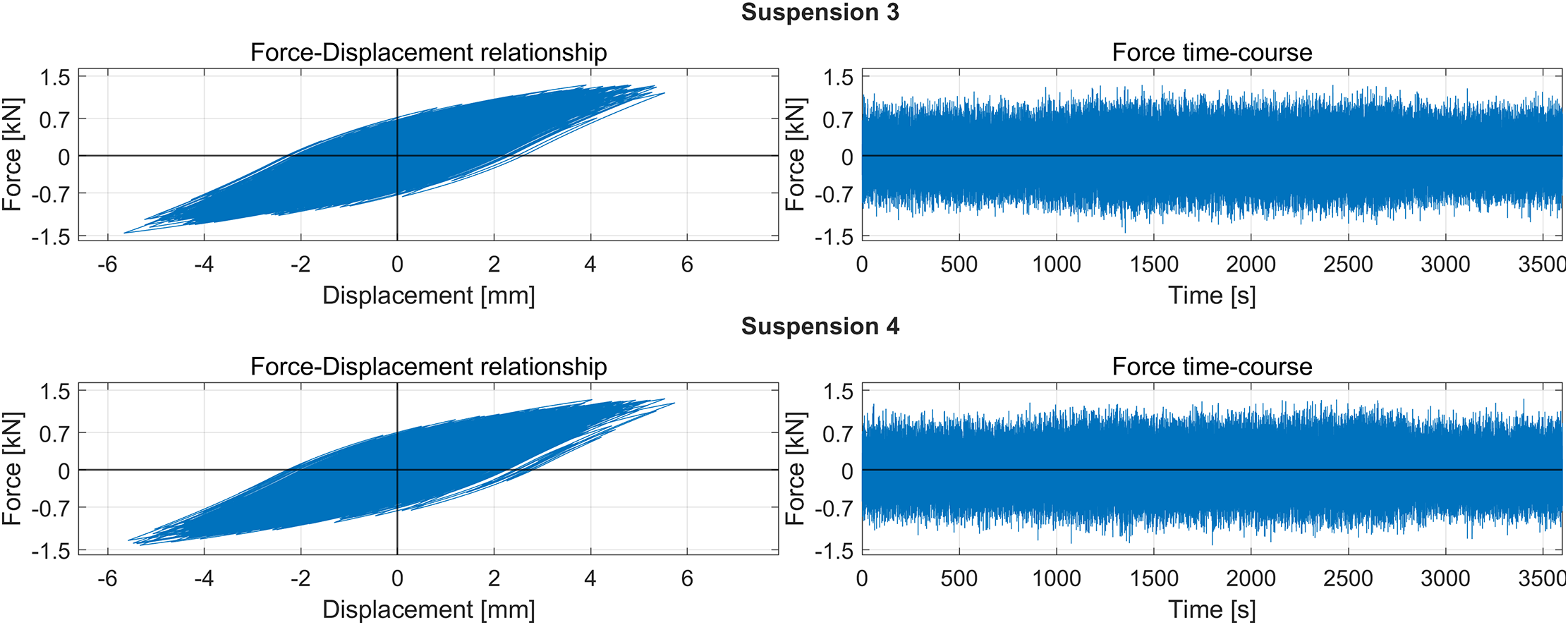
Figure 18: Hysteretic loops and force time courses for the Bouc-Wen model, suspension 3, 4

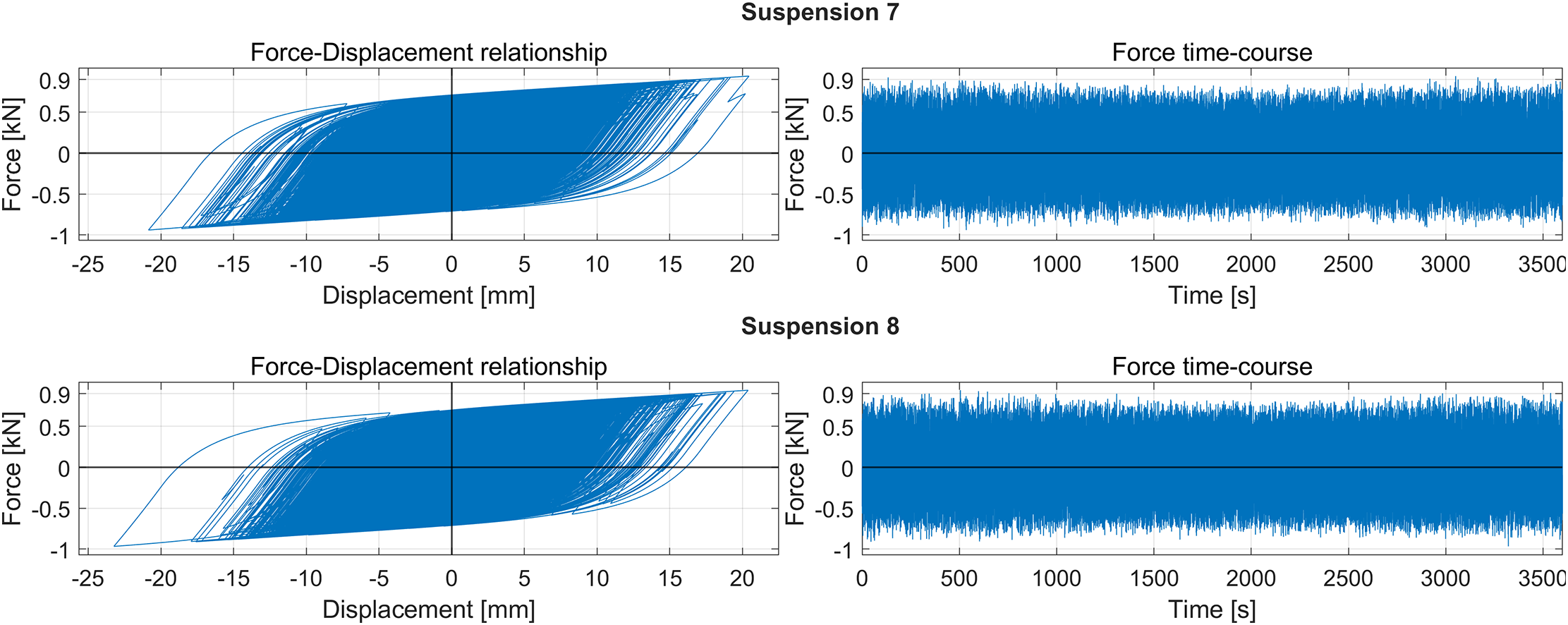
Figure 19: Hysteretic loops and force time courses for the Bouc-Wen model, suspension 7, 8.

4.4 Wang-Wen Model

The response quantities are shown in Fig. 20, and the hysteretic loops and forces are presented in Figs. 21 and 22. The asymmetric behaviour of the Wang-Wen model is reflected in the hysteresis loops as well as in the response quantities. Considering the loop shapes, the displacements are predominantly positive; thus, all the loops appear to be shifted to the right. Despite the asymmetric displacements, the maximum positive and negative forces have approximately the same value. This holds for all suspension components. As in the previous cases, the group B components exhibit larger displacements and thus their loops are wider, compared to group A.

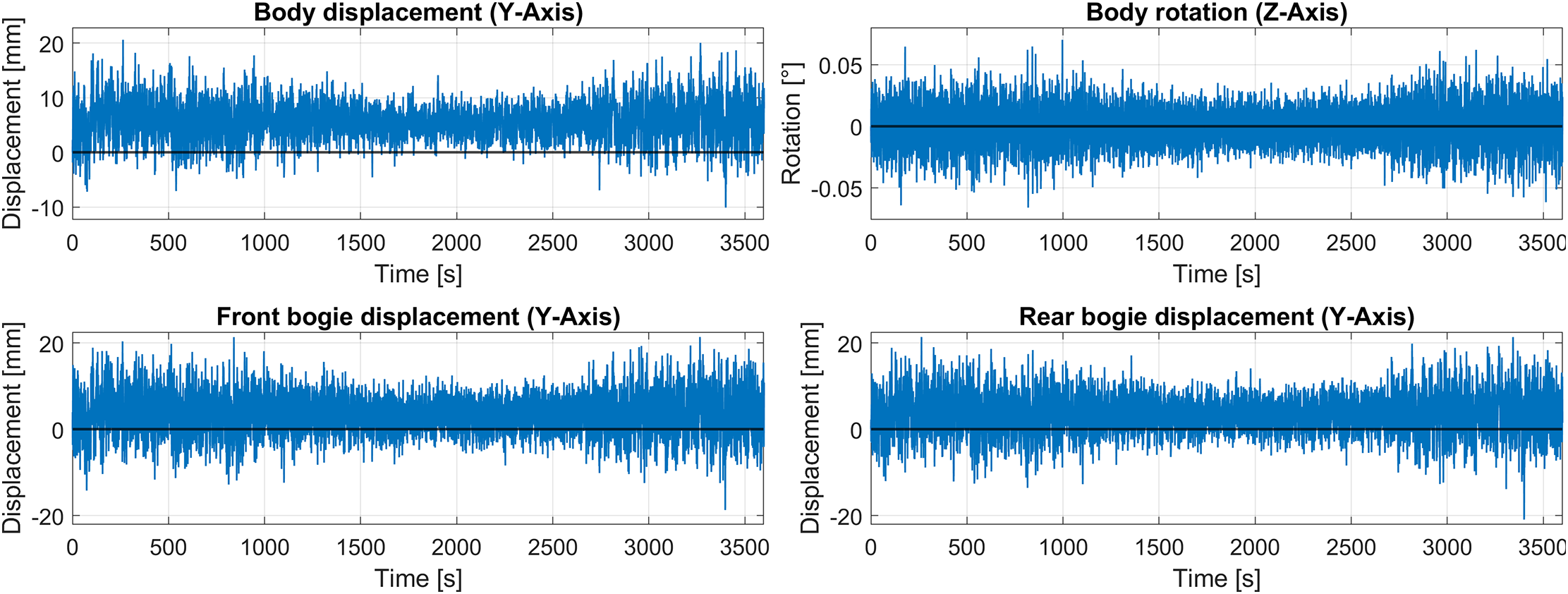
Figure 20: Response quantities for the Wang-Wen model

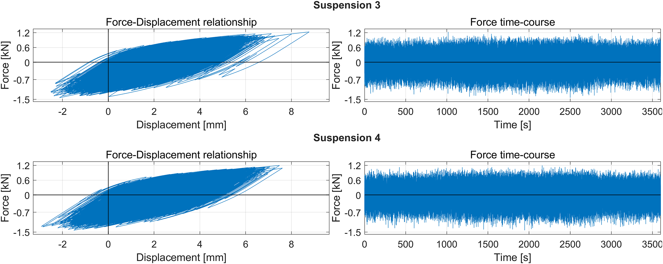
Figure 21: Hysteresis loops and force time courses for the Wang-Wen model, suspension 3, 4

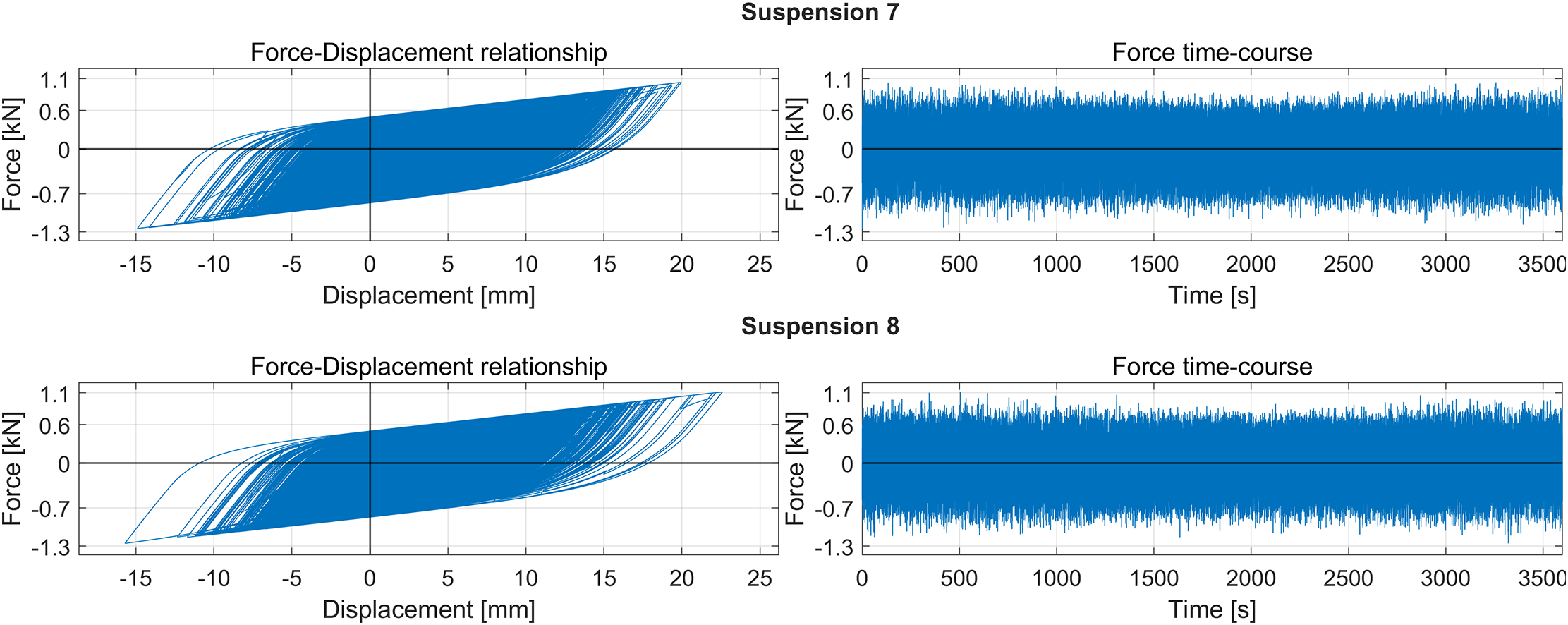
Figure 22: Hysteresis loops and force time courses for the Wang-Wen model, suspension 7, 8

4.5 Generalised Bouc-Wen Model

The time courses of the response quantities are shown in Fig. 23, and the hysteretic loops and forces are presented in Figs. 24 and 25. The asymmetric behaviour is again visible on the response quantities time courses as well as on the hysteresis loops, which possess a strongly asymmetric shape. As in the previous case, the displacements are predominantly positive for all suspension components and noticeably larger for group B components. Despite the asymmetric displacements, the maximum positive and negative forces are again approximately the same. This holds for both component groups.

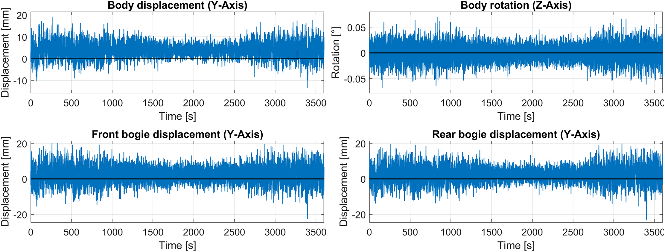
Figure 23: Response quantities for the generalised Bouc-Wen model

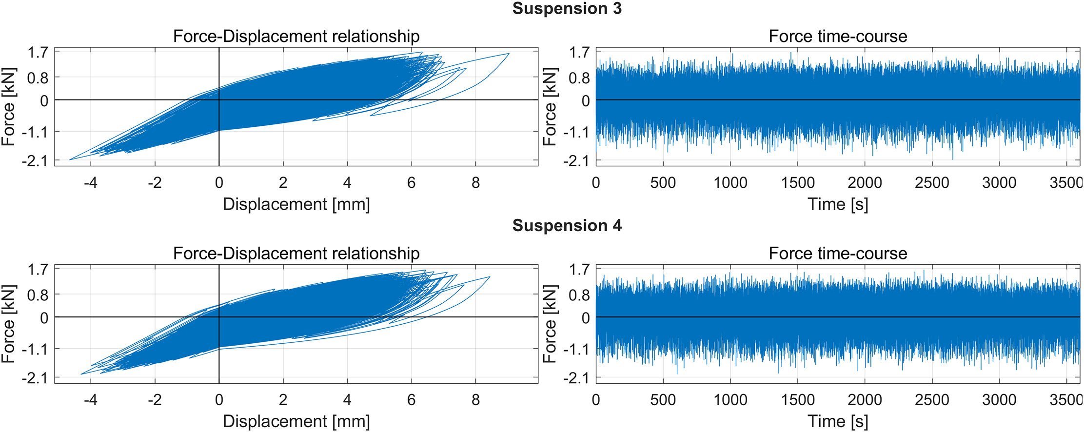
Figure 24: Hysteretic loops and respective force time courses for the generalised Bouc-Wen model, suspension 3, 4

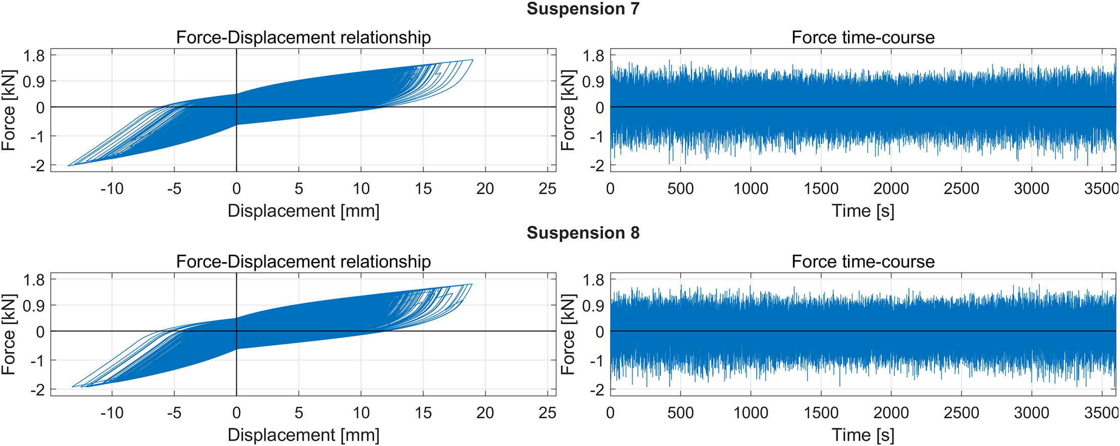
Figure 25: Hysteretic loops and respective force time courses for the generalised Bouc-Wen model, suspension 7, 8

5  Statistical Processing of the Results in the Time Domain

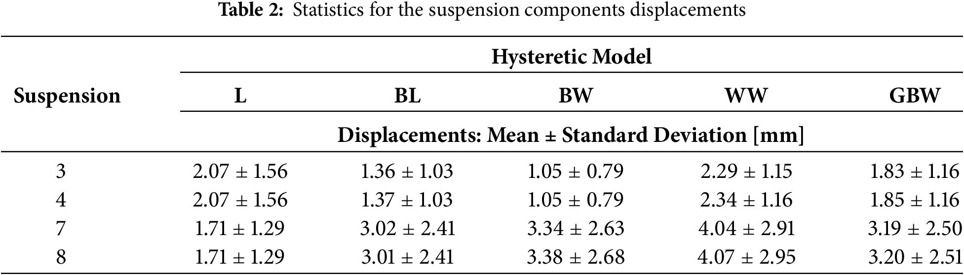
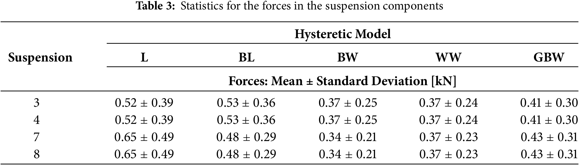
This section presents statistically processed results. Fig. 26 presents the statistics for the response quantities, with tabular data being presented in Table 1. Additionally, the statistics for the suspension components’ forces and displacements are presented in Figs. 27 and 28. The data in tabular form are displayed in Table 2, which shows the displacements, and Table 3 shows the hysteretic forces.

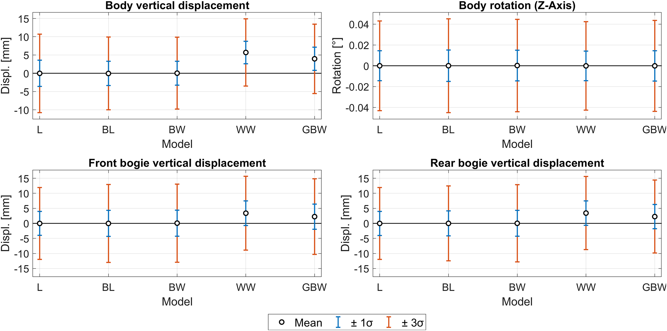
Figure 26: Statistical comparison of the response quantities

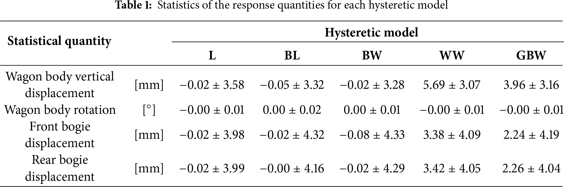
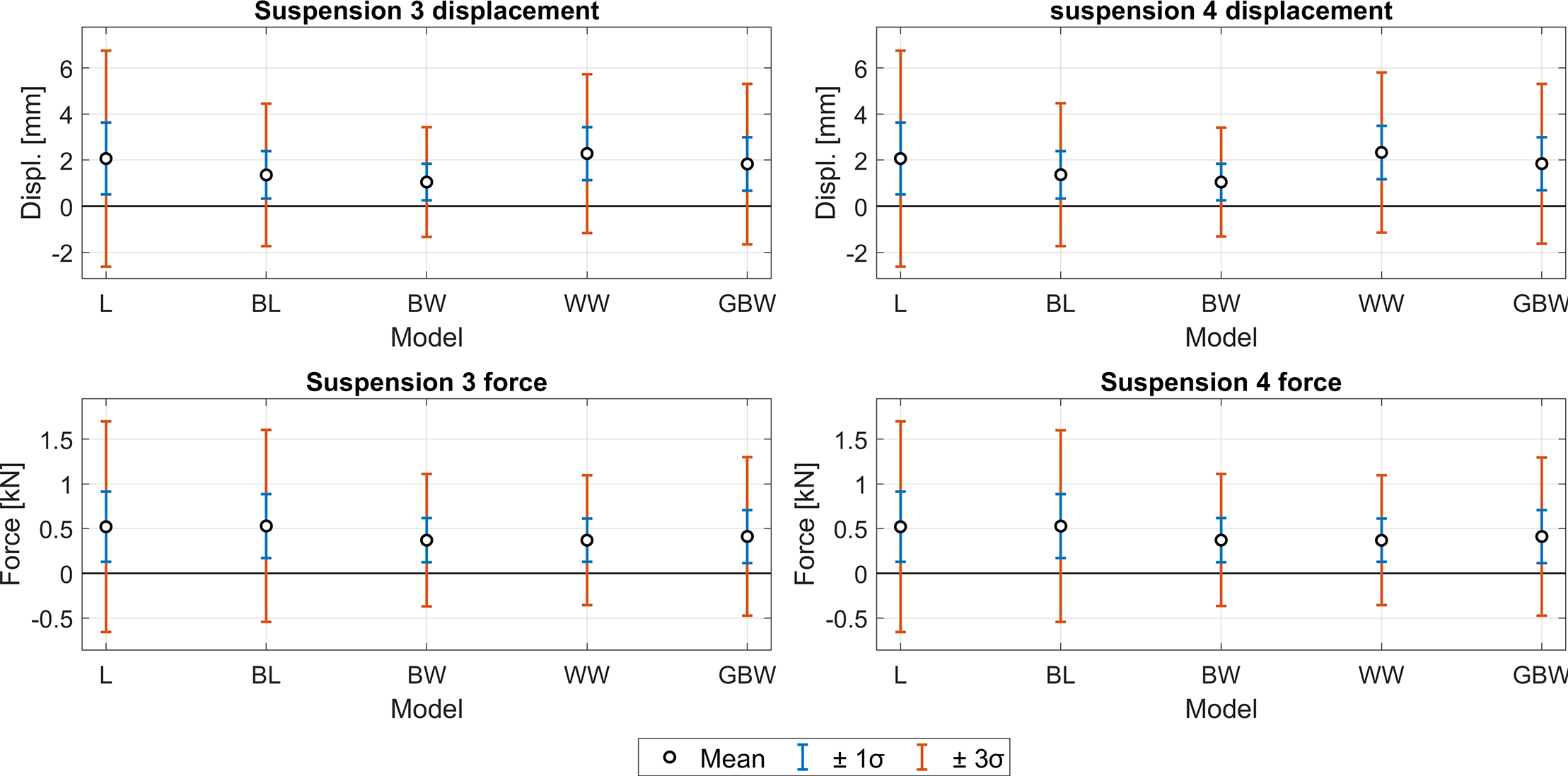
Figure 27: Statistics for the forces and displacements of the group A suspension components

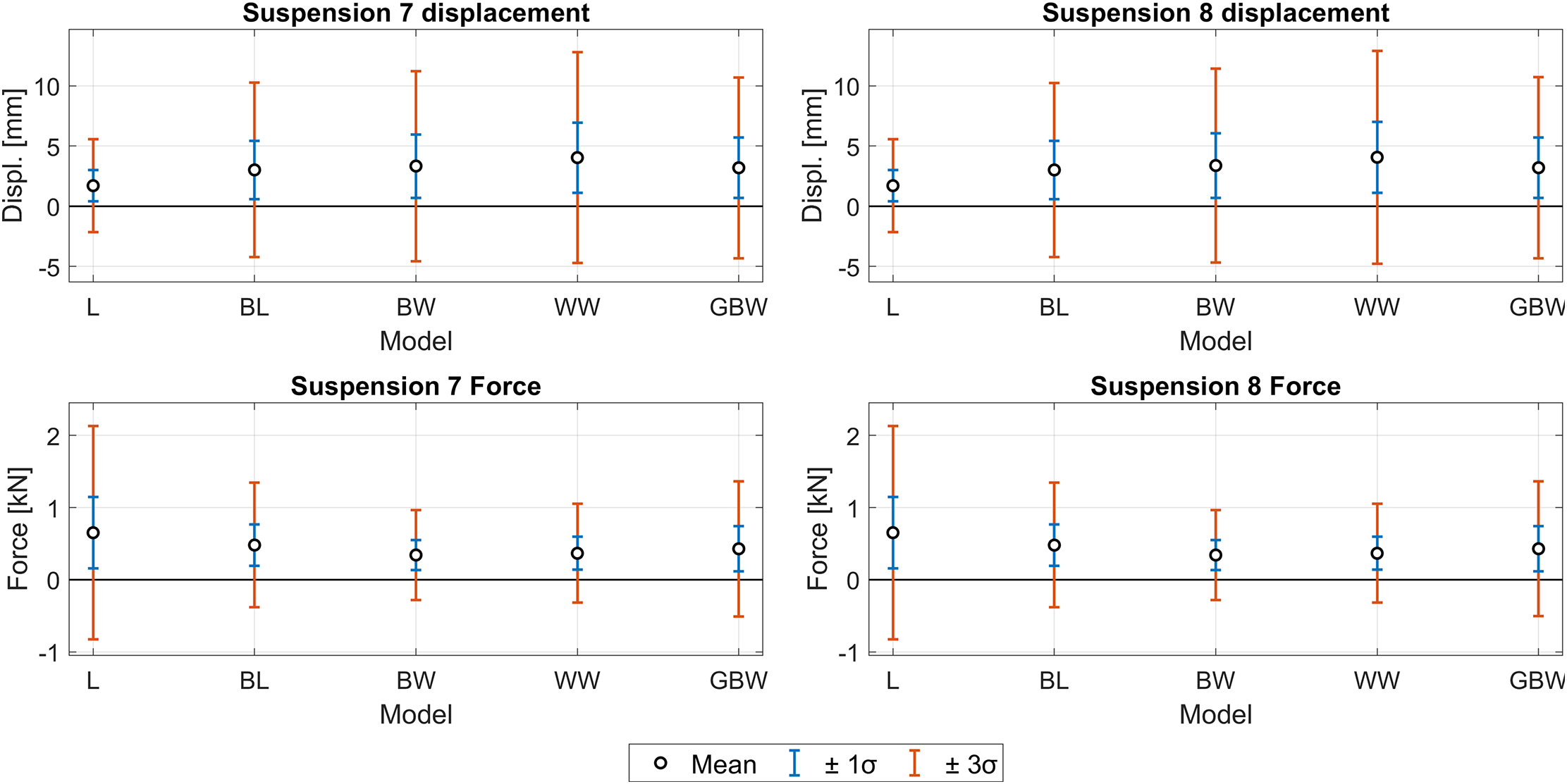
Figure 28: Statistics for the forces and displacements of the group B suspension components

In the case of the symmetric models, the results are statistically similar. There are only slight differences in mean values. However, the asymmetric behaviour of the Wang-Wen and generalised Bouc-Wen models is also reflected in the presented results. The mean values are shifted, which is more noticeable for the Wang-Wen model. The standard deviations are similar for all models; thus, they seem to be affected only minimally by the hysteresis. There are no noticeable differences in the data describing the body rotation, in both the mean values and the standard deviations. This might be attributed to the negligible displacements compared to the bogie distance. The data are additionally presented in Table 1.

The components of the suspension group A exhibit similar behaviour in terms of both the displacements and the forces. Considering the displacements, the mean values are nonzero for each model. These are the lowest for the Bouc-Wen and the bilinear model, which is true for their standard deviations as well. The mean values for asymmetric models are similar to the linear model; however, their standard deviations are lower.

The hysteretic forces are statistically similar to the linear model only in the case of the bilinear model. The other three models exhibit mutually comparable mean values as well as the standard deviations that are generally lower than in the case of linear and bilinear models. Considering the results, hysteresis affects the suspension behaviour regardless of the model used. Besides the shifts in mean values, the decrease in standard deviations can be observed.

Both components of the suspension group B again exhibit similar behaviour. Unlike in the case of the group A components, both the mean values and the standard deviations of the displacements are greater for the nonlinear hysteretic models. The largest values were achieved by the Wang-Wen model. Nevertheless, the hysteretic forces are affected in a similar way as in the previous case. Thus, the nonlinear models exhibit generally lower mean values and standard deviations than the linear model. Again, the hysteresis influences the suspension components, which is displayed by the changes in the examined statistical quantities. The presented results are additionally displayed in tabular form in Tables 2 and 3.

Considering the computational time, the simulated one-hour ride required approximately 20 to 30 min of computing. The calculations were performed on a standard desktop computer with an 11th Gen Intel Core i5-11400F @ 2.60 GHz CPU, with 32.0 GB DDR4 RAM. The least time-demanding was naturally the linear model. The bilinear and generalised Bouc-Wen models required the most time (roughly about 1.5 times more than other models). Despite the varying complexity of the formulations, all the hysteretic models require only one additional differential equation. The parameters of these models were calculated prior to the dynamic simulation. Therefore, the complexity of the models is not considered the main reason for the different computational times. The authors assume that the sharp stiffness changes play a significant role here. These are most evident in the bilinear model. Additional sharp edges occur in the generalised B-W model when there is a change in the displacement direction. These sharp changes in stiffness might be troublesome for the numerical solver, which requires more time to obtain a solution satisfying the required error tolerances.

6  Results Analysis in the Frequency Domain

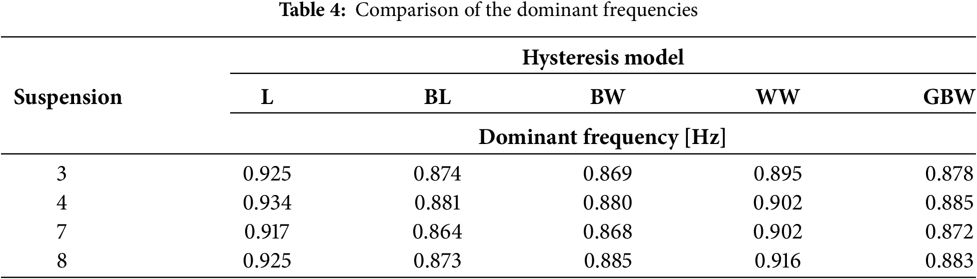
The following section presents the frequency analysis of the selected results in the form of power spectral densities (PSD). The results analysed were the vertical displacement of the car body, shown in Fig. 29, and the hysteretic forces in the front suspension displayed in Figs. 30 and 31. The dominant frequencies of the suspension forces are then compared in Fig. 32 and summarised in Table 4. All the PSDs were obtained with the use of the Welch’s approximation method available in MATLAB.

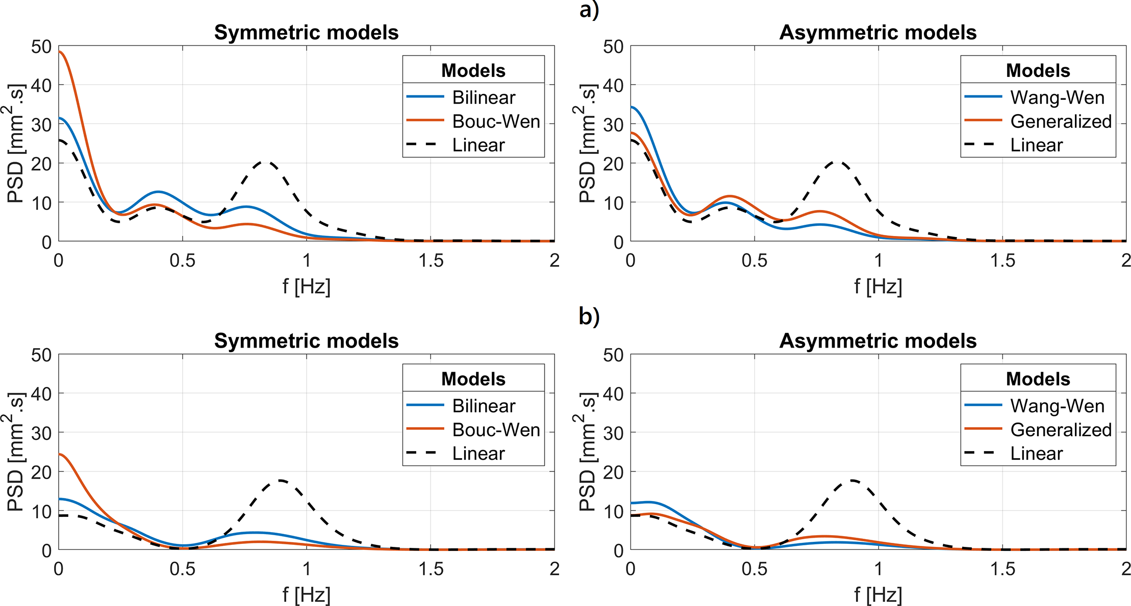
Figure 29: (a) PSDs of vertical body displacement for each hysteretic model; (b) The same results for the simulation with constant vehicle velocity

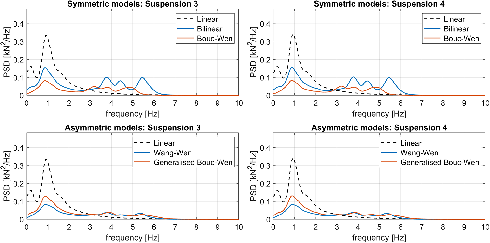
Figure 30: The PSDs of the forces in suspension components 3, 4

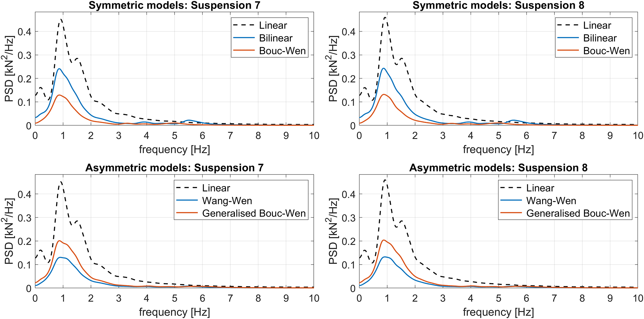
Figure 31: The PSDs of the forces in suspension components 7, 8

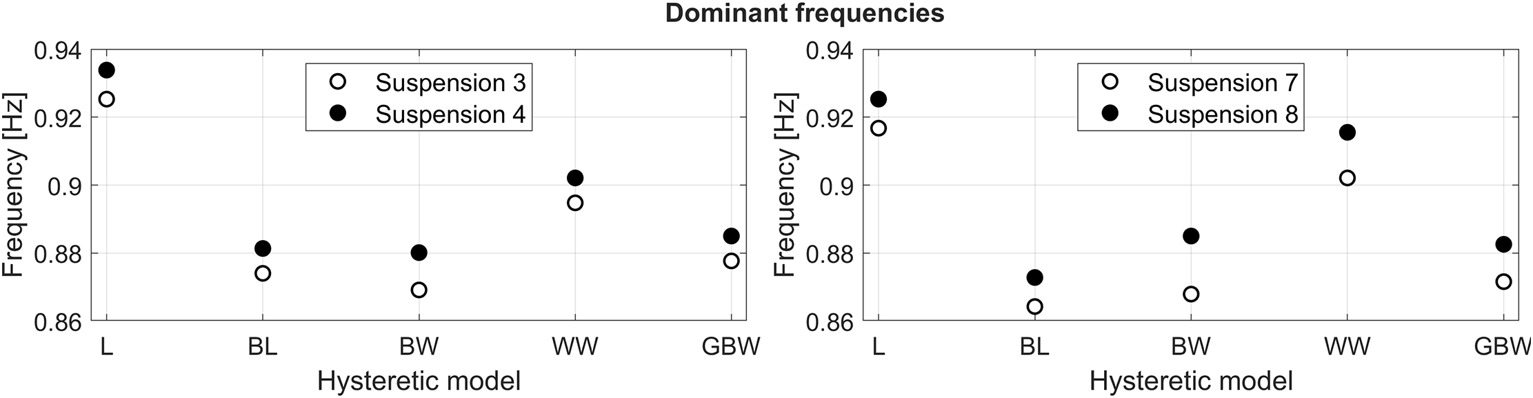
Figure 32: Comparison of the dominant frequencies in the suspension forces for each hysteretic model

The PSDs of the vertical body displacements (Fig. 29) were additionally smoothed to suppress the noise that was initially present in the results and to highlight the peaks corresponding to the dominant frequencies. For comparison, an additional simulation with a constant vehicle velocity of 25 m/s was performed. The corresponding PSDs are shown in the bottom part of Fig. 29.

There are 3 dominant frequencies present in the PSDs of the wagon body vertical displacement. These are represented by the peaks at approximately 0 Hz, 0.4 Hz and 0.7 Hz. The 0 Hz frequency corresponds to the shift in the mean value of the force. It can be observed in each hysteretic model; however, it is most dominant for the Bouc-Wen model. Considering the nonlinear models, the other two frequencies are significantly less distinct, with the highest frequency having the lowest peak. This is unlike the linear model, where the highest frequency is almost as dominant as the 0 Hz frequency. Additionally, it can be observed that the nonlinear models have slightly lower frequencies compared to the linear models.

In the case of constant vehicle velocity. There are only two dominant frequencies present, approximately 0.1 Hz and 0.8 Hz. The 0.4 Hz frequency is not present here. The shift of the peak at the 0 Hz frequency suggests the mean value of the force is less shifted. Similarly to the previous case, the peaks at 0.8 Hz are most distinct for the linear model. Considering the results, the hysteresis seems to suppress the higher frequencies while the lower ones become slightly more dominant. Additionally, the peaks in the PSDs appear at slightly lower frequencies.

The frequency spectra of the hysteretic forces in suspension components were also analysed. There is a noticeable peak at about 1 Hz, for all models and for all suspension components. In the case of a linear model, two additional peaks, at approximately 0.2 Hz and 1.5 Hz, can be observed. These are less dominant or even completely absent in the PSDs of nonlinear models. The peaks are generally lower for nonlinear models. Specifically, in the case of group A components, there are additional peaks in the range of 3 Hz to 6 Hz. The peaks are only present in nonlinear models and are most distinct in the bilinear model.

The cause of these peaks, as well as their physical meaning, is not completely clear for now. The authors assume, this phenomenon might be caused by the sharp changes of stiffness caused by the hysteretic models. These changes are most evident in the bilinear model producing rectangular hysteresis loops, but occur generally in all nonlinear models when the loading direction changes. Additionally, the inaccuracy of a numerical solver or numerical noise, caused by the mentioned stiffness changes, might be considered as well.

As stated before, the data was additionally filtered to obtain distinct peaks in the PSDs. The frequencies at which the highest peaks occur were obtained for each suspension component and plotted in Fig. 32. However, due to the smoothing, the data are only indicative and should be treated with caution.

As shown in Fig. 32, the dominant frequencies of the nonlinear models are lower compared to the linear model. This holds for each suspension component. Thus, the hysteresis seems to lower the values of PSDs, as well as the dominant frequencies in the systems. The frequencies are, however, influenced only to a limited extent. The data are additionally summarised in the following table (Table 4).

7  Conclusion

This work dealt with the dynamic analysis of a rail vehicle equipped with suspension components possessing hysteretic properties. The study focused primarily on the vehicle vertical oscillation and how it is influenced by the hysteretic models. The vehicle behaviour was studied in both the time and the frequency domains. The treated vehicle was modelled, and the obtained results were processed in the MATLAB environment. In the first part of the study, several types of hysteretic models are presented. Namely, the bilinear, Bouc-Wen, and the asymmetric models, the Wang-Wen, and the generalised Bouc-Wen model. As a reference, a linear model was used as well. The parameters of the presented models were then calculated based on the energy dissipation per loading cycle. In the second part of the study, the hysteretic models were implemented into the vehicle suspension, and the simulations were performed. The vehicle was treated as a system of three solid bodies with a total of 7 DOF. It was moving along an uneven track with varying velocity. The track vertical irregularities were modelled using the Kanai-Tajimi differential filter and served as a kinematic excitation function. The studied results were primarily the wagon body vertical oscillations and the hysteretic forces in suspension components. These results were then further processed, using the PSD approximation, to analyse the vehicle behaviour in the frequency domain. Here, primarily the dominant frequencies occurring during the vehicle motion were studied.

Considering the results and the selected model parameters, the symmetric hysteretic models seem to have no significant impact on the wagon body vertical motion. This is supported by mostly negligible differences in the mean values and the corresponding standard deviations of the wagon body displacements for each symmetric model. The same holds for the bogie displacements as well. However, in the case of asymmetric models, there is a noticeable increase in the mean values of the displacements. This suggests the asymmetric hysteretic behaviour is reflected in the vehicle motion. Thus, the wagon body, as well as the bogies, oscillate about shifted equilibrium positions.

Additionally, the forces and displacements of the front suspension components were analysed. The components were divided into two groups, each modelled using different parameter values. In the case of first group components, the hysteretic models generally showed lower standard deviations of displacements compared to the linear model. Moreover, the symmetric models resulted in lower mean values as well. In terms of forces, the hysteretic models show generally lower mean values and standard deviations. This is except for the bilinear model, which behaved relatively close to the linear model. The presented results suggest that the hysteresis causes more stable behaviour as a result of increased damping introduced to the system. Additionally, the asymmetric behaviour can be observed in the displacements, as a likely result of asymmetric hysteretic models.

The suspension components of the second group showed different behaviour, since their different parameter values and different bodies they are connecting. Generally, the increase in displacements, manifested by greater standard deviations, together with shifted mean values, can be observed in hysteretic models. On the contrary, the restoring forces are noticeably lower compared to the linear model. This is mostly visible in the presented standard deviations of the forces. This behaviour implies lower stiffness of hysteretic components, with no significant differences between symmetric and asymmetric models. Thus, there is a distinct difference in the behaviour of each component group.

The presented results were then processed to obtain the corresponding PSDs, showing dominant frequencies occurring in the system. The frequencies at which the wagon body oscillates and the frequencies of restoring forces in the front bogie suspension were analysed. In the case of the body motion, there is no noticeable change in frequencies caused by the hysteresis. However, the hysteresis seems to suppress the PSDs of higher frequencies and slightly increase them for the lower frequencies. This is noticeable mostly in the Bouc-Wen model. Considering the suspension forces, the results are similar to those in the previous case. The hysteretic models showed only slightly decreased dominant frequencies; however, with noticeably reduced PSDs. This is common for all hysteretic models, whether they are symmetric or asymmetric. Again, the behaviour of the hysteretic system implies increased energy dissipation in the suspension components, compared to the linear model.

Considering the computing time, the models producing sharp stiffness changes are generally more computationally expensive. The sharp stiffness changes are produced by all nonlinear models when the loading direction changes. However, in the case of bilinear and generalised B-W models, this phenomenon occurs more often. This is considered to be the main reason these models require approximately 1.5 times more computing time. Nevertheless, for the simulated one-hour ride, the total calculation time ranged from 20 to 30 min. Therefore, the presented models might be suitable for real-time analyses. However, the model complexity and the utilised hardware need to be considered.

The presented results show that the hysteresis influences both the motion and the frequency response of the treated vehicle model. Each hysteretic model has its own characteristics that impact the system behaviour. This is also reflected in the system’s natural frequencies, which represent important characteristics of each mechanical system. Considering the presented results, the asymmetric hysteretic models show generally greater impact on the system behaviour, compared to the symmetric models. Additionally, these models offer greater flexibility regarding the hysteretic loop shapes. Generally, all the presented hysteretic models can be utilised in the modelling of the damaged components. However, due to their greater flexibility, the asymmetric models, and mainly the generalised Bouc-Wen, can be potentially considered as the most suitable. This is despite the increased computing time.

At the current stage of the study, the main objective is the implementation of hysteresis models into mechanical systems and the suitability research of these models, in the context of diagnostics and digital twin modelling. The practical implementation of the presented concept has not been fully developed yet. Therefore, this study, at its current state, only suggests the possible applications, which will be the subjects of further research and represent the main limitations of this work.

Acknowledgement: The authors would like to thank Dr. Daniela Sršníková for her help with the translation of this article.

Funding Statement: This work was supported by projects KEGA, Nos. 002ŽU-4/2023, and 005ŽU-4/2024, and by the project VEGA, No. 1/0423/23.

Author Contributions: The authors confirm contribution to the paper as follows: Conceptualisation, Milan Sága; methodology, Milan Sága; software, Ján Minárik; formal analysis, Ján Minárik; resources, Milan Sága, Milan Vaško; data curation, Ján Minárik; writing—original draft preparation, Ján Minárik; writing—review and editing, Milan Vaško, Jaroslav Majko; visualisation, Jaroslav Majko; supervision, Milan Sága, Milan Vaško; funding acquisition, Milan Sága, Milan Vaško. All authors reviewed and approved the final version of the manuscript.

Availability of Data and Materials: The data that support the findings of this study are available from the Corresponding Author, [Ján Minárik], upon reasonable request.

Ethics Approval: Not applicable.

Conflicts of Interest: The authors declare no conflicts of interest.

References

1. Zhong D, Xia Z, Zhu Y, Duan J. Overview of predictive maintenance based on digital twin technology. Heliyon. 2023;9(4):e14534. doi:10.1016/j.heliyon.2023.e14534. [Google Scholar] [PubMed] [CrossRef]

2. Wu J, Yang Y, Cheng X, Zuo H, Cheng Z. The development of digital twin technology review. In: Proceedings of the 2020 Chinese Automation Congress (CAC); 2020 Nov 6–8; Shanghai, China. doi:10.1109/cac51589.2020.9327756. [Google Scholar] [CrossRef]

3. Song J, Der Kiureghian A. Generalized Bouc-Wen model for highly asymmetric hysteresis. J Eng Mech. 2006;132(6):610–8. doi:10.1061/(asce)0733-9399(2006)132:. [Google Scholar] [CrossRef]

4. Wang T, Noori M, Altabey WA, Wu Z, Ghiasi R, Kuok SC, et al. From model-driven to data-driven: a review of hysteresis modeling in structural and mechanical systems. Mech Syst Signal Process. 2023;204:110785. doi:10.1016/j.ymssp.2023.110785. [Google Scholar] [CrossRef]

5. Wu Z, Liu B, Wei J, Yang Y, Zhang X, Deng J. Design of porous shape memory alloys with small mechanical hysteresis. Crystals. 2023;13(1):34. doi:10.3390/cryst13010034. [Google Scholar] [CrossRef]

6. Ismail M, Ikhouane F, Rodellar J. The hysteresis Bouc-Wen model, a survey. Arch Comput Meth Eng. 2009;16(2):161–88. doi:10.1007/s11831-009-9031-8. [Google Scholar] [CrossRef]

7. Zhu X, Lu X. Parametric identification of Bouc-Wen model and its application in mild steel damper modeling. Procedia Eng. 2011;14:318–24. doi:10.1016/j.proeng.2011.07.039. [Google Scholar] [CrossRef]

8. Halama R, Fusek M, Poruba Z. Influence of mean stress and stress amplitude on uniaxial and biaxial ratcheting of ST52 steel and its prediction by the AbdelKarim-Ohno model. Int J Fatigue. 2016;91:313–21. doi:10.1016/j.ijfatigue.2016.04.033. [Google Scholar] [CrossRef]

9. Bartošák M, Horváth J, Španiel M. Multiaxial low-cycle thermo-mechanical fatigue of a low-alloy martensitic steel: cyclic mechanical behaviour, damage mechanisms and life prediction. Int J Fatigue. 2021;151:106383. doi:10.1016/j.ijfatigue.2021.106383. [Google Scholar] [CrossRef]

10. Wang W, Zhang W, Wang E. Generation and modeling of asymmetric hysteresis damping characteristics for a symmetric magnetorheological damper. In: Proceedings of the 2009 Second International Conference on Intelligent Computation Technology and Automation; 2009 Oct 10–11; Changsha, China. doi:10.1109/icicta.2009.511. [Google Scholar] [CrossRef]

11. Zhou J, Wen C. Adaptive feedback control of magnetic suspension system preceded by Bouc-Wen hysteresis. In: Proceedings of the 2012 12th International Conference on Control Automation Robotics & Vision (ICARCV); 2012 Dec 5–7; Guangzhou, China. p. 1244–9. doi:10.1109/icarcv.2012.6485323. [Google Scholar] [CrossRef]

12. Eizmendi M, Heras I, Aguirrebeitia J, Abasolo M. Hysteretic damping model for the dynamic response in four-point contact slewing bearings. Mech Mach Theory. 2025;214:106150. doi:10.1016/j.mechmachtheory.2025.106150. [Google Scholar] [CrossRef]

13. Wu Z, Xiang Y, Liu C. Influence of suspension hysteresis characteristics on vehicle vibration performance. Proc Inst Mech Eng Part D J Automob Eng. 2021;235(5):1211–24. doi:10.1177/0954407020970839. [Google Scholar] [CrossRef]

14. Rathore KK, Singh AP, Kanchwala H, Biswas S. A comprehensive experimental and numerical study of hysteretic characteristics of leaf spring suspensions. J Vib Eng Technol. 2025;13(5):264. doi:10.1007/s42417-025-01825-6. [Google Scholar] [CrossRef]

15. Klockiewicz Z, Ślaski G. The influence of friction force and hysteresis on the dynamic responses of passive quarter-car suspension with linear and non-linear damper static characteristics. Acta Mech Autom. 2023;17(2):205–18. doi:10.2478/ama-2023-0024. [Google Scholar] [CrossRef]

16. Moradi Nerbin M, Mojed Gharamaleki R, Mirzaei M. Novel optimal control of semi-active suspension considering a hysteresis model for MR damper. Trans Inst Meas Control. 2017;39(5):698–705. doi:10.1177/0142331215618446. [Google Scholar] [CrossRef]

17. Jönsson PA, Andersson E, Stichel S. Influence of link suspension characteristics variation on two-axle freight wagon dynamics. Veh Syst Dyn. 2006;44(1):415–23. doi:10.1080/00423110600872416. [Google Scholar] [CrossRef]

18. Zambare H, Khoje A, Patil S, Razban A. MR damper modeling performance comparison including hysteresis and damper optimization. IEEE Access. 2021;9:24560–9. doi:10.1109/access.2021.3057174. [Google Scholar] [CrossRef]

19. Dai D, Zhang J, Zhang B, Li P, Hu W. Adaptive hierarchical optimization control for electrohydraulic suspension with resistor-capacitor operator. Appl Math Model. 2024;126:606–24. doi:10.1016/j.apm.2023.11.018. [Google Scholar] [CrossRef]

20. Jayaraman T, Thangaraj M. Standalone and interconnected analysis of an independent accumulator pressure compressibility hydro-pneumatic suspension for the four-axle heavy truck. Actuators. 2023;12(9):347. doi:10.3390/act12090347. [Google Scholar] [CrossRef]

21. Deng M, Kin Wong P, Gao Z, Ma X, Zhao J. Robust finite frequency control for MRF damper-based semi-active suspension systems subject to time delay and hysteresis nonlinearity. Proc Inst Mech Eng Part I J Syst Control Eng. 2025;239(1):151–72. doi:10.1177/09596518241262502. [Google Scholar] [CrossRef]

22. Klockiewicz Z, Ślaski G. Comparison of vehicle suspension dynamic responses for simplified and advanced adjustable damper models with friction, hysteresis and actuation delay for different comfort-oriented control strategies. Acta Mech Autom. 2023;17(1):1–15. doi:10.2478/ama-2023-0001. [Google Scholar] [CrossRef]

23. Kalmár-Nagy T, Shekhawat A. Nonlinear dynamics of oscillators with bilinear hysteresis and sinusoidal excitation. Phys D Nonlinear Phenom. 2009;238(17):1768–86. doi:10.1016/j.physd.2009.06.016. [Google Scholar] [CrossRef]

24. Hua CR, Zhao Y, Lu ZW, Ouyang H. Random vibration of vehicle with hysteretic nonlinear suspension under road roughness excitation. Adv Mech Eng. 2018;10:1–10. doi:10.1177/1687814017751222. [Google Scholar] [CrossRef]

25. Hu R, Zhang D, Deng Z, Xu C. Stochastic analysis of a nonlinear energy harvester with fractional derivative damping. Nonlinear Dyn. 2022;108(3):1973–86. doi:10.1007/s11071-022-07338-1. [Google Scholar] [CrossRef]

26. Hu R, Lu K, Zeng Z, Zhou S, Xie Z, Deng Z. Nonlinear dynamic analysis of the vibration energy harvester with hysteresis characteristics under random excitations. Int J Non Linear Mech. 2025;178:105216. doi:10.1016/j.ijnonlinmec.2025.105216. [Google Scholar] [CrossRef]

27. Yuan Z, Chen L, Sun JQ. Stochastic dynamics of hysteresis systems under harmonic and Poisson excitations. Chaos Solitons Fractals. 2025;198:116540. doi:10.1016/j.chaos.2025.116540. [Google Scholar] [CrossRef]

28. Vaiana N, Sessa S, Rosati L. A generalized class of uniaxial rate-independent models for simulating asymmetric mechanical hysteresis phenomena. Mech Syst Signal Process. 2021;146:106984. doi:10.1016/j.ymssp.2020.106984. [Google Scholar] [CrossRef]

29. Dumitriu M. Method to synthesize the track vertical irregularities. Sci Bull Petru Maior Univ Tîrgu Mureş. 2014;11(2):17–24. doi:10.2478/rjti-2018-0011. [Google Scholar] [CrossRef]

30. Saga M. Contribution to the analysis of non-stationary random vibration of vehicles. Commun Sci Lett Univ Žilina. 2001;3(1):35–43. doi:10.26552/com.c.2001.1.35-43. [Google Scholar] [CrossRef]