
 Submit a Paper
 Propose a Special lssue
 Open Access
ARTICLE

Explainable Ensemble Learning Approach for Ovarian Cancer Diagnosis Using Clinical Data
1 Skolkovo Institute of Science and Technology (Skoltech), Moscow, Russia
2 Department of Mathematics and Statistics, College of Science, Imam Mohammad Ibn Saud Islamic University (IMSIU), Riyadh, Saudi Arabia
3 Department of Mathematics and Sciences, College of Sciences and Humanities, Prince Sultan University, Riyadh, Saudi Arabia
4 Department of Mathematics, COMSATS University Islamabad, Park Road, Islamabad, Pakistan
* Corresponding Author: Daniyal Asif. Email:
(This article belongs to the Special Issue: Artificial Intelligence Models in Healthcare: Challenges, Methods, and Applications)
Computer Modeling in Engineering & Sciences 2026, 146(3), 38 https://doi.org/10.32604/cmes.2026.077334
Received 07 December 2025; Accepted 02 March 2026; Issue published 30 March 2026
 View Full Text
 Download PDF
Abstract
Ovarian cancer (OC) is one of the leading causes of death related to gynecological cancer, with the main difficulty of its early diagnosis and a heterogeneous nature of tumor biomarkers. Machine learning (ML) has the potential to process complex datasets and support decision-making in OC diagnosis. Nevertheless, traditional ML models tend to be biased, overfitting, noisy, and less generalized. Moreover, their black-box nature reduces interpretability and limits their practical clinical applicability. In this study, we introduce an explainable ensemble learning (EL) model, TreeX-Stack, based on a stacking architecture that employs tree-based learners such as Decision Tree (DT), Random Forest (RF), Gradient Boosting (GB), and Extreme Gradient Boosting (XGBoost) as base learners, and Logistic Regression (LR) as the meta-learner to enhance ovarian cancer (OC) diagnosis. Local Interpretable Model-Agnostic Explanations (LIME) are used to explain individual predictions, making the model outputs more clinically interpretable and applicable. The model is trained on the dataset that includes demographic information, blood test, general chemistry, and tumor markers. Extensive preprocessing includes handling missing data using iterative imputation with Bayesian Ridge and addressing multicollinearity by removing features with correlation coefficients above 0.7. Relevant features are then selected using the Boruta feature selection method. To obtain robust and unbiased performance estimates during hyperparameter tuning, nested cross-validation (CV) with grid search is employed, and all experiments are repeated five times to ensure statistical reliability. TreeX-Stack demonstrates excellent diagnostic performance, achieving an accuracy of 0.9027, a precision of 0.8673, a recall of 0.9391, and an F1-score of 0.9012. Feature-importance analyses using LIME and permutation importance highlight Human Epididymis Protein 4 (HE4) as the most significant biomarker for OC. The combination of high predictive performance and interpretability makes TreeX-Stack a reliable tool for clinical decision support in OC diagnosis.Keywords
OC is one of the most deadly gynecological cancers that causes a large number of cancer deaths in women around the world. The World Health Organization recently estimated that OC causes more than 300,000 new cases and 200,000 deaths each year. This makes it the eighth most frequent disease among women worldwide [1]. OC is commonly diagnosed late because it doesn’t show any symptoms in its early stages, and there aren’t any accurate screening tests available. This greatly lowers the survival rate. The five-year survival rate is over 90% when the disease is found early, but it dips below 30% when it is more advanced [2]. So, it is very important to make sure that diagnostic systems are accurate and up-to-date in order to improve patient outcomes.
OC happens when cells in the ovaries expand and divide in an uncontrolled way [3]. People often call it a “silent killer” because it usually grows and spreads without any obvious signs in the beginning stages [4]. The disease is usually difficult to detect early, as symptoms typically appear when it is already advanced. The known risk factors of OC include older age, a history of the disease in the family, being overweight, and never having been pregnant or having children later in life, and endometriosis are all common risk factors of OC [5–7].
Despite extensive research, professionals have not yet developed a reliable approach to early diagnosis of OC, which remains one of the most substantial challenges in the management of the illness to date [8]. When health workers believe that a person might have OC, they would commonly begin by examining the patient, focusing on the symptoms, as well as performing a pelvic examination of the person to determine whether there are issues with the reproductive organs, including the vagina, uterus, ovaries, Fallopian tubes, and the cervix. It is recommended that the results be further tested. These can include imaging techniques such as Magnetic Resonance Imaging and Positron Emission Tomography, which help visualize internal structures to determine the presence of tumors [9,10]. Blood tests, particularly those that are to detect tumour markers, are also prevalent. The most famous of them is CA-125. The presence of high levels of CA-125 is indicative of OC. Not all patients, particularly during the initial phases, demonstrate an increase in CA-125 levels, which limits its use as a diagnostic marker. CA-125, in its turn, is frequently combined with other types of diagnoses to enhance the precision of the results [11]. There are instances in which OC cannot be reliably detected until after surgery, when it is tested on tissue, and the results indicate malignancy [12].
The diagnostic procedures are clinically practical but tedious, require expert medical knowledge, and rely on manual interpretation of findings. This manual process is time-consuming compared with automated approaches for diagnosing the disease [13]. In this way, even among experienced practitioners, subtle signs may be missed; therefore, data-driven techniques for early and accurate diagnosis are required. ML has already become an indispensable component of the medical domain, given the vast volumes of medical information available today [14,15]. ML can help uncover hidden patterns in complex medical data, predict outcomes, and inform decisions that benefit clinicians. In this case, the time to diagnosis is decreased, and ML has enhanced the accuracy of prediction, which helps in cancer diagnosis and can be improved in the future [16]. Nevertheless, there are practical constraints: without proper validation, ML models may not generalize well. This limitation can be mitigated by using robust and well-tested models [17]. Single models are prone to error, whereas ensembles, which combine multiple models, can yield more accurate and robust forecasts. EL combines the results of different models to enhance overall performance and minimize the risk of misclassification [18]. Another weakness is that most ML models are black boxes. They fail to provide explanations for their predictions, which is important in clinical practice, where it is important to understand why a model makes the choices it does [19,20].
To address these issues, this paper introduces TreeX-Stack, an explainable EL model for OC diagnosis. The tree-based learners that were incorporated into the model are DT, RF, XGBoost, and GB. LR is a meta-classifier that improves the predictions of base models. Several preprocessing steps are applied to ensure high data quality. Iterative imputation with Bayesian Ridge is used to handle missing values in the dataset. To address multicollinearity, features with correlation coefficients greater than 0.7 were excluded. The most relevant diagnostic features were then identified using the Boruta feature selection method. The interpretability of the model is further enhanced by LIME, which analyzes individual predictions and identifies the features with the greatest influence on its decisions. The proposed TreeX-Stack framework is a promising solution for an intelligent, interpretable, and clinically adaptable OC diagnosis system.
The remainder of the paper is as follows: Section 2 presents a literature review that summarizes recent research findings and discusses their limitations. This section also discusses the novelty of the current study and how it addresses gaps in the literature. In Section 3, the data used, data features, data preparation steps, the proposed model, and evaluation methods are discussed. The results are presented in Section 4 and include an explainability analysis, and an ablation study. Section 5 will provide a detailed discussion and compare the proposed model and identified biomarkers with the findings of previous studies. Lastly, Section 6 concludes the study and discusses the potential future research directions.
OC is among the most common types of cancer among women in the world. It can be diagnosed through clinical examination, which involves review of the medical history, assessment of symptoms, and physical examination [21,22]. The disease is traditionally detected and graded using positron emission tomography, computed tomography, and magnetic resonance imaging [23,24]. The diagnostic process also includes laboratory and pathological examinations, such as routine blood tests, comprehensive biochemical testing, and tumor marker analysis [25,26]. As medical data keeps growing, the application of ML in healthcare has expanded significantly. ML can analyze complex datasets, uncover hidden patterns, and enhance cancer detection [27–29]. These methods have, in recent years, been increasingly used to detect OC and to distinguish between benign and malignant tumours [30,31].
The data used in this study are available publicly and have been widely used in previous studies. It contains 49 characteristics, including demographic information, blood test, general chemistry test, and tumour markers. This dataset consist of records of 349 individuals, 171 of whom had OC and 178 had benign ovarian tumours. The pathological diagnosis of all patients was checked after surgery. None of the patients with OC had chemotherapy or radiation therapy before surgery. The patients’ ages range from 15 to 83 years. The dataset can be found on the Mendeley Data repository [32]. This literature review analyses current research employing the same dataset, emphasizing their techniques, principal findings, strengths, and limitations.
In 2025, multiple papers presented ML models utilizing the same OC dataset. Dhingra and Shetty [33] used median imputation to impute missing values and a Z-score to eliminate outliers. Z-score standardization and Principal Component Analysis (PCA) reduced the dimensionality of the dataset. They identified important features using Recursive Feature Elimination (RFE), Univariate Feature Selection, a correlation-based version, and an Autoencoder-based feature extraction. The models tested included K-Nearest Neighbors (KNN), Support Vector Machine (SVM), LR, and RF. EL techniques, including stacking, bagging, and boosting, were also explored. Various deep learning (DL) models were evaluated, including Artificial Neural Networks (NN), Recurrent NN, Convolutional NN, and Feedforward NN. The feedforward NN, which uses the autoencoder to select features, achieved the best classification accuracy of 85.71%. Öznacar and Güler [34] use the Iterative Imputer to impute missing data and use different techniques of feature selection, such as PCA, Boruta, RFE, and Mutual Information. They experiment RF, XGBoost, CatBoost, DT, KNN, Naive Bayes (NB), GB and SVM classifiers. It was shown that CatBoost with Boruta feature selection achieved the highest accuracy of 89.52%. Even if the results were encouraging, these research faced several limitations, including potential data leakage from simple train-test splitting, multicollinearity among features, and a lack of explainable AI methods for clinical interpretation.
A lot of papers looked at ML methods for OC classification using the same dataset in 2024. Newaz et al. [35] utilized Multivariate Imputation by Chained Equations to address missing data and standardized the features employing the Z-score approach. A genetic approach was utilized for feature selection, and various biomarkers were examined for premenopausal and postmenopausal populations. They used 10-fold CV to see how well the model worked. The XGBoost model got 0.896 for the premenopausal group and 0.958 for the postmenopausal group. They also used Shapely Additive explanations (SHAP) to make the model easier to understand. Acosta-Jiménez et al. [36] conducted another study employing a genetic approach for feature selection and assessed various ML models, including SVM, RF, and LR. LR performed best with an AUC of 0.9055. Sheela Lavanya and Subbulakshmi [37] identified 18 key features using Minimum Redundancy Maximum Relevance for feature selection. They evaluated various ML and ensemble learning (EL) models, including SVM, Decision Tree (DT), KNN, as well as voting, stacking, bagging, and boosting ensembles. The best-performing model was the ensemble, achieving an accuracy of 89%. Model interpretability and the importance of key features were assessed using SHAP and permutation importance. In another study by Jamalpour et al. [38], hierarchical clustering identified patterns distinguishing benign from malignant tumours. They developed a classification model that achieved an accuracy of 89.4%. These studies contributed to the literature, but they had some drawbacks, such as data leakage from simple data splitting instead of CV, limited explainability in some models, poor model evaluation methods, and a reliance on single models instead of EL methods, which are better for medical applications.
In previous years, other studies classified OC tumors using the same dataset. Abuzinadah et al. (2023) [39] proposed a stacked model combining bagging and boosting approaches, using grid search for hyperparameter optimization. The proposed model achieved 96.87% accuracy and utilized SHAP to prioritize and simplify the model. Ahamad et al. (2022) [40] employed mean imputation to handle missing values. They examined LR, DT, RF, Light GB, SVM, XGBoost, and GB models. To tune hyperparameters, they used grid search and divided the dataset into 80% training and 20% testing. Maximum accuracy of 86% was reached by the RF and XGBoost classifier. Aditya et al. [41] (2021) applied several imputation techniques including mean and median. The dataset was divided into 70% of training and 30% testing. The RF model with median imputation yielded the most precise results, with an accuracy of 90.47%. Lu et al. [42] (2020) use mean imputation for missing values and select eight important features using Minimum Redundancy Maximum Relevance technique. There were 235 patients used to train the models and 114 patients used to test them. The training and testing accuracy of the DT were 0.872 and 0.956, respectively, and those of LR were 0.847 and 0.974. Such studies provided useful information, but they were constrained by data leakage from a simple train-test split rather than cross-validation, limited use of explainable techniques to elucidate clinical relevance, inadequate preprocessing to improve data quality, insufficient model evaluation procedures, and the absence of ensemble learning to enhance robustness and reliability.
An overview of such studies revealed numerous gaps and limitations in research. Although each study was limited to some extent, none was without problems. A major concern was the insufficient preprocessing of complex data. The majority of the research used mean or median imputation. These are effective only when the amount of missing data is small. The choice of features was also another significant issue. The features were highly multicollinear and therefore were not accounted for by any study. The use of EL was also underexplored. Almost all of them applied to a model that cannot provide reliable results in the real-world clinical environment, where accuracy is the most significant factor. EL, in turn, possesses numerous models to reduce errors. Leakage of data was another problem. The vast majority of researchers do not use a CV; rather, they split the data into training and test sets at random, which increases bias in the findings. Finally, explainable AI methods were applied in only a minority of studies, limiting their usefulness in clinical practice, where interpretability is an essential component of medical decision-making.
The proposed study presents various enhancements to overcome these limitations:
1. Robust preprocessing steps were applied to improve data quality. Missing values were imputed using iterative imputation with Bayesian Ridge, and multicollinearity among features was addressed by removing features with correlations greater than 0.7. Subsequently, the Boruta feature selection method was employed to identify the most relevant features.
2. To diagnose OC, an explainable EL, TreeX-Stack, is proposed. It employs DT, RF, GB, and XGBoost as base learners, with LR as the meta learner.
3. To explain the model predictions, the LIME was applied, which provides explanations for individual predictions and enhances the applicability of model in clinical settings.
4. For robust and unbiased performance estimation while tuning hyperparameter, nested CV with grid search was employed.
5. To identify the most important biomarkers, both LIME and permutation importance were used, highlighting the key features for the accurate diagnosis of OC.
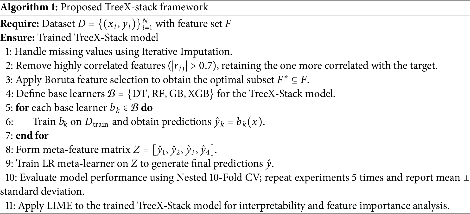
In this section, the proposed model is described, and its general functionality is outlined. The pseudocode of the algorithm is as shown in Algorithm 1 below. The first phase is data preprocessing, which addresses missing values using the Iterative Imputation method. The Boruta feature selection technique is then applied to select the most important features. Next, the TreeX-Stack model is constructed. Nested CV with 10 folds is used to ensure that model performance is evaluated accurately and fairly. Each experiment is repeated five times, and the mean performance along with the standard deviation is reported. Finally, LIME is employed to analyze model predictions and understand the contribution of individual features. Further details of each step are provided in the following sections.
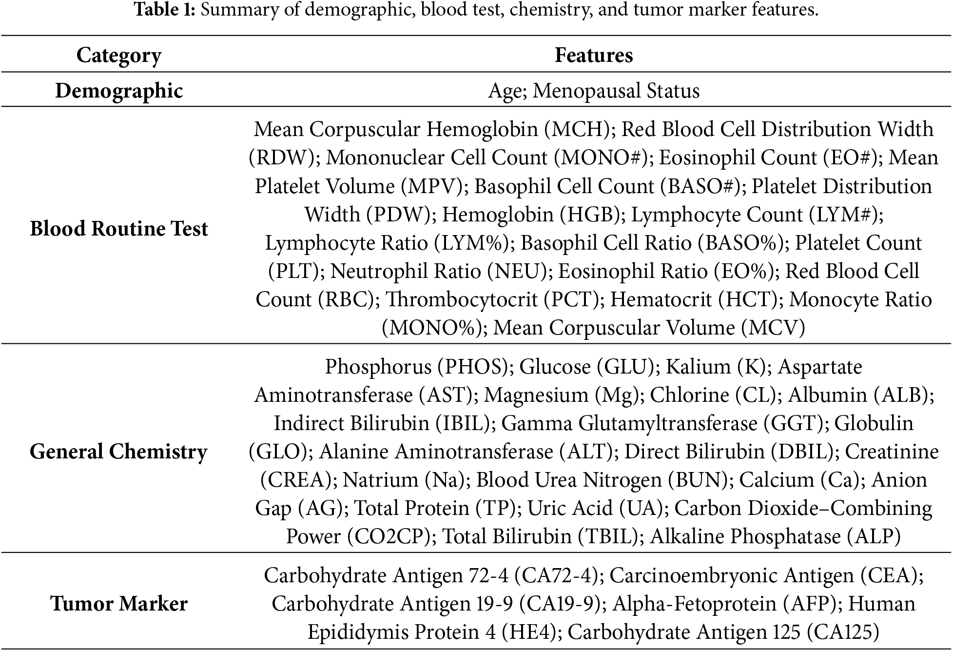
The dataset used in this study consisted of patients who underwent surgical resection at the Third Affiliated Hospital of Soochow University between July 2011 and July 2018. It includes data from 349 individuals, comprising 171 OC patients and 178 patients with benign ovarian tumors. Among the OC cases, 157 were Epithelial OC, 5 were Ovarian Germ Cell Cancer, and 9 were classified as other types. The benign tumor group includes 36 Ovarian Teratoma and 142 Ovarian Cyst cases. No OC patients were given radiation or chemotherapy before surgery; all patients were diagnosed by postoperative pathology. The dataset contains 49 features, including demographic data, blood routine test, general chemistry test, and tumor markers. A detailed list of these features is provided in Table 1. The dataset is publicly available through the Mendeley Data repository, allowing access for research purposes [32].
In healthcare, datasets typically have problems, including missing values, multicollinearity, and features that aren’t useful, all of which can make predictive modeling less accurate and less efficient. So, preparing data is important to make it more accurate and reliable. Fig. 1 shows that a large number of values were missing. The feature CA 72-4 has about 69% missing data, hence it was taken out of the dataset. The NEU feature has about 26% missing values; however, all other features had less than 10% missing data. There were no missing values in the target variable.
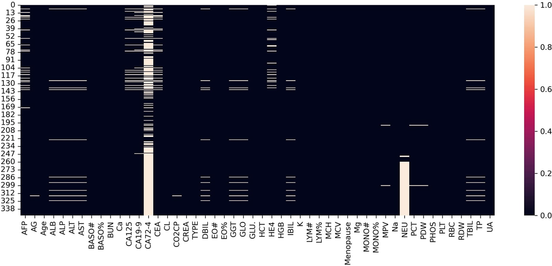
Figure 1: The missing values.
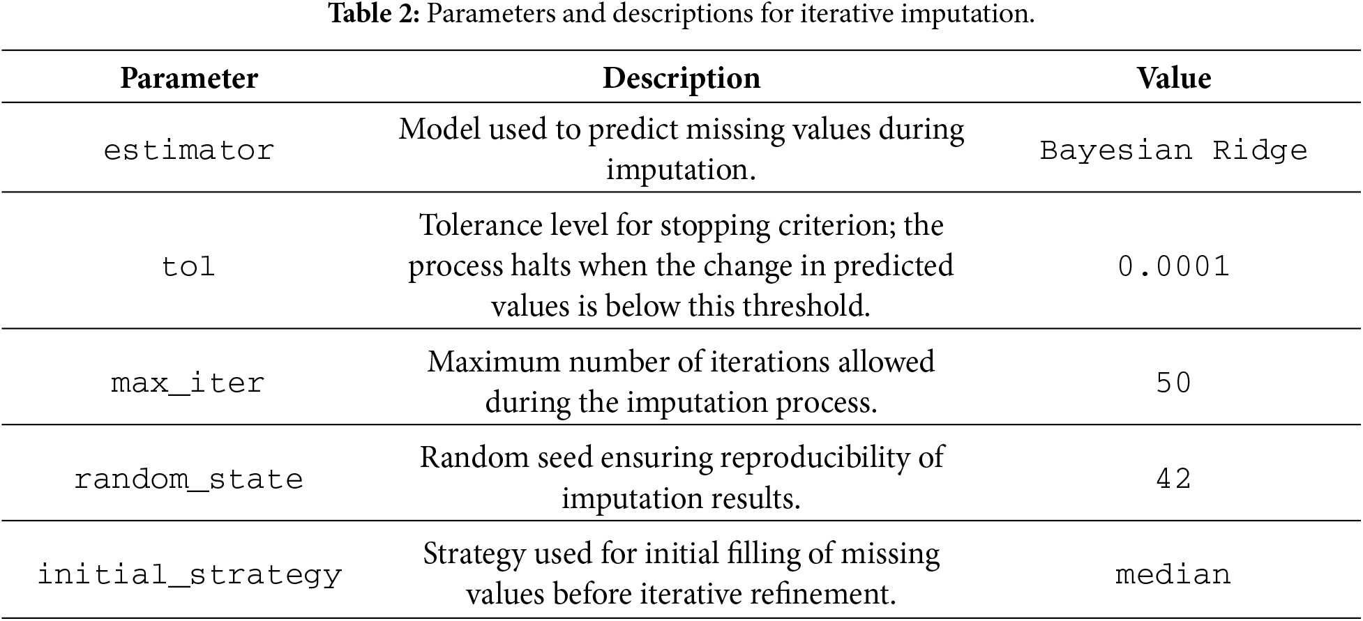
After taking out CA 72-4, the other missing values were imputed using iterative imputation. This method treats each feature with missing data as a function of the other features in the dataset, and it keeps improving the predicted values to make them more accurate. During imputation, Bayesian Ridge was utilized to make an estimate. Table 2 shows a summary of the settings and parameters for the imputation procedure.
3.3 Feature Reduction and Selection
Feature selection is an important part of ML that helps models work better by getting rid of unnecessary and duplicate features [43]. The dataset still had 47 features after the CA 72-4 feature was taken out. Some of these features exhibited multicollinearity, where two or more features are highly correlated, which can make model training less stable and reduce interpretability. To resolve this issue, the Pearson correlation coefficient was utilized to measure the linear relationship between pairs of characteristics. The Pearson correlation coefficient (
where the covariance between X and Y is denoted by
After addressing multicollinearity, the feature set was further refined using an automated feature selection method Boruta. The Boruta algorithm is a robust wrapper-based method built on tree-based model [44]. It creates “shadow” features by shuffling the original features and then uses a tree-based model to estimate their importance. In this study, RF model was used to compute the Z-score of feature importance for both original and shadow features. Features with higher importance scores than their shadow features were retained, while less informative features were discarded.
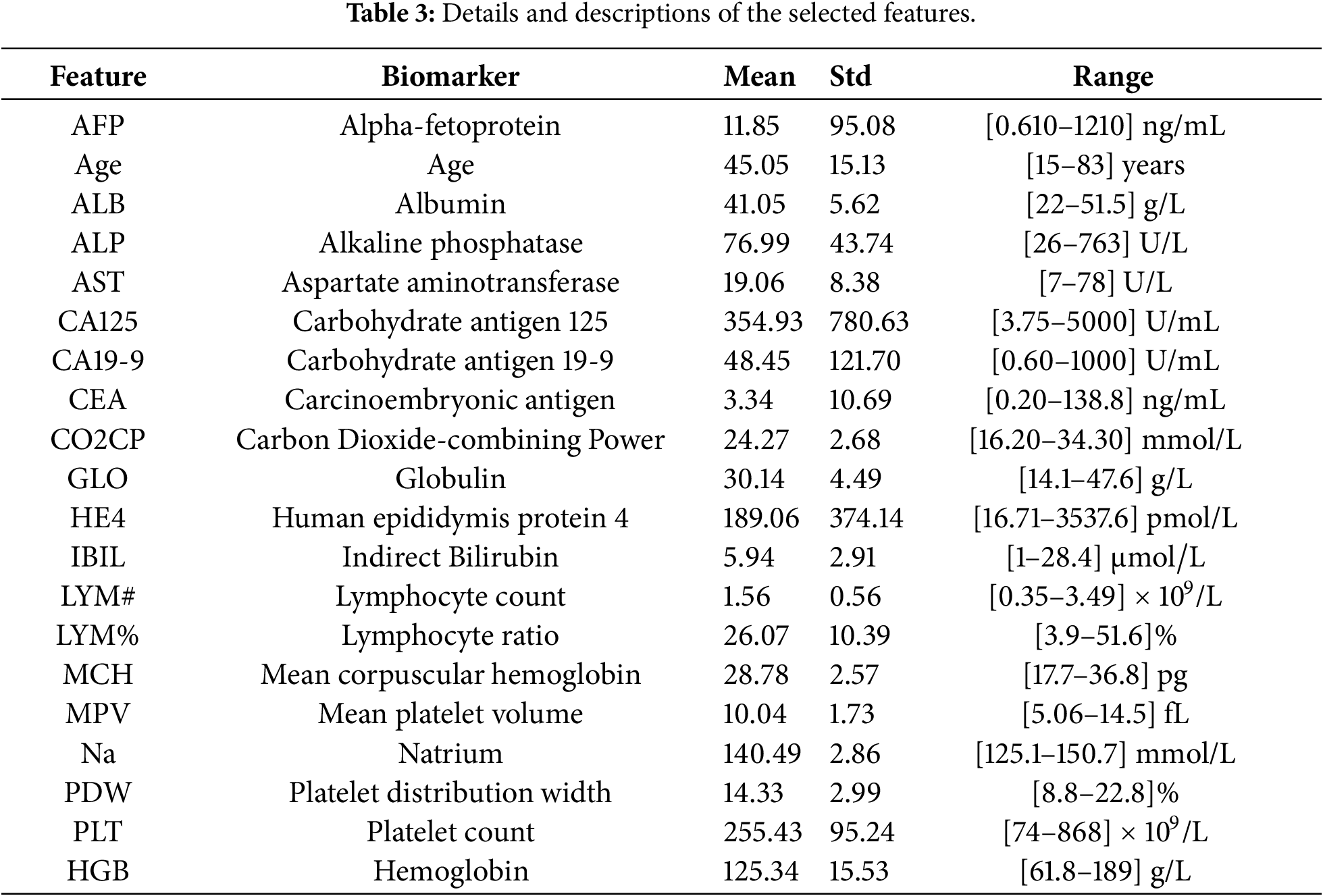
The Boruta algorithm rejected 17 features, leaving 20 features for further analysis. Subsequent modeling and evaluation were performed using these selected 20 features. A summary of the retained features and their statistical properties is presented in Table 3.
The correlation heatmap of the selected features is shown in Fig. 2, illustrating the correlation of each feature with the target variable TYPE, which has two classes: 1 for benign ovarian tumors and 0 for OC. The matrix indicates that there is no significant multicollinearity among the selected features.
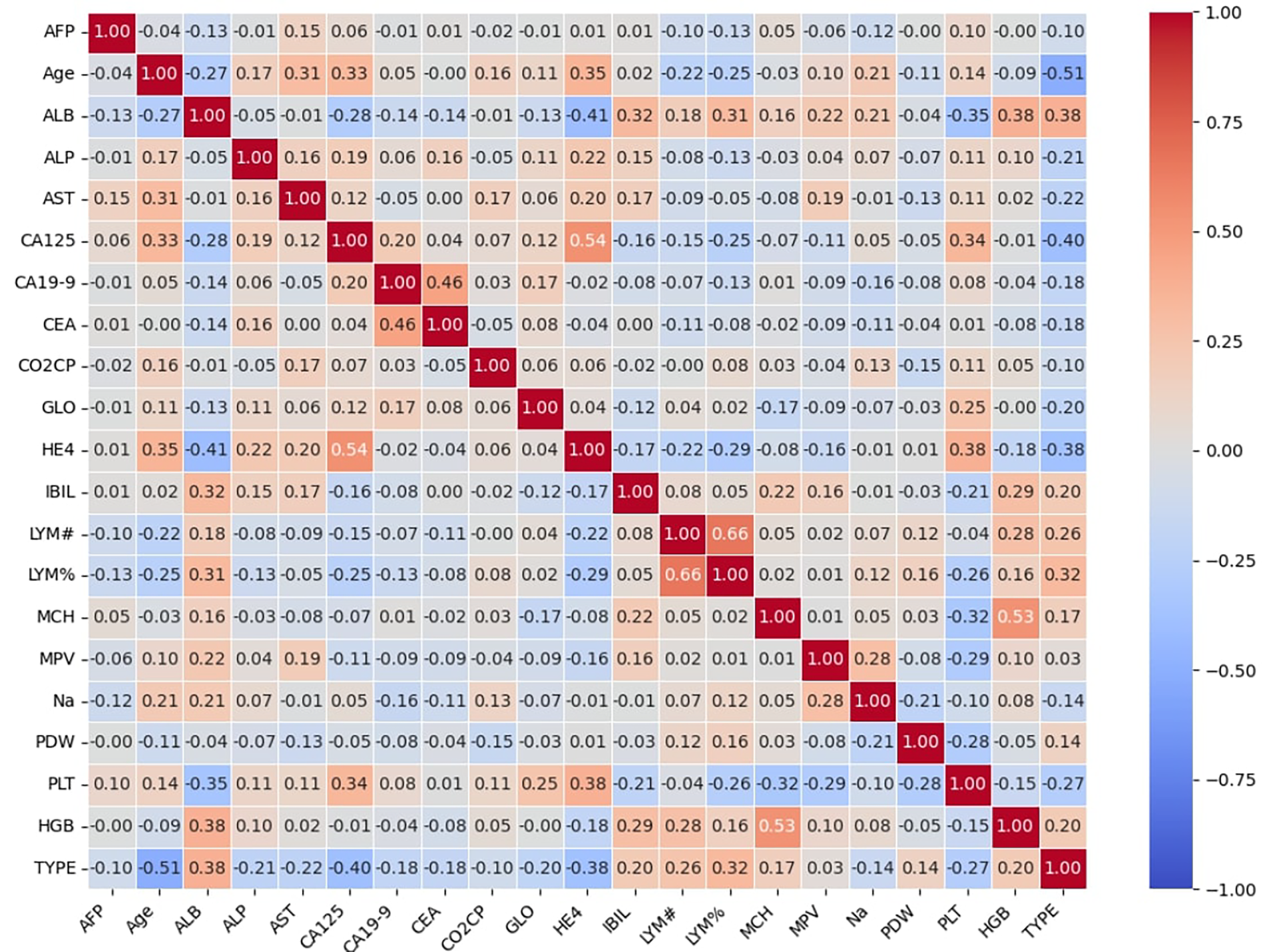
Figure 2: The correlation heatmap of selected features.
The proposed TreeX-Stack model utilizes tree-based classifiers as base learners, including DT, RF, GB, and XGBoost. Tree-based algorithms are particularly well-suited for biomedical data because they can capture complex nonlinear relationships among features, handle multicollinearity effectively, and remain robust in the presence of outliers. LR serves as the meta-model, integrating and refining the predictions of the base learners to generate the final classification. Fig. 3 illustrates the architecture of the proposed model.
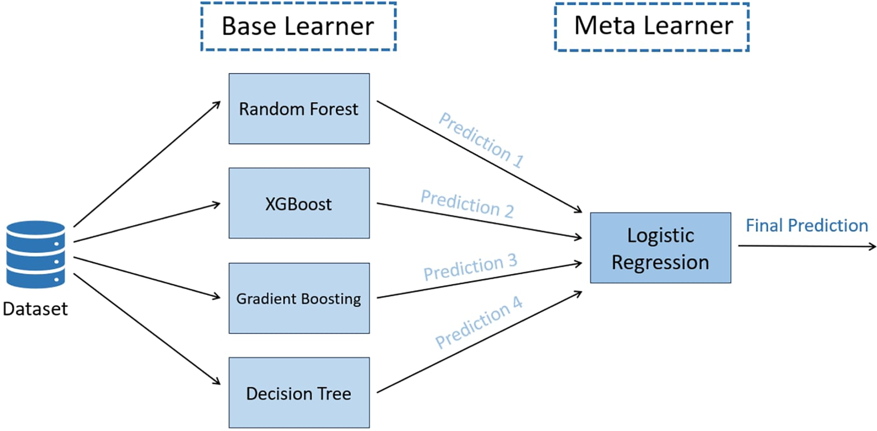
Figure 3: Proposed TreeX-Stack architecture.
The first base model, DT, has a tree-like structure with a root node, internal nodes, branches, and leaf nodes. The dataset is split up into smaller parts over and over again based on the most useful features, which are found using measures like gini impurity or entropy. The equations for these metrics of impurity are:
Here,
The second model, RF, makes a group of DT, each trained on a different set of attributes and samples. This randomization makes the model more stable and less likely to overfit. The last prediction comes from voting for classification across all trees [45].
The third base learner, GB, builds trees sequentially, where each new tree attempts to correct the errors made by the previous ensemble [46]. The contribution of each tree is scaled by a learning rate (
where
The last base model, XGBoost, is an advanced version of GB known for its scalability and strong regularization techniques [47]. It includes L1 and L2 penalties to reduce overfitting and enhance generalization. The objective function of XGBoost is defined as:
where L denotes the loss function,
Here, T denotes the number of leaves,
The meta-classifier used in the proposed framework is LR, which predicts the probability that an instance belongs to a particular class using the sigmoid activation function. The sigmoid function is defined as:
LR was chosen as the meta-classifier because it combines the predictions of base models in a simple, understandable, and strong method that doesn’t lead to overfitting. This is because it has few parameters and built-in regularization. The final classification result comes from the LR model after the tree-based base learners make their predictions and send them to it.
3.5 Experimental Evaluation Setup
This section discusses the experimental setting used to evaluate the performance of the proposed model. The assessment employs a nested CV strategy with 10 folds. Grid search is applied in the inner loop to optimize the hyperparameters, while the outer loop evaluates the generalization performance of the optimized model. Each experiment is repeated five times to ensure robustness and reduce variability caused by random data splits. The final performance is reported as the mean and standard deviation of the evaluation metrics.
Accuracy, precision, recall, and F1-score are used to evaluate the TreeX-Stack model. These metrics employ True Positives (TP), True Negatives (TN), False Positives (FP), and False Negatives (FN). These metrics are mathematically defined below:
To evaluate a model’s performance, the dataset may be split into training and test subsets. Nevertheless, using a single random split may yield biased or unstable results, as the outcome may vary substantially depending on how the data are divided. This issue is commonly addressed using K-fold CV. In this technique, the dataset is divided into
• Outer loop: Splits the dataset into
• Inner loop: Performs hyperparameter optimization within the training data of the outer loop to identify the best model parameters.
Nested CV is employed in this study to obtain robust performance estimates. In the outer loop, the dataset is divided into 10 folds, and in each iteration, one fold is used for testing while the remaining folds are used for training. The inner loop performs grid search CV on the training folds to optimize the hyperparameters. The results from each iteration of the outer loop are averaged, and the entire process is repeated five times. The overall performance is reported as the mean and standard deviation of these five runs, providing a reliable and generalizable estimate of the model’s performance.
3.5.3 Hyperparameter Optimization
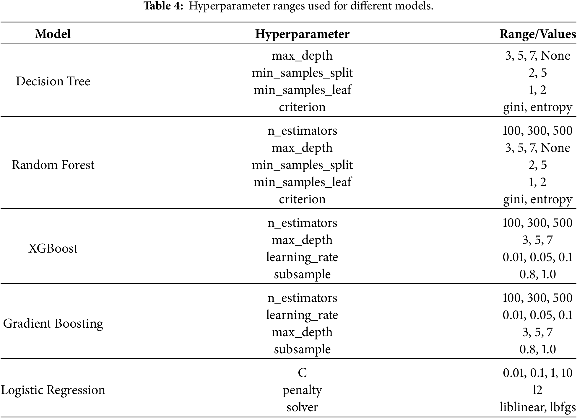
To improve the model’s performance, hyperparameter optimization plays a significant role. It refers to the process of selecting hyperparameter values that optimize model performance on the dataset. One of the most commonly used methods is Grid Search. This method systematically evaluates all possible combinations of hyperparameter values to identify the optimal configuration within the defined search grid [49]. In this research, nested CV with 10 folds is employed, where hyperparameter optimization is performed using Grid Search in each inner loop. The best hyperparameter combination from each fold is selected and used to train the model. Table 4 presents the ranges of hyperparameters explored for each model.
3.6 Explainability and Model Interpretation
The interpretation of the TreeX-Stack model is challenging due to its complexity, which includes a meta-classifier and several base learners. Explainability is essential in clinical settings because medical personnel must understand how and why the model produces a particular prediction [50]. To address this issue, the model incorporates LIME, an explainable AI approach. LIME approximates the complex model locally using a simple and interpretable model in order to explain individual predictions [51]. The mathematical formulation for an observation
where H denotes the set of interpretable models,
LIME is model-agnostic, meaning it can be applied to any ML model. It generates perturbed samples around
All experiments were conducted on an HP ZBook 15 G6 mobile workstation equipped with an Intel Core i9-9880H processor, 32 GB of DDR4 RAM, and a 512 GB SSD. Python was chosen for model development and analysis because of its extensive library support and ease of use. Several Python libraries were used to develop and evaluate the proposed TreeX-Stack framework. Mathematical computation, visualization, and plotting of data were performed using standard libraries such as NumPy, Pandas, seaborn, and Matplotlib. Boruta library was used for feature selection, and scikit-learn was used for model implementation, nested CV, and hyperparameter tunning of the model. The XGBoost library was used to implement the XGBoost model. For model explainability, the LIME library was utilized.
In this study, a diagnostic model for OC is proposed, namely TreeX-Stack. It is a model based on a stacking ensemble with several tree-based base models, such as DT, RF, GB, and XGBoost, and LR is the meta-classifier. The dataset originally contains 49 features. To address multicollinearity, features associated with the target variable by more than 0.7 were excluded. Subsequently, Boruta feature selection was applied to identify the most important features, yielding a subset of 20 features for model training.
We used a nested 10-fold CV with grid search to optimize the model’s hyperparameters and assess its performance. The proposed TreeX-Stack model achieved strong performance in classifying OC and benign ovarian tumors, with an accuracy of 0.9027
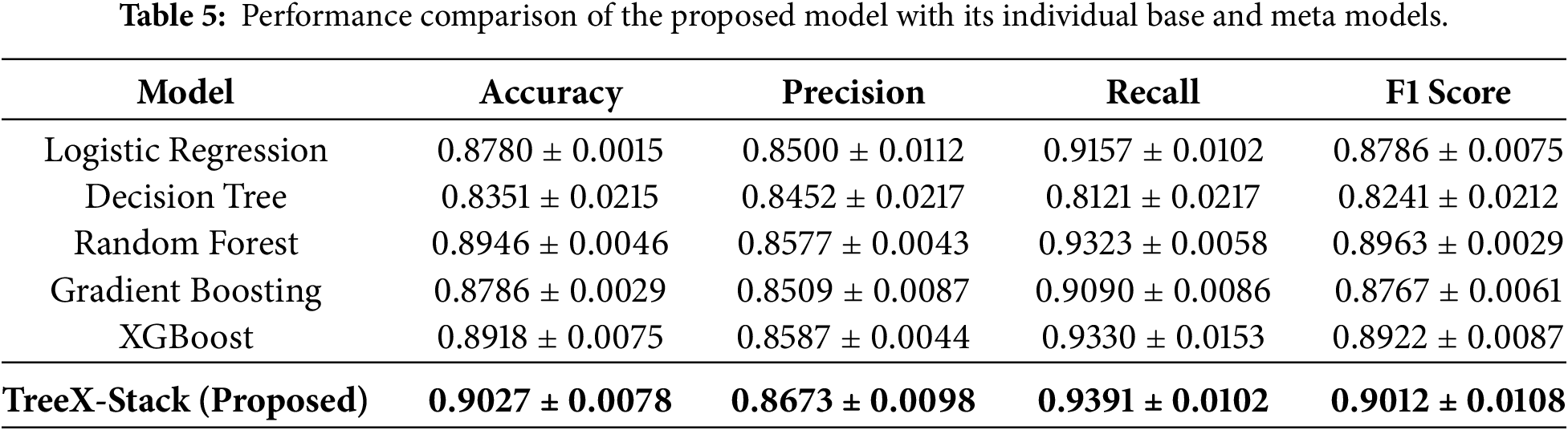
The results indicate strong potential of the proposed model to accurately classify OC and benign ovarian tumors. The TreeX-Stack model was also compared with its individual base models and the meta-classifier alone, applying the same preprocessing steps. As shown in Table 5, the proposed model outperformed all individual models in terms of all evaluated metrics.
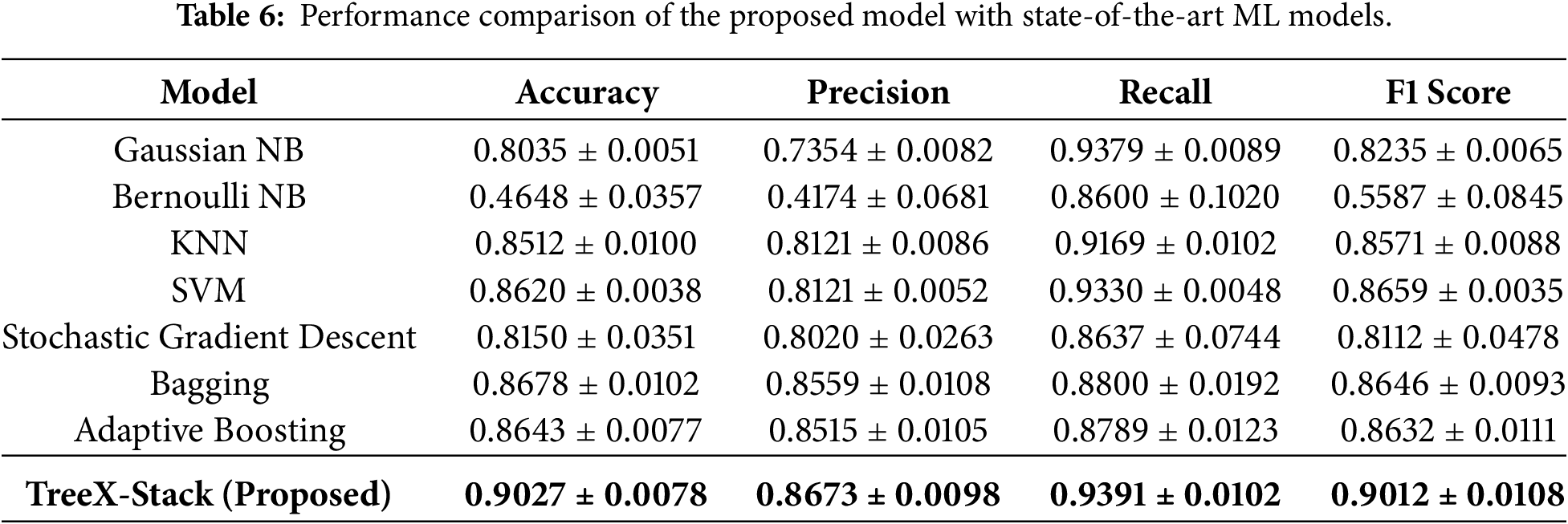
Additionally, the proposed TreeX-Stack model was compared with various state-of-the-art models, including Gaussian NB, Bernoulli NB, Stochastic Gradient Descent, KNN, SVM, Bagging and Adaptive Boosting. Table 6 shows the results, which show that the proposed model does better than these models in all of the metrics.
To further evaluate the proposed model, curve-based performance analysis was conducted, including the receiver operating characteristic (ROC) curve, precision–recall (PR) curve, calibration curve and decision curve.
The area under the ROC curve (AUC-ROC) measures the ability of model to distinguish the OC tumors from benign ovarian tumors across different thresholds. As shown in Fig. 4a, the ROC curve of the proposed model demonstrates strong discriminative capability, achieving an AUC-ROC score of 0.952. The PR curve illustrates the trade-off between precision and recall at varying thresholds. As depicted in Fig. 4b, the proposed model achieved a PR AUC of 0.935, indicating that the model maintains high precision while effectively capturing positive OC cases. The strong performance observed in both curves demonstrates the robustness and reliability of the proposed model in distinguishing OC tumors from benign ovarian tumors.
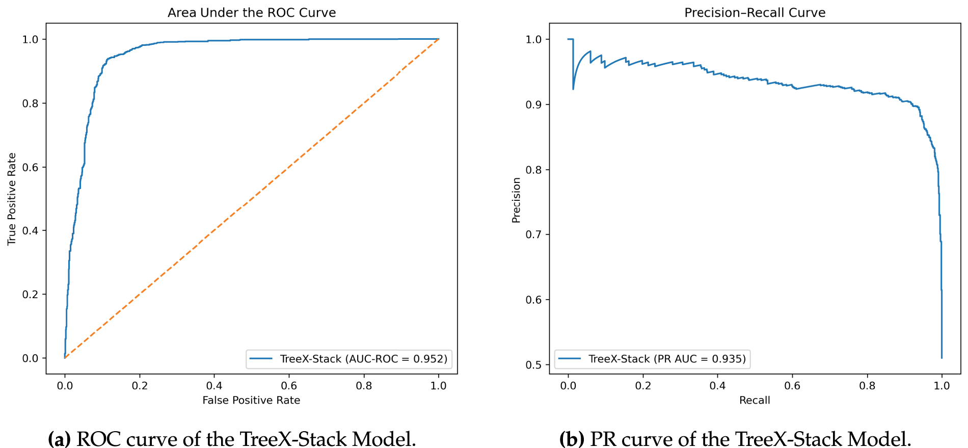
Figure 4: ROC and PR curves of the TreeX-Stack model.
The calibration curve of the proposed TreeX-Stack model for classifying OC vs. benign tumors is shown in Fig. 5. The x-axis represents the predicted probabilities output by the model, while the y-axis shows the corresponding true probabilities (fraction of positive cases) in each bin. The dashed diagonal line represents perfect calibration, where predicted probabilities exactly match observed outcomes. The curve indicates that the model is overconfident for predicted probabilities between 0 and 0.4, reasonably well-calibrated in the range 0.4–0.6, and under-confident between 0.6 and 0.85. Near predicted probabilities of 0.9–1.0, the curve flattens, suggesting that very high predicted probabilities correspond to true probabilities of around 0.9. Overall, the TreeX-Stack model demonstrates satisfactory calibration, providing reliable probability estimates for differentiating ovarian cancer from benign tumors.
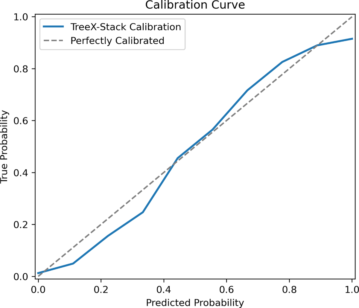
Figure 5: Calibration curve of the TreeX-Stack model
Decision curve is used to evaluate the clinical usefulness of predictive models, diagnostic tests, or risk scores, considering the net benefit of using a model in a clinical decision-making context [52]. The net benefit can be calculated as
where TP is the number of true positives, FP is the number of false positives, N is the total number of patients, and
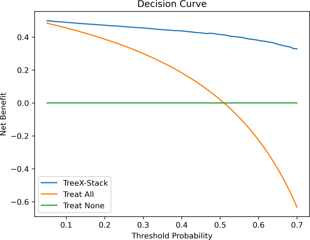
Figure 6: Decision curve of the TreeX-Stack model.
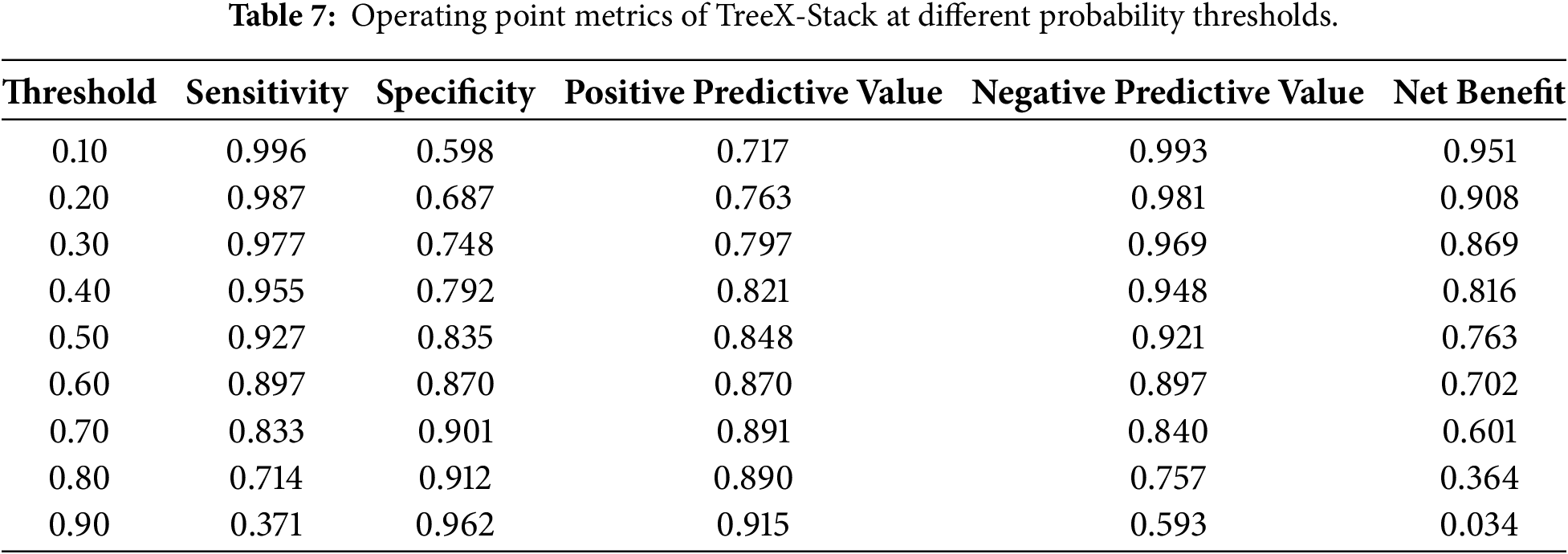
Table 7 presents the operating-point values of the TreeX-Stack model across various probability thresholds. The sensitivity of the model is very high (at low thresholds, 0.10–0.30) since most cases of OC are identified, but the specificity is moderate (high false positives). The net benefit is maximized at these levels, indicating a high degree of clinical usefulness in circumstances where cancer detection is a priority. The range (0.40–0.60) offers a balance between sensitivity and specificity, with a substantial net benefit and minimal unnecessary interventions; therefore, it is a more realistic range for use in real-world decision-making. Beyond the high thresholds (0.70–0.90), sensitivity reduces significantly, net benefit declines, and despite the high specificity, a large proportion of true cancers will be missed, decreasing clinical utility.
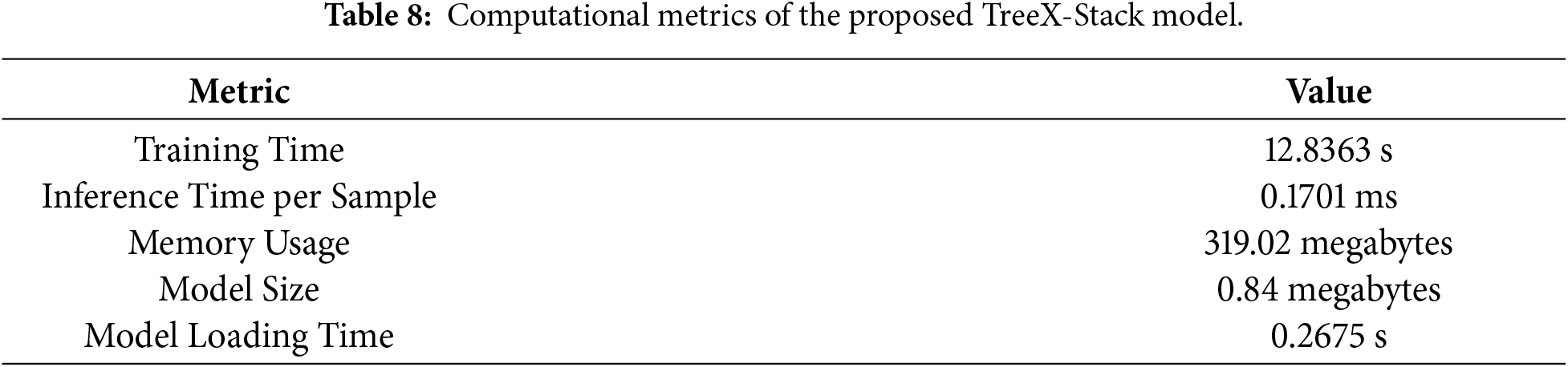
Along with the predictive performance, it is necessary to estimate the computational cost of the TreeX-Stack model. Stacking has higher computational requirements than individual base models; therefore, these measures can be used to assess the viability of implementing the model on edge devices or in low-resource clinical settings. The model was trained using the entire 349-sample dataset. The training time, or the time taken by the model to train on the entire dataset, was 12.8363 s. The time of inference per sample, which is the time taken to make a prediction with one input, was 0.1701 ms. This was estimated by summing the total inference time across all samples and dividing by the number of samples, yielding an average per-sample inference time. The value is low, indicating that the model can make rapid predictions. Memory usage was 319.02 megabytes, representing the amount of RAM required to execute the model. The model size, representing the disk space required to store the trained model, was 0.84 megabytes. Finally, the model loading time, defined as the time required to load the model from disk into memory, was 0.2675 s. These computational metrics, summarized in Table 8, demonstrate that the TreeX-Stack model is efficient and suitable for deployment in resource-limited clinical environments.
Explainability is crucial for understanding complex ML models, particularly in the medical domain, where it is important to know why a model produces a specific prediction. The TreeX-Stack model combines several tree-based learners with LR as a meta-learner, which makes the model inherently complex. Without interpretability, such a model would have limited usefulness in clinical decision-making. To address this issue, the LIME technique is employed to provide explainability for the proposed system.
Fig. 7 shows a LIME explanation for a sample predicted as a benign ovarian tumor. The right side of the figure displays the contributing features along with their values: features highlighted in orange support the benign tumor prediction, while those highlighted in blue support OC. The left side presents the model’s output, indicating a predicted probability of 92% for the benign class. The middle panel visualizes the local decision boundary of the model, showing that features such as HE4 and AFP strongly support the benign diagnosis, whereas CA19-9 contributes toward malignancy.
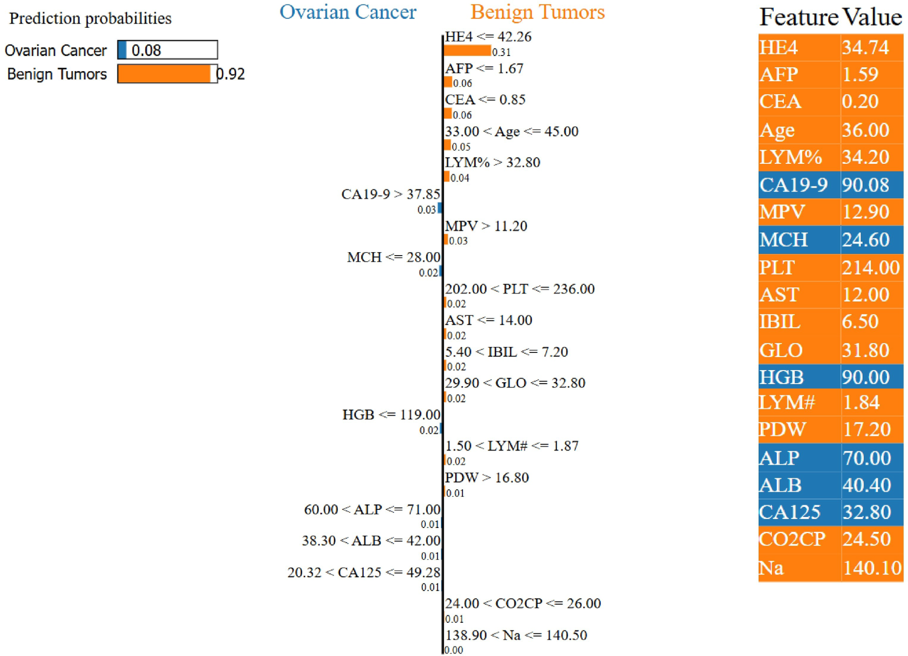
Figure 7: Example of a LIME-based explanation for a patient diagnosed with a benign ovarian tumor by the proposed TreeX-Stack model.
Fig. 8 presents a LIME explanation for a patient diagnosed with OC. The right side of the figure shows the contributing features and their values: features highlighted in yellow support benign tumor prediction, while those in blue support OC prediction. The left panel displays the model output, indicating an 86% predicted probability for OC. The central panel visualizes the model’s decision boundary, showing that features such as CA125, CEA, and MCH strongly support malignancy, whereas HE4 contributes toward a benign diagnosis.
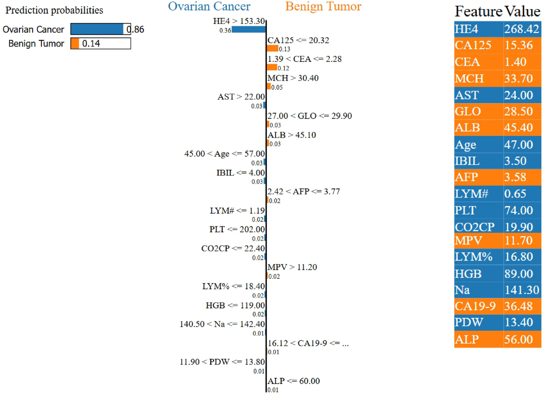
Figure 8: Example of a LIME-based explanation for a patient diagnosed with OC by the proposed TreeX-Stack model.
While LIME is primarily designed to provide local explanations for individual predictions, it can also be extended to offer global interpretability by aggregating feature importance across multiple instances. By averaging the importance weights of all samples, a global view of the model’s behavior can be obtained. Fig. 9 presents the global feature importance derived from LIME, revealing that HE4, CEA, CA125, and Age are the four most influential biomarkers, in that order.
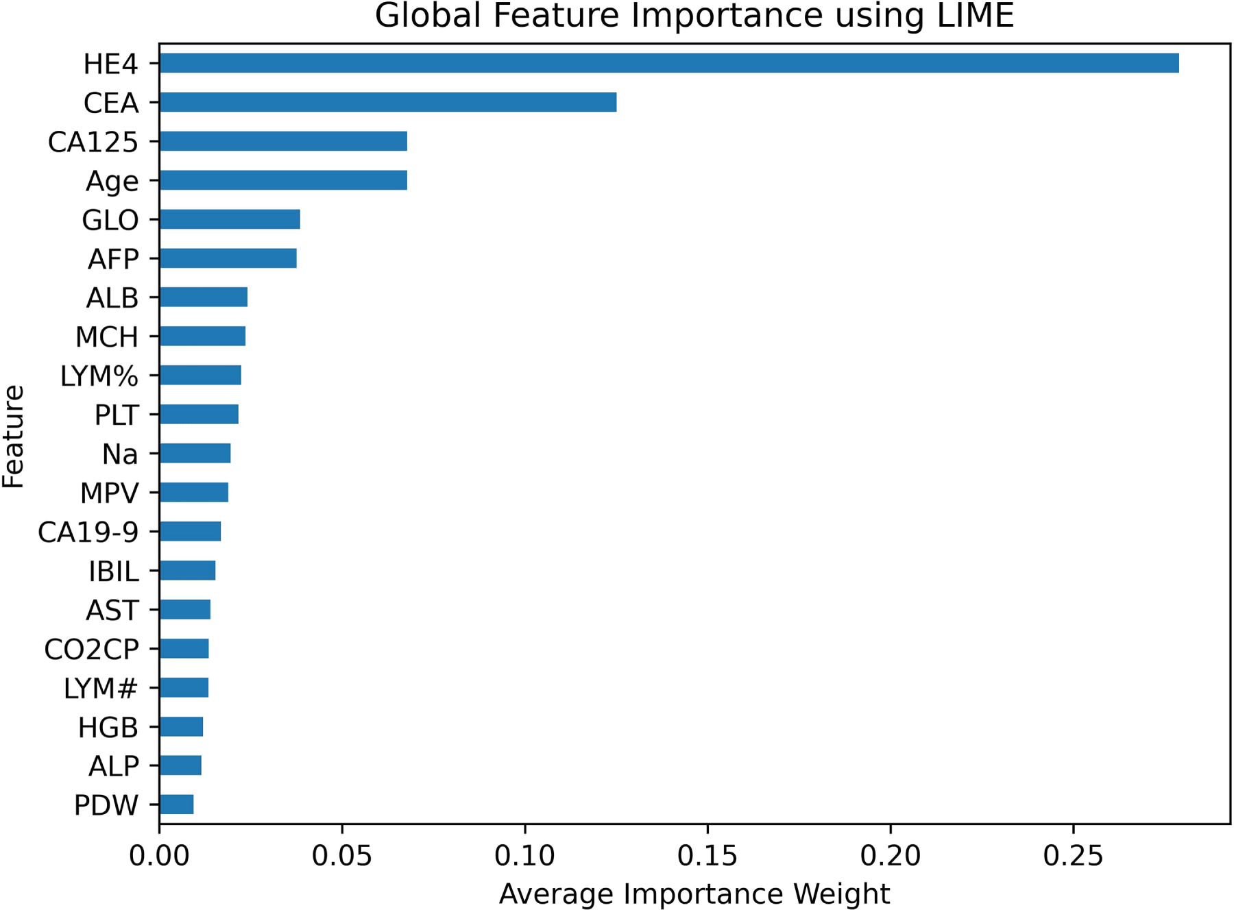
Figure 9: Global feature importance using LIME.
In addition to LIME, permutation feature importance was employed to further assess the contribution of each feature to the model’s performance. This method evaluates the impact of a feature by randomly shuffling its values and observing the corresponding drop in model performance. A larger drop in performance means that the feature is more important. The F1 score served as the evaluation tool for permutation importance in this study. The plot in Fig. 10 shows that HE4, CEA, CA125, and GLO are the most important traits in order of relevance.
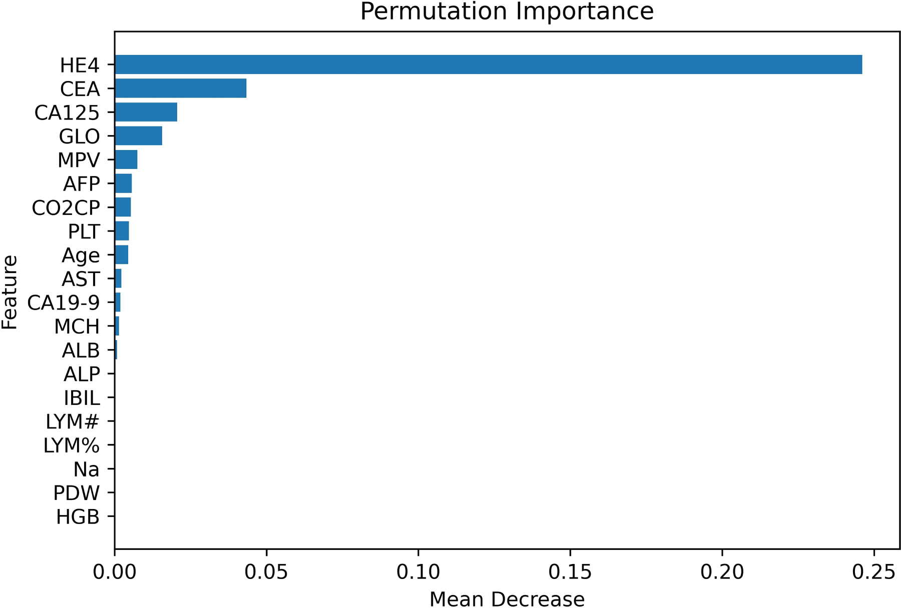
Figure 10: Permutation-based feature importance.
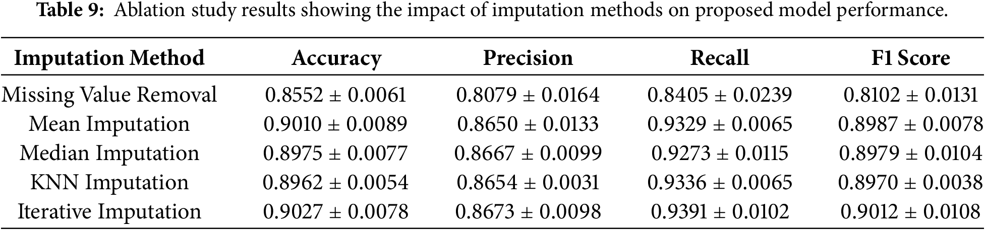
An ablation study was conducted to assess the contribution of individual components of the proposed framework. The dataset initially contained 49 features; however, the CA72-4 feature was removed prior to imputation due to its high missing rate (69%), resulting in 48 remaining features. An ablation analysis was then performed to evaluate the impact of different imputation methods. As a baseline, all samples with missing values were removed. Subsequently, several imputation techniques were applied, including mean and median imputation, KNN imputation, and iterative imputation. The results of this analysis are presented in Table 9. The findings indicate that applying imputation substantially improves the model’s performance compared to removing missing values. Although the differences among the imputation methods are relatively small, all imputation techniques yield comparable performance, with iterative imputation achieving slightly superior results.
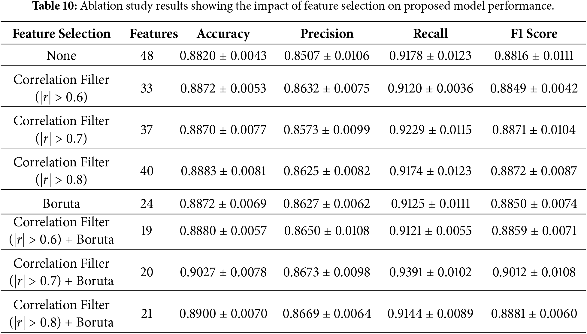
Next, an ablation study was conducted to evaluate the effect of feature selection on the proposed model. After removing the CA72-4, the dataset contained 48 features. Since many features exhibited multicollinearity, a correlation-based filter was applied to remove redundant features, followed by Boruta feature selection to identify the most relevant predictors. Several experiments were performed. First, the model was evaluated without applying any feature selection. Next, correlation filtering was applied using different thresholds (
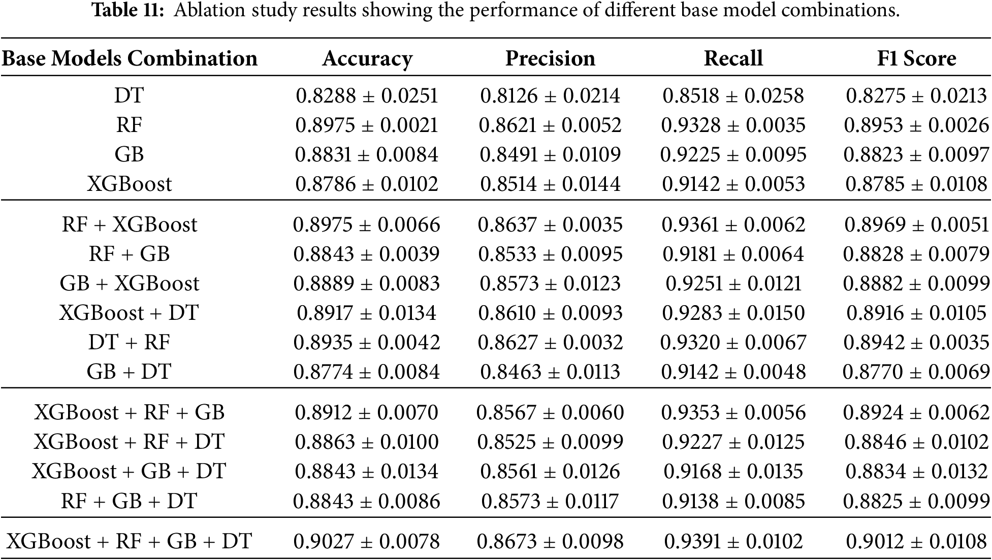
After the feature selection analysis, another ablation research was done to find out how each base model in the TreeX-Stack architecture contributed to the overall model. This entailed the methodical elimination of particular base learners, DT, RF, GB, and XGBoost, to evaluate their distinct influence on overall performance. We did experiments with single models, pairs of models, and groups of models, always using LR as the meta-learner. Table 11 shows the findings of this base model ablation study, which shows how well different base model configurations work within the framework.
Worldwide, OC is among the most frequent malignancies affecting females. A clinical evaluation, which includes looking at the patient’s medical history, symptoms, and physical exam, is the most typical way to diagnose it. Medical imaging, laboratory testing, and pathological investigations, including blood tests, biochemical analyses, and tumour marker evaluations, are also utilized for diagnosis. Traditional approaches work, but they are time-consuming, expensive, and rely on expert interpretation. The exponential rise of medical data has allowed ML to be used in healthcare in new ways in recent decades. ML algorithms may identify complex data patterns and assist individuals predict outcomes. Use of ML in medicine is problematic since it functions like a “black box,” making predictions without explanation. It is difficult to employ in therapeutic practice, since trust and openness are crucial for excellent decisions.
This study used clinical data, including demographics, blood tests, and chemistry results. This dataset was cleaned by removing feature CA 72-4, which contained 69% missing values. Bayesian Ridge regression was then used to impute the remaining missing data. To address multicollinearity, 11 features with a correlation coefficient greater than 0.7 were removed. Boruta feature selection with a RF estimator was subsequently applied to identify 20 essential features for further analysis and model development. The proposed TreeX-Stack model is built using a stacking EL approach, with DT, RF, GB, and XGBoost as base learners, and LR as the meta-model. A 10-fold nested CV was employed to evaluate model performance, where the outer loop divided the data into 10 folds, and the inner loop performed grid search for optimal hyperparameter tuning. Mean performance metrics were reported after repeating each experiment five times.
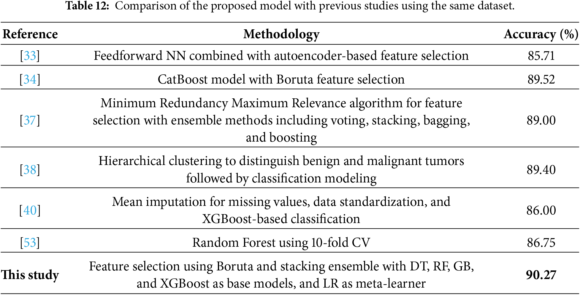
The proposed model achieved an accuracy of 0.9027
The proposed model has a complex structure, which makes it difficult to interpret, even if it performs well in making predictions. Explainability is particularly important in clinical contexts, as physicians need to understand why a model produces certain predictions to trust it and communicate its results transparently. To address this, we employed LIME, which provides instance-level explanations by quantifying the contribution of each feature to individual predictions. This enhances the model’s utility in clinical decision-making.
LIME was employed to provide both local interpretability and global feature importance analysis, complemented by permutation feature importance to further validate the findings. Both approaches consistently identified HE4, CEA, and CA125 as the most important biomarkers. Prior research clearly supports these conclusions. For example, Öznacar and Güler identified HE4 and CA125 as key features [34], Sheela Lavanya and Subbulakshmi identified HE4 and NEU [37], Jamalpour et al. identified age, CA125, HE4, and CA19–9 as key predictors [38], Abuzinadah et al. identified HE4, NEU, and CA125 [39], and Ahamad et al. identified CA19–9, CE, and HE4 [40]. The consistent identification of HE4 across studies highlights its role as a key biomarker for OC diagnosis, while variations in other features likely reflect differences in preprocessing, imputation, feature selection, and modeling strategies.
LIME allows clinicians to intuitively understand which biomarkers influence predictions, thereby increasing confidence in risk assessment. The TreeX-Stack model can provide both predictions and explanations to support clinical decision-making without requiring changes to the standard workflow.
The study proposed TreeX-Stack, an explainable diagnosis model for OC. The model comprises a stacked ensemble with DT, RF, GB, and XGBoost as base classifiers and LR as the meta-classifier. The dataset comprises 49 features, including demographic data, blood routine test results, general chemistry, and tumor markers. Missing values were imputed using iterative imputation with Bayesian ridge, and highly correlated features were removed to address multicollinearity. The Boruta feature selection algorithm identified 20 significant features, which were used for model development. The proposed model achieved good performance, with an accuracy of 0.9027
Despite the use of nested CV to mitigate overfitting, the relatively small, single-center dataset and model complexity still present a risk of overfitting, which may affect generalizability to external cohorts. Future research will focus on expanding the dataset with larger and more heterogeneous samples, exploring DL models, and developing a web-based clinical tool capable of providing real-time predictions along with model explanations to support informed decision-making. Additionally, the development of real-time web or mobile clinical applications with built-in explainability features may facilitate the translation of this research into routine clinical practice.
Acknowledgement: This research was supported and funded by the Deanship of Scientific Research, Imam Mohammad Ibn Saud Islamic University (IMSIU), Saudi Arabia.
Funding Statement: This work was supported and funded by the Deanship of Scientific Research at Imam Mohammad Ibn Saud Islamic University (IMSIU) grant number IMSIU-DDRSP2601.
Author Contributions: Daniyal Asif: conceptualization, methodology, software, formal analysis, data curation, visualization, validation, writing—original draft preparation; Nabil Kerdid: supervision, project administration, resources, funding acquisition, writing—review and editing; Muhammad Shoaib Arif: methodology, validation, formal analysis, writing—review and editing; Mairaj Bibi: methodology, validation, formal analysis, writing—review and editing. All authors reviewed and approved the final version of the manuscript.
Availability of Data and Materials: The dataset used in this study is publicly available at Mendeley Data: https://data.mendeley.com/datasets/th7fztbrv9/11.
Ethics Approval: Not applicable.
Conflicts of Interest: The authors declare no conflicts of interest.
Abbreviations
| OC | Ovarian Cancer |
| ML | Machine Learning |
| AI | Artificial Intelligence |
| EL | Ensemble Learning |
| LIME | Local Interpretable Model-Agnostic Explanations |
| PCA | Principal Component Analysis |
| RFE | Recursive Feature Elimination |
| KNN | K-Nearest Neighbors |
| SVM | Support Vector Machine |
| LR | Logistic Regression |
| RF | Random Forest |
| NB | Naive Bayes |
| DL | Deep Learning |
| NN | Neural Networks |
| DT | Decision Tree |
| CV | Cross-Validation |
| SHAP | SHapley Additive exPlanations |
| AUC | Area under the curve |
| XGBoost | Extreme Gradient Boosting |
| GB | Gradient Boosting |
| ROC | Receiver Operating Characteristic |
| PR | Precision-Recall Curve |
| TP | True Positives |
| TN | True Negatives |
| FP | False Positives |
| FN | False Negatives |
References
1. Sung H, Ferlay J, Siegel RL, Laversanne M, Soerjomataram I, Jemal A, et al. Global cancer statistics 2024: GLOBOCAN estimates of incidence and mortality worldwide for 36 cancers in 185 countries. CA Cancer J Clin. 2024;74(2):123–52. [Google Scholar]
2. Siegel RL, Miller KD, Wagle NS, Jemal A. Cancer statistics 2023. CA Cancer J Clin. 2023;73(1):17–48. doi:10.3322/caac.21763. [Google Scholar] [PubMed] [CrossRef]
3. Matulonis UA, Sood AK, Fallowfield L, Howitt BE, Sehouli J, Karlan BY. Ovarian cancer. Nat Rev Dis Primers. 2016;2(1):1–22. doi:10.1038/nrdp.2016.61. [Google Scholar] [PubMed] [CrossRef]
4. Stewart C, Ralyea C, Lockwood S. Ovarian cancer: an integrated review. Semin Oncol Nurs. 2019;35(2):151–6. doi:10.1016/j.soncn.2019.02.001. [Google Scholar] [PubMed] [CrossRef]
5. Webb PM, Jordan SJ. Global epidemiology of epithelial ovarian cancer. Nat Rev Clin Oncol. 2024;21(5):389–400. doi:10.1038/s41571-024-00881-3. [Google Scholar] [PubMed] [CrossRef]
6. Momenimovahed Z, Tiznobaik A, Taheri S, Salehiniya H. Ovarian cancer in the world: epidemiology and risk factors. Int J Womens Health. 2019;11:287–99. doi:10.2147/ijwh.s197604. [Google Scholar] [PubMed] [CrossRef]
7. Clarke-Pearson DL. Screening for ovarian cancer. N Engl J Med. 2009;361(2):170–7. doi:10.1056/nejmcp0901926. [Google Scholar] [PubMed] [CrossRef]
8. Jacobs IJ, Menon U. Progress and challenges in screening for early detection of ovarian cancer. Mol Cell Proteomics. 2004;3(4):355–66. doi:10.1074/mcp.r400006-mcp200. [Google Scholar] [PubMed] [CrossRef]
9. Bates CK, Carroll N, Potter J. The challenging pelvic examination. J Gen Intern Med. 2011;26(6):651–7. doi:10.1007/s11606-010-1610-8. [Google Scholar] [PubMed] [CrossRef]
10. Miceli V, Gennarini M, Tomao F, Cupertino A, Lombardo D, Palaia I, et al. Imaging of peritoneal carcinomatosis in advanced ovarian cancer: CT, MRI, radiomic features and resectability criteria. Cancers. 2023;15(24):5827. doi:10.3390/cancers15245827. [Google Scholar] [PubMed] [CrossRef]
11. Charkhchi P, Cybulski C, Gronwald J, Wong FO, Narod SA, Akbari MR. CA125 and ovarian cancer: a comprehensive review. Cancers. 2020;12(12):3730. doi:10.3390/cancers12123730. [Google Scholar] [PubMed] [CrossRef]
12. Berek JS, Renz M, Kehoe S, Kumar L, Friedlander M. Cancer of the ovary, fallopian tube, and peritoneum: 2021 update. Int J Gynecol Obstet. 2021;155:61–85. doi:10.1002/ijgo.13878. [Google Scholar] [PubMed] [CrossRef]
13. Liberto JM, Chen SY, Shih IM, Wang TH, Wang TL, Pisanic TR. Current and emerging methods for ovarian cancer screening and diagnostics: a comprehensive review. Cancers. 2022;14(12):2885. doi:10.3390/cancers14122885. [Google Scholar] [PubMed] [CrossRef]
14. Wiens J, Shenoy ES. Machine learning for healthcare: on the verge of a major shift in healthcare epidemiology. Clin Infect Dis. 2018;66(1):149–53. doi:10.1093/cid/cix731. [Google Scholar] [PubMed] [CrossRef]
15. Zhang A, Xing L, Zou J, Wu JC. Shifting machine learning for healthcare from development to deployment and from models to data. Nat Biomed Eng. 2022;6(12):1330–45. doi:10.1038/s41551-022-00898-y. [Google Scholar] [PubMed] [CrossRef]
16. Kolla L, Parikh RB. Uses and limitations of artificial intelligence for oncology. Cancer. 2024;130(12):2101–7. doi:10.1002/cncr.35307. [Google Scholar] [PubMed] [CrossRef]
17. Paleyes A, Urma RG, Lawrence ND. Challenges in deploying machine learning: a survey of case studies. ACM Comput Surv. 2022;55(6):1–29. doi:10.1145/3533378. [Google Scholar] [CrossRef]
18. Mahajan P, Uddin S, Hajati F, Moni MA. Ensemble learning for disease prediction: a review. Healthcare. 2023;11(12):1808. doi:10.3390/healthcare11121808. [Google Scholar] [PubMed] [CrossRef]
19. Sadeghi Z, Alizadehsani R, Cifci MA, Kausar S, Rehman R, Mahanta P, et al. A review of explainable artificial intelligence in healthcare. Comput Electr Eng. 2024;118:109370. doi:10.2139/ssrn.4600029. [Google Scholar] [CrossRef]
20. Bharati S, Mondal MRH, Podder P. A review on explainable artificial intelligence for healthcare: why, how, and when? IEEE Trans Artif Intell. 2023;5(4):1429–42. doi:10.1109/tai.2023.3266418. [Google Scholar] [CrossRef]
21. Ebell MH, Culp MB, Radke TJ. A systematic review of symptoms for the diagnosis of ovarian cancer. Am J Prev Med. 2016;50(3):384–94. doi:10.1016/j.amepre.2015.09.023. [Google Scholar] [PubMed] [CrossRef]
22. Kobayashi H. Ovarian cancer in endometriosis: epidemiology, natural history, and clinical diagnosis. Int J Clin Oncol. 2009;14(5):378–82. doi:10.1007/s10147-009-0931-2. [Google Scholar] [PubMed] [CrossRef]
23. Mathieu KB, Bedi DG, Thrower SL, Qayyum A, Bast RC Jr. Screening for ovarian cancer: imaging challenges and opportunities for improvement. Ultrasound Obstet Gynecol. 2018;51(3):293–302. doi:10.1002/uog.17557. [Google Scholar] [PubMed] [CrossRef]
24. Engbersen MP, Van Driel W, Lambregts D, Lahaye M. The role of CT, PET-CT, and MRI in ovarian cancer. Br J Radiol. 2021;94(1125):20210117. [Google Scholar] [PubMed]
25. Matsas A, Stefanoudakis D, Troupis T, Kontzoglou K, Eleftheriades M, Christopoulos P, et al. Tumor markers and their diagnostic significance in ovarian cancer. Life. 2023;13(8):1689. doi:10.3390/life13081689. [Google Scholar] [PubMed] [CrossRef]
26. Zhang R, Siu MKY, Ngan HYS, Chan KKL. Molecular biomarkers for the early detection of ovarian cancer. Int J Mol Sci. 2022;23(19):12041. doi:10.3390/ijms231912041. [Google Scholar] [PubMed] [CrossRef]
27. Habchi Y, Kheddar H, Himeur Y, Belouchrani A, Serpedin E, Khelifi F, et al. Machine learning and transformers for thyroid carcinoma diagnosis. J Vis Commun Image Represent. 2025;115:104668. doi:10.1016/j.jvcir.2025.104668. [Google Scholar] [CrossRef]
28. Habchi Y, Kheddar H, Himeur Y, Belouchrani A, Serpedin E, Khelifi F, et al. Advanced deep learning and large language models: comprehensive insights for cancer detection. Image Vis Comput. 2025;157:105495. doi:10.1016/j.imavis.2025.105495. [Google Scholar] [CrossRef]
29. El Ogri O, Jaouad EM, Hjouji A. A computer-assisted medical diagnosis system for cancer diseases based on quaternion orthogonal Rademacher-Fourier moments and deep learning. Biomed Signal Process Control. 2026;112:108744. doi:10.1016/j.bspc.2025.108744. [Google Scholar] [CrossRef]
30. Naderi Yaghouti AR, Shalbaf A, Alizadehsani R, Tan RS, Vijayananthan A, Yeong CH, et al. Artificial intelligence for ovarian cancer detection with medical images: a review of the last decade (2013–2023). Arch Comput Methods Eng. 2025;32(7):4093–124. doi:10.1007/s11831-025-10268-x. [Google Scholar] [CrossRef]
31. Paiboonborirak C, Abu-Rustum NR, Wilailak S. Artificial intelligence in the diagnosis and management of gynecologic cancer. Int J Gynecol Obstet. 2025;171:199–209. doi:10.1002/ijgo.70094. [Google Scholar] [PubMed] [CrossRef]
32. Mi Q, Jiang J, Znati T, Fan Z, Li J, Xu B, et al. Data for: using machine learning to predict ovarian cancer. Mendeley Data. 2020. doi:10.17632/th7fztbrv9.11. [Google Scholar] [CrossRef]
33. Dhingra H, Shetty R. Comparative study of machine learning and deep learning models for early prediction of ovarian cancer. IEEE Access. 2025;13:87336–49. [Google Scholar]
34. Öznacar T, Güler T. Prediction of early diagnosis in ovarian cancer patients using machine learning approaches with Boruta and advanced feature selection. Life. 2025;15(4):594. doi:10.3390/life15040594. [Google Scholar] [PubMed] [CrossRef]
35. Newaz A, Taharat A, Islam MS, Islam K, Akanda AFH. An ML-based decision support system for reliable diagnosis of ovarian cancer by leveraging explainable AI. Informatics Med Unlocked. 2024;49:101553. doi:10.1016/j.imu.2024.101553. [Google Scholar] [CrossRef]
36. Acosta-Jiménez S, Mendoza-Mendoza MM, Galván-Tejada CE, Galván-Tejada JI, Celaya-Padilla JM, García-Domínguez A, et al. Detection of ovarian cancer using a methodology with feature extraction and selection with genetic algorithms and machine learning. Netw Model Anal Health Inform Bioinform. 2024;14(1):3. doi:10.1007/s13721-024-00497-8. [Google Scholar] [CrossRef]
37. Sheela Lavanya JM, Subbulakshmi P. Innovative approach towards early prediction of ovarian cancer: machine learning-enabled XAI techniques. Heliyon. 2024;10(9):e29197. doi:10.1016/j.heliyon.2024.e29197. [Google Scholar] [PubMed] [CrossRef]
38. Jamalpour Z, Ghaderi S, Fathian-Kolahkaj M. High-risk patient profiles for ovarian cancer: a new approach using cluster analysis of tumor markers. J Gynecol Obstet Hum Reprod. 2025;54(2):102888. doi:10.1016/j.jogoh.2024.102888. [Google Scholar] [PubMed] [CrossRef]
39. Abuzinadah N, Posa SK, Alarfaj AA, Alabdulqader EA, Umer M, Kim TH, et al. Improved prediction of ovarian cancer using ensemble classifier and SHAPly explainable AI. Cancers. 2023;15(24):5793. doi:10.3390/cancers15245793. [Google Scholar] [PubMed] [CrossRef]
40. Ahamad MM, Aktar S, Uddin MJ, Rahman T, Alyami SA, Al-Ashhab S, et al. Early-stage detection of ovarian cancer based on clinical data using machine learning approaches. J Pers Med. 2022;12(8):1211. doi:10.3390/jpm12081211. [Google Scholar] [PubMed] [CrossRef]
41. Aditya M, Amrita I, Kodipalli A, Martis RJ. Ovarian cancer detection and classification using machine learning. In: Proceedings of the 2021 5th International Conference on Electrical, Electronics, Communication, Computer Technologies and Optimization Techniques (ICEECCOT). Piscataway, NJ, USA: IEEE; 2021. p. 279–82. [Google Scholar]
42. Lu M, Fan Z, Xu B, Chen L, Zheng X, Li J, et al. Using machine learning to predict ovarian cancer. Int J Med Inform. 2020;141(1):104195. doi:10.1016/j.ijmedinf.2020.104195. [Google Scholar] [PubMed] [CrossRef]
43. Saeys Y, Inza I, Larrañaga P. A review of feature selection techniques in bioinformatics. Bioinformatics. 2007;23(19):2507–17. doi:10.1093/bioinformatics/btm344. [Google Scholar] [PubMed] [CrossRef]
44. Kursa MB, Rudnicki WR. Feature selection with the Boruta package. J Stat Softw. 2010;36(11):1–13. doi:10.18637/jss.v036.i11. [Google Scholar] [CrossRef]
45. Breiman L. Random forests. Mach Learn. 2001;45(1):5–32. doi:10.1023/a:1010933404324. [Google Scholar] [CrossRef]
46. Mason L, Baxter J, Bartlett P, Frean M. Boosting algorithms as gradient descent. Adv Neural Inf Process Syst. 1999;512–8. [Google Scholar]
47. Chen T, Guestrin C. XGBoost: a scalable tree boosting system. In: Proceedings of the 22nd ACM SIGKDD International Conference on Knowledge Discovery and Data Mining. New York, NY, USA: ACM; 2016. p. 785–94. [Google Scholar]
48. Cawley GC, Talbot NL. On over-fitting in model selection and subsequent selection bias in performance evaluation. J Mach Learn Res. 2010;11:2079–107. doi:10.1007/978-3-642-34156-4_1. [Google Scholar] [CrossRef]
49. Arif MS, Mukheimer A, Asif D. Enhancing the early detection of chronic kidney disease: a robust machine learning model. Big Data Cogn Comput. 2023;7(3):144. doi:10.3390/bdcc7030144. [Google Scholar] [CrossRef]
50. Arif MS, Rehman AU, Asif D. Explainable machine learning model for chronic kidney disease prediction. Algorithms. 2024;17(10):443. doi:10.3390/a17100443. [Google Scholar] [CrossRef]
51. Ribeiro MT, Singh S, Guestrin C. “Why should I trust you?”: explaining the predictions of any classifier. In: Proceedings of the 22nd ACM SIGKDD International Conference on Knowledge Discovery and Data Mining. New York, NY, USA: ACM; 2016. p. 1135–44. [Google Scholar]
52. Vickers AJ, Elkin EB. Decision curve analysis: a novel method for evaluating prediction models. Med Decis Making. 2006;26(6):565–74. doi:10.1177/0272989x06295361. [Google Scholar] [PubMed] [CrossRef]
53. Ayyoubzadeh SM, Ahmadi M, Yazdipour AB, Ghorbani-Bidkorpeh F, Ahmadi M. Prediction of ovarian cancer using artificial intelligence tools. Health Sci Rep. 2024;7(7):e2203. doi:10.21203/rs.3.rs-3728713/v1. [Google Scholar] [CrossRef]
Cite This Article
 Copyright © 2026 The Author(s). Published by Tech Science Press.
This work is licensed under a Creative Commons Attribution 4.0 International License , which permits unrestricted use, distribution, and reproduction in any medium, provided the original work is properly cited.
 Downloads
 Citation Tools