
 Submit a Paper
 Propose a Special lssue
 Open Access
ARTICLE

Rapid Seismic Damage Quantification for Reinforced Concrete Frames using Minimal Strain Inputs and Neural Networks Trained via Pushover Analysis
1 Faculty of Civil Engineering, Universiti Teknologi Malaysia, Johor Bahru, Malaysia
2 Institute of Noise and Vibration, Faculty of Civil Engineering, Universiti Teknologi Malaysia, Johor Bahru, Malaysia
* Corresponding Author: Mohammadreza Vafaei. Email:
(This article belongs to the Special Issue: Machine Learning Applications in Earthquake Engineering: Advances, Challenges, and Future Directions)
Computer Modeling in Engineering & Sciences 2026, 146(3), 18 https://doi.org/10.32604/cmes.2026.078250
Received 27 December 2025; Accepted 08 March 2026; Issue published 30 March 2026
 View Full Text
 Download PDF
Abstract
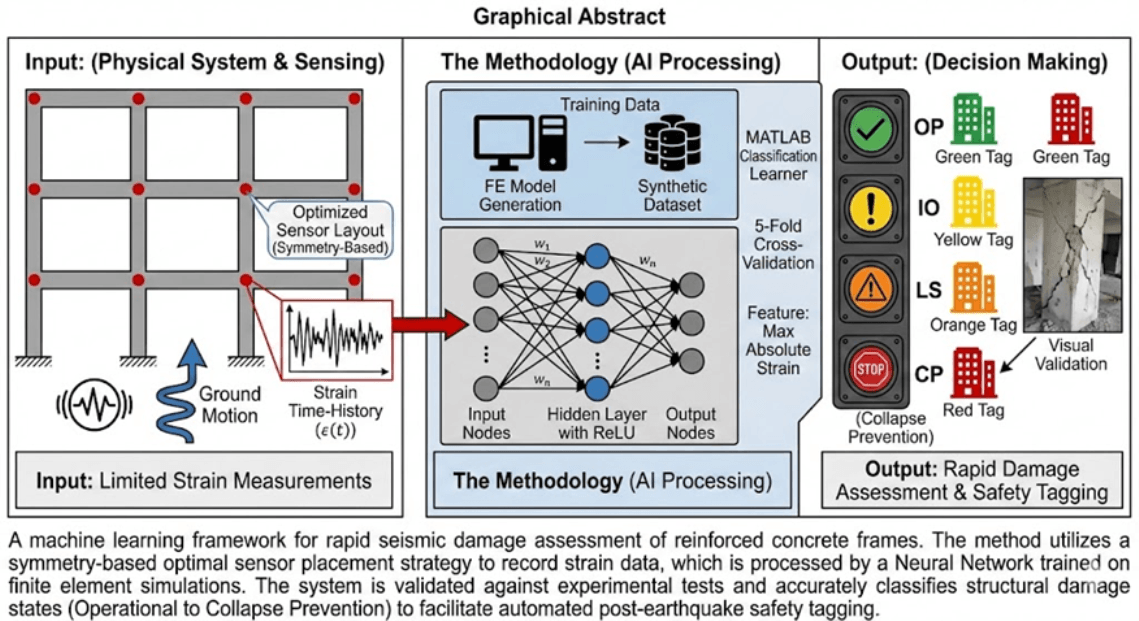
Rapid quantification of seismic-induced damage immediately following an earthquake is critical for determining whether a structure is safe for continued occupation or requires evacuation. This study proposes a novel damage identification method that utilizes limited strain data points, significantly reducing installation, maintenance, and data analysis costs compared to traditional distributed sensor networks. The approach integrates finite element (FE) modeling to generate capacity curves through pushover analysis, incorporates noise-augmented datasets for Artificial Neural Network (ANN) training, and classifies structural conditions into four damage levels: Operational (OP), Immediate Occupancy (IO), Life Safety (LS), and Collapse Prevention (CP). To evaluate the method’s accuracy and efficiency, it was applied to two reinforced concrete (RC) frames; a single-story frame tested experimentally under cyclic loading and a three-story frame analyzed under various lateral load patterns. Strain data from selected beam and column ends were used as ANN inputs, while the corresponding damage classes served as outputs. Confusion matrix results demonstrated high true positive rates (>85% for the single-story and >90% for the three-story frame), even with a reduced number of sensors. The model also exhibited strong robustness to White Gaussian Noise (SNR = 2.5–5 dB) and generalized effectively to nonlinear time-history analyses under scaled ground motions (PGA = 0.1–1.0 g). Feature selection using the MRMR and ANOVA algorithms further enhanced computational efficiency. Overall, the proposed ANN-based framework has strong potential for real-time structural health monitoring applications.Graphic Abstract
Keywords
Earthquakes worldwide continue to inflict devastating damage on buildings and infrastructure, causing human casualties, economic losses, and long-term social disruption [1,2]. Large-magnitude seismic events often lead to partial or complete collapse of buildings, rendering many unoccupiable, with secondary effects such as fires, loss of utilities, and impeded rescue operations. In the aftermath of a strong earthquake, rapidly distinguishing which buildings remain safe to occupy vs. those that need evacuation, repair, or even demolition is crucial to prevent further loss of life and to prioritize emergency response.
Traditionally, this building safety-assessment task has been handled by structural experts conducting visual inspections [3]. Inspectors look for visible damage such as cracks, spalling, deformation, or misalignment. While visual inspection is indispensable, it has several drawbacks: outcomes depend heavily on the skill, experience, and thoroughness of the investigator; assessments are subjective; and the process is very time-consuming, especially over large urban regions or for complex structures.
In order to overcome these limitations, damage intensity level identification can be automated via Structural Health Monitoring (SHM) systems [4]. These systems employ sensors installed on structures before seismic events, to continuously measure responses during or after earthquakes [5]. Often accelerometers are used to record dynamic responses; the time-series acceleration data are converted into the frequency domain (for example, extracting natural frequencies, frequency response functions, or mode shapes) in order to identify damage-sensitive features [6,7]. However, transforming from the time domain into frequency-based representations inevitably involves some loss of information (such as transient or nonstationary features), which may reduce the accuracy or sensitivity of damage detection. Also, measured acceleration magnitude is not directly proportional to damage intensity, as it is influenced by many factors (ground motion amplitude, structural damping, stiffness, soil–structure interaction etc.).
Time-domain measurement and damage detection have potential advantages because it avoids conversion losses; temporal evolution of signals (e.g., in acceleration, strain, velocity, displacement) may retain richer signatures of damage, especially for small or localized damage, or for nonlinear structural behavior. Among sensors usable for time-domain damage detection, strain gauges hold particular promise [8–11]. First, they are in many cases much less expensive than other sensing modalities like dense arrays of accelerometers. This tends to make installation and maintenance cost lower. Second, strain is directly related to deformation and hence more directly indicative of damage intensity, which means measured strain data can potentially be tied more closely to damage severity.
However, using strain data for damage identification has its own challenges. Due to the localized nature of strain, measurements obtained from a single gauge reflect only the deformation at the instrumentation point, potentially limiting the detection of global damage mechanisms distributed elsewhere. For a robust and reliable global damage assessment, many strain gauges might need to be deployed [12]. But increasing the number of sensors increases cost (hardware, installation, maintenance), leads to large quantities of data to store and process, and adds complexity (wiring or wireless telemetry, data synchronization, etc.). Thus, there is a need for an SHM system that can infer global structural condition from limited measured strain data when buildings are subjected to seismic actions.
While strain gauges see broad application in general structural damage identification, their use for seismic-induced damage assessment remains an under-investigated area. Traditional methods for identifying seismic damage typically rely on accelerometer data [13–16], meaning the utility of using limited strain measurements for this purpose has received insufficient attention. To bridge this gap, this study leverages Artificial Neural Networks (ANNs). In the field of SHM, ANNs are a prominent and powerful tool, known for their ability to map the complex, non-linear relationship between various structural response parameters (such as acceleration, frequency, or strain) and the resulting damage characteristics (presence, location, and severity) [17–20]. ANNs can be trained on simulated or experimental data representing both undamaged and various damaged states, enabling them to learn the unique damage patterns or fingerprints in the sensor readings. It is shown in this study that, using strains measured at a limited number of locations, the global response of a reinforced concrete (RC) frame under seismic excitation can be predicted with high accuracy. The proposed approach enables damage intensity estimation in a near-automated manner. The outcome of this study is significant for automated seismic-induced damage identification, offering a viable alternative to resource-intensive traditional inspection, and overcoming the limitations of both frequency-domain based accelerometer methods and purely localized strain-based approaches.
2 Proposed Seismic-Induced Damage Estimation Algorithm
As illustrated in Fig. 1, the proposed algorithm for seismic-induced damage assessment is divided into three main phases. The first phase involves the development of a detailed finite element (FE) model of the structure to obtain its capacity curve. As shown in Fig. 2, the capacity (pushover) curve is a fundamental tool in performance-based seismic engineering, characterizing the global lateral load–deformation response of a structure subjected to monotonically increasing seismic demand. This curve graphically represents the structural capacity in terms of lateral strength and displacement, offering valuable insights into its expected nonlinear behaviour during seismic events. The length and orientation of the inelastic branch (i.e., post-yield region) indicate the structure’s ductility and ability to dissipate energy. Furthermore, specific points along the curve can be associated with global damage thresholds corresponding to widely recognized seismic performance levels, namely Operational (OP), Immediate Occupancy (IO), Life Safety (LS), and Collapse Prevention (CP). The OP level is associated with elastic response, where negligible structural damage is expected. At the IO level, structural response approaches yielding, implying minor damage to primary elements. The LS level denotes moderate damage, in which the structure exceeds its yield capacity but has not yet reached its ultimate strength. Finally, the CP level indicates severe degradation beyond ultimate capacity, where the structure is at imminent risk of collapse. Capacity curves are obtained through nonlinear static pushover analyses performed under various lateral load patterns. Seismic design standards typically recommend at least two lateral loading distributions: one proportional to the first mode shape (often resembling an inverted triangular profile) and another proportional to the floor masses. Additional patterns may be employed for structures exhibiting complex dynamic behaviour such as tall buildings where higher vibration modes significantly influence the response [21].
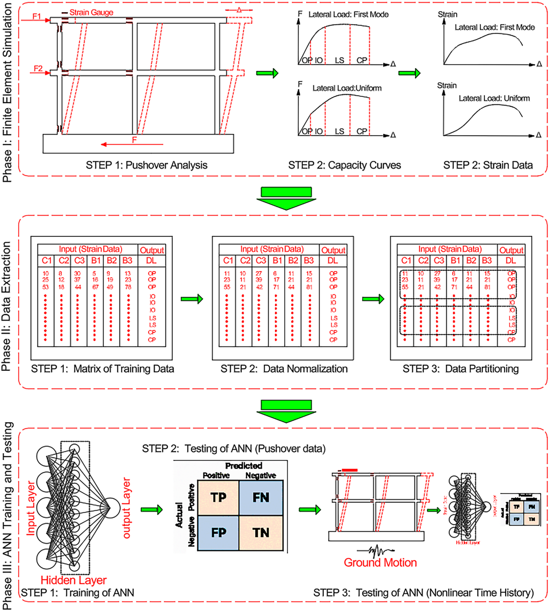
Figure 1: Flowchart of the seismic-induced damage estimation algorithm. Note: C1–C3 represent the measured strains in the columns (1st to 3rd story), B1–B3 represent the measured strains in the beams, and DL denotes the structural damage limit states.
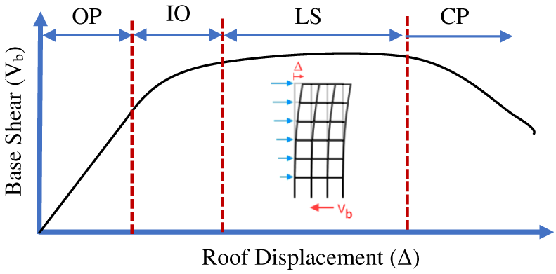
Figure 2: Capacity curve and damage levels of a structure.
Within the proposed automated seismic-induced damage assessment framework, pushover analysis offers several advantages. Most notably, despite yielding relatively accurate inelastic results [22], it eliminates the dependency of the finite element analysis on the selected ground motion characteristics like duration, frequency content, and peak acceleration. Pushover analysis simplifies the analysis and considerably reduces computational effort relative to time-intensive nonlinear time-history (NTH) simulations. In the proposed algorithm, when pushover analysis is being conducted, strain data at critical structural locations should be recorded. These locations generally coincide with regions of large bending moment demand, commonly found near the ends of beams and columns. In multi-story and multi-span structural systems, these critical regions can be efficiently identified by locating plastic hinges that reach their ultimate capacities earlier than others during pushover analysis.
The second phase involves preparing the training and testing datasets for a neural network classifier. As depicted in Fig. 1, the strain values at the identified critical locations serve as input parameters, while the corresponding damage state constitutes the output of the neural network. Damage states can be derived from the capacity curve and categorized into the four designated performance levels of OP, IO, LS, and CP (see Fig. 2). In addition, building damage states can be also identified by monitoring formation of plastic hinges in the structural elements. Because the data obtained from numerical simulations are inherently noise-free, white Gaussian noise with varying intensities should be injected into the dataset to simulate potential measurement uncertainties and enhance model robustness. Subsequently, the dataset is partitioned to prevent overfitting, and to improve generalization performance.
The third and final phase focuses on evaluating the performance of the trained neural network. Model accuracy and classification reliability can be assessed using several established techniques, including confusion matrix analysis. To further validate the model’s generalizability, the trained network that has used pushover analysis data set is subjected to results derived from NTH analyses using multiple ground motions. This step ensures that the classifier can accurately identify damage levels when presented with previously unseen input data. It is important to emphasize that the trained Neural Network is inherently structure-specific. Since the correlation between local plastic strain and global damage limits relies on the unique stiffness distribution, material properties, and geometry of the frame, the ANN cannot be directly transferred to a different structure (e.g., one with a different number of stories or bay widths) without retraining. The proposed workflow dictates that for every new building to be monitored, a corresponding baseline Finite Element model must be created to generate a bespoke training dataset, ensuring that the network is calibrated to the specific dynamic characteristics of that asset.
The following sections present and discuss results from two representative case studies to demonstrate the effectiveness of the proposed methodology. The first case study considers a single-story, single-bay reinforced concrete (RC) frame tested under cyclic loading. The second case study investigates a numerically modelled three-story, three-bay RC frame.
The first investigated structure, shown in Fig. 3, is a one-bay single-story RC frame which was detailed according to special moment frame requirements in ACI 318-14 [23]. Its columns (200 mm × 200 mm) and beams (250 mm × 200 mm) were transversely reinforced with 8 mm diameter hoops spaced at 40 mm near column ends and 50 mm near beam ends, both closer than code-specified maximums (50 and 55 mm, respectively). Outside critical regions, hoop spacing was 80 mm, satisfying ACI 318-14 [23] limits (less than six times the smallest longitudinal bar diameter). Beam–column joints were provided with transverse reinforcement similar to the column confinement, and the column hoops were extended 200 mm into the foundation to ensure anchorage. Column longitudinal bars were lap-spliced at mid-height with a length of 800 mm, complying with ACI 318-14 [23] splice requirements. Overall, the frame detailing ensures compliance with strong column–weak beam design, adequate confinement, joint reinforcement, and proper splicing, representing a ductile special moment frame configuration. The 8-, 12-, and 16-mm diameter bars used to reinforce the frame have a yield strength of 532, 444, and 537 MPa, and their ultimate strengths are 693, 565, and 681 MPa. The compressive strength of concrete on standard cylinder was 30 MPa. The experimental testing was conducted in two stages. First, a constant vertical load was applied to the top of each column to simulate gravity loads. Next, a lateral quasi-static cyclic load was applied to the frame, following the displacement-controlled protocol specified in FEMA 461 [24]. The hysteretic behavior of the frame was captured by recording the applied lateral force and the corresponding lateral displacement at the height of the beam centerline. In addition, strains at both ends of left column and the left end of the beam (see Fig. 3a) were recorded at different drift levels. More detail about the tested frame and its quasi-static cyclic test results can be found in [25].
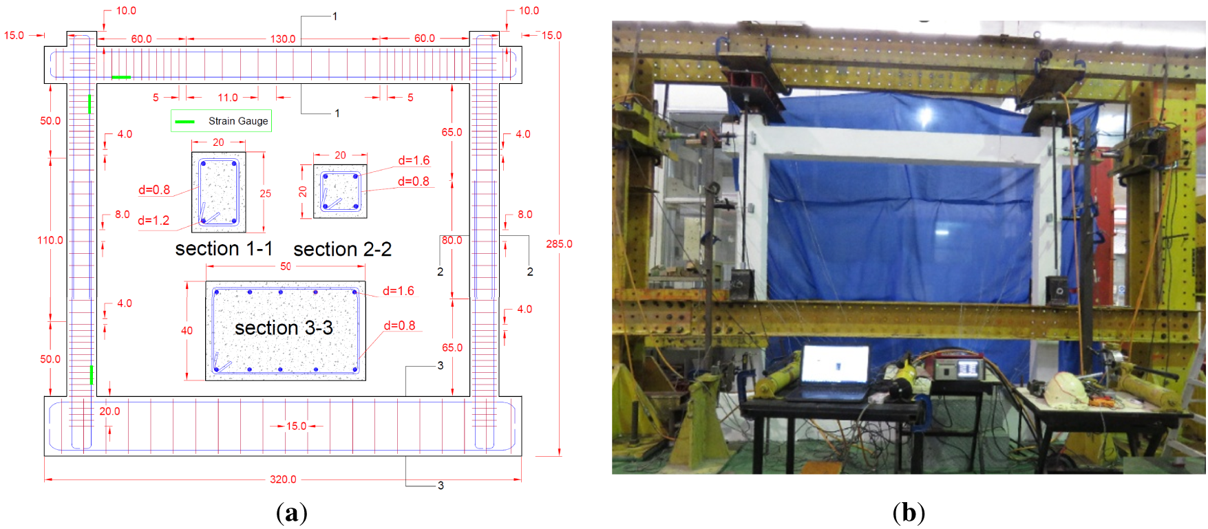
Figure 3: The tested RC frame (a) reinforcement detail (b) test [27].
As illustrated in Fig. 4, the second structure is a three-story, three-bay reinforced concrete frame. It features consistent span lengths and a floor height of 3 m. The frame was designed to withstand both gravity and seismic actions in accordance with Eurocode 8 [26] requirements. The applied dead and live loads were 5 and 2 kN/m2, respectively. It was assumed that the frame is situated on very stiff soil (Eurocode 8, Type A) with a peak ground acceleration of 0.3 g. Spectrum Type 2 and a behavior factor (q) of 1.5 were utilized for the seismic force calculations. As shown in Fig. 4, the cross-sectional dimensions for the frame’s columns are 0.4 m × 0.4 m at the ground level, 0.4 m × 0.35 m at the first level, and 0.35 m × 0.35 m at the roof level. All beams across every floor have a rectangular cross-section of 0.4 m ×0.3 m. The reinforcement ratio in the columns ranges from 2.0% at the ground level to 1.3% at the roof level. For the beams, the ratio varies from 0.89% at the ground floor to 0.4% at the roof level. The longitudinal reinforcing bars used in both columns and beams possess yield and ultimate strengths of 537 and 681 MPa, respectively. The shear links have corresponding yield and ultimate strengths of 532 and 693 MPa.
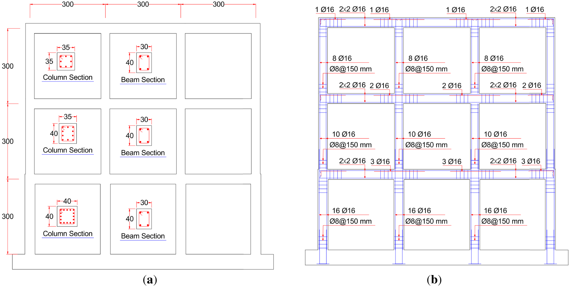
Figure 4: Details of the investigated 3-story RC frame (a) cross-sectional dimensions of beams and columns (b) reinforcement detailing.
Finite element (FE) simulation of reinforced concrete structures employs various modeling methods to capture their complex nonlinear behavior under load. The primary approaches include lumped plasticity, fiber models, and continuum models. Lumped plasticity simplifies nonlinearity by concentrating inelastic behavior into zero-length rotational springs at member ends (e.g., beam-column interfaces). Its advantage lies in its computational efficiency and ease of implementation, but it has the disadvantage of only being able to capture overall member response and not the spread of yielding along the member [28]. Fiber models divide the cross-section into longitudinal fibers (representing concrete and steel reinforcement) where a uniaxial stress-strain law is applied to each fiber, integrating them to get sectional forces and stiffnesses. This approach offers a good balance between computational speed and the ability to capture the spreading of plasticity, but it is typically limited to modeling flexural-dominant behavior. Continuum models (often using solid elements or layered shell elements) represent the concrete and steel as separate materials throughout the volume, relying on constitutive models (like damage or plasticity) to describe the material response, including complex phenomena like cracking and crushing. The major advantage of continuum models is their accuracy and generality in capturing localized failure modes (e.g., shear and bond-slip), but they are highly demanding computationally and require careful mesh design and specialized material calibration.
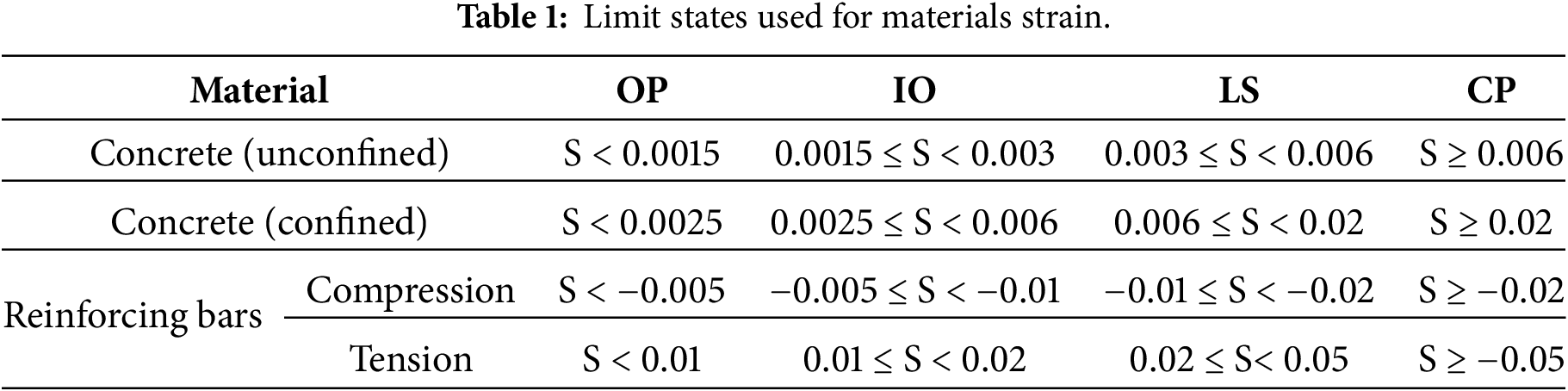
In this study, the FE models of both structures were established using SAP2000 software [29]. This software primarily models material nonlinearity in frame elements using the concept of plastic hinges. Two main methods are available for defining these hinges for reinforced concrete (RC) analysis: concentrated plasticity (simplified) and distributed plasticity (fiber-based). The concentrated plasticity method uses predefined or code-based force-deformation or moment-rotation curves assigned to discrete zero-length hinges located at the member ends. The distributed plasticity method uses fiber hinges (P-M2-M3 interaction). As illustrated in Fig. 5, the software discretizes the cross-section for each hinge into several small areas, or fibers, which represent either concrete or reinforcement steel. During the analysis, the program applies a specific stress-strain material model to each fiber (e.g., Mander’s model for confined concrete, bilinear model for steel). It then integrates the forces and stiffnesses of all fibers across the section to calculate the overall axial force and bending moments and their corresponding deformations. In this study, fiber hinges were employed and assigned to both ends of the frame’s beams and columns. The stress-strain relationships employed for concrete and reinforcing bars are shown in Fig. 6. Furthermore, Table 1 displays the assigned limit states for damage class of each material. The limit states defined in Table 1 establish the thresholds for the formation of plastic hinges in the numerical model. It is important to note that for a cross-section to be classified into a specific damage state (OP, IO, LS, or CP), it is not necessary for both the concrete and steel strain limits to be met simultaneously. The damage state is governed by the ‘worst-case’ condition; if either the concrete compressive strain or the steel tensile/compressive strain exceeds the specified limit, the section is assigned to that damage level. The strain limits presented in Table 1 were adopted from standard constitutive models (e.g., Mander’s model for concrete) and standard code limits (such as ACI 318-14 [23] for unconfined concrete strain).
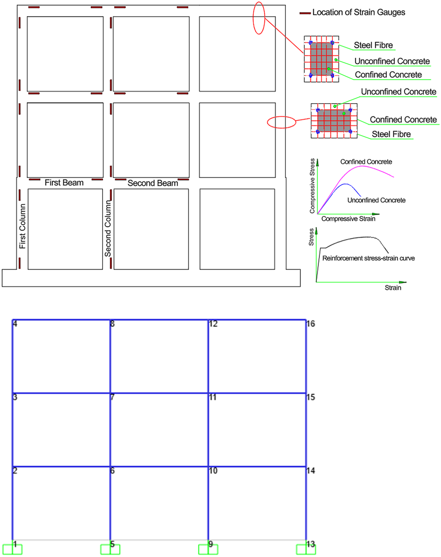
Figure 5: Selected 3-story reinforced concrete column and its finite element model.
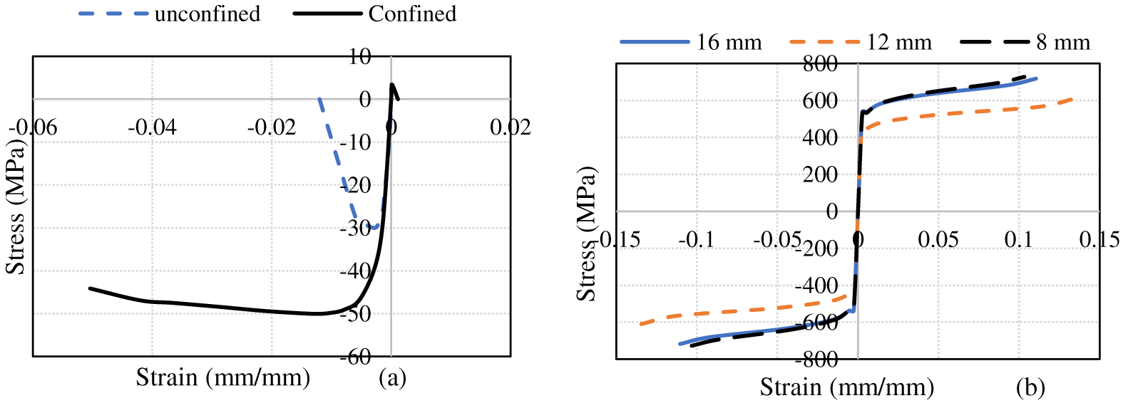
Figure 6: Strain-stress relationships employed for materials (a) concrete (b) reinforcing bar.
In both the single-story verification model and the three-story application frame, the ground-level column bases were modeled as fully fixed supports, restraining all translational and rotational degrees of freedom. The structural components were simulated using nonlinear frame elements in SAP2000, where inelastic behavior was captured through a fiber-based lumped plasticity approach by assigning plastic hinges at the element ends. Since the nonlinear deformation is concentrated at these discrete hinge locations rather than distributed across a continuum mesh, the numerical solution is inherently independent of element discretization; consequently, a traditional mesh sensitivity analysis was not required [28,30,31]. The numerical model followed a strict two-phase loading protocol. First, a constant vertical load was applied as point loads to the top of each column to establish the initial gravity loads, identically mirroring the experiment. Only after these axial loads were fully applied and the structure reached equilibrium was the lateral displacement-controlled load introduced at the beam end. In contrast, for the three-story frame representing a realistic building scenario, gravity loads were applied as distributed loads along the beam spans, and lateral seismic demands followed the specific modal and triangular load patterns detailed in Section 7.
5 Validation of Finite Element Models
Before proceeding with the generation of training datasets, the reliability of the Finite Element (FE) modeling approach was rigorously validated against experimental data. It is important to note that while the physical single-story frame was tested under quasi-static cyclic loading to capture its hysteretic behavior, the proposed damage assessment algorithm utilizes nonlinear static (pushover) analysis to generate capacity curves. To validate the FE model for this purpose, the backbone (envelope) curve was extracted from the experimental cyclic response. This backbone curve represents the structure’s force-displacement capacity under monotonic demand and serves as the benchmark for validation. Consequently, the validation process involved comparing this experimental backbone against the monotonic pushover curve produced by the FE simulation. This comparison confirms that the simplified pushover model accurately captures the global stiffness, ultimate strength, and deformation limits necessary for the neural network training, without the need for computationally intensive cyclic simulations for every data point.
As shown in Fig. 7a, the backbone curve derived from the single-story frame’s cyclic response was particularly well-captured by the FE model, although the experimental data for comparison ceased at approximately a 4% drift ratio, limiting validation beyond that point. Furthermore, as demonstrated by Fig. 7b,c, the FE model also adequately predicted the strains measured at critical locations, specifically the left end of the frame beam and the base of the left column. While the FE model slightly underestimated the strain values at these two locations for a drift ratio less than 1.5%, a close agreement was observed between the experimental and FE strain data within the 1.5% to 3% drift range. Despite minor discrepancies, the overall accuracy of the FE model is considered sufficient to support the subsequent investigation.
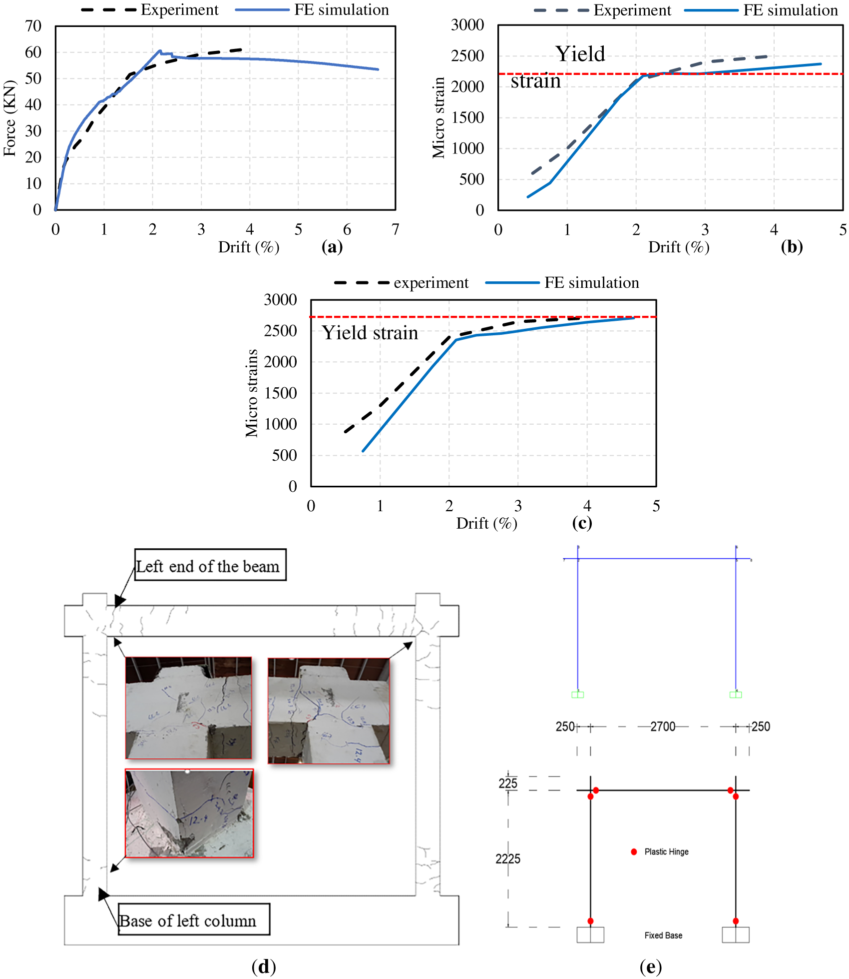
Figure 7: Comparison between finite element and experiment results of single-story frame (a) capacity curves (b) strain measured at the left end of beam (c) strain measured at the base of left column (d) observed damage to the single-story frame [27] (e) established FE model and location of plastic hinges.
To validate the model’s ability to capture the correct failure mechanisms, a comparison was made between the numerically predicted plasticity and the physically observed damage. Fig. 7d presents the experimental state of the frame at the conclusion of the test, highlighting severe concrete cracking and spalling concentrated at the beam ends and the column base. While the lumped plasticity modeling approach (Fig. 7e) does not simulate discrete crack propagation, the damage distribution is effectively captured by monitoring the strain evolution in the assigned plastic hinges. As shown in the strain-drift histories of Fig. 7b,c, the FE simulation predicts that the reinforcement at the beam ends and column base exceeds the yield strain threshold at approximately 2% drift, with strains accumulating significantly as the drift increases to 4.5%. This numerical confirmation of extensive yielding corresponds directly to the regions of severe physical damage observed in the experiment, confirming that the FE model accurately reproduces the structure’s critical failure modes.
It is acknowledged that the use of nonlinear static (pushover) analysis represents a simplification of the true dynamic behavior of the structure. Because this method neglects dynamic effects such as damping forces, inertial effects, and hysteretic energy dissipation under cyclic reversals, the strain values obtained may differ slightly from those recorded under dynamic earthquake loading. However, a primary objective of this study is to demonstrate that the proposed ANN framework is sufficiently robust to yield accurate damage predictions despite these simplifications. The results presented in subsequent sections confirm that this simplified approach provides a highly reliable basis for rapid damage classification, effectively balancing computational efficiency with predictive accuracy.
6 Application of the Proposed Damage Estimation Algorithm on the Single-Story RC Frame
The proposed seismic-induced damage estimation algorithm was initially applied to the single-story reinforced concrete frame. The training dataset was established using results from the finite element model, while the experimentally obtained data was used to test the trained neural network. As illustrated in Fig. 3a, three locations were strategically selected for strain data recording and subsequent training of the neural networks: both ends of the left column and the left end of the beam. These locations were chosen because they are expected to experience high bending moments. Table 2 displays four different combinations of strain data examined for training and testing the neural networks: Case 1 included data from all three locations; Case 2 utilized only the strains obtained from the left column; Case 3 considered the strain at the base of the left column and the left end of the beam; and Case 4 combined the strain data from the top end of the left column with the strain data from the left end of the beam. A total of 484 datasets were generated from the conducted pushover analysis, and these were employed for the training and validation of the neural networks. In addition, 11 sets of strain data obtained from the experiment at the same locations were used to test the trained neural networks against unseen datasets. To generate the training datasets, the finite element (FE) model was subjected to incremental lateral displacements. Strain values were recorded at critical locations, specifically the beam and column ends, at each loading increment. As illustrated in Fig. 8, the resulting datasets capture the full spectrum of the frame’s structural behavior, spanning from the elastic range to inelastic response at a 6.6% drift ratio.
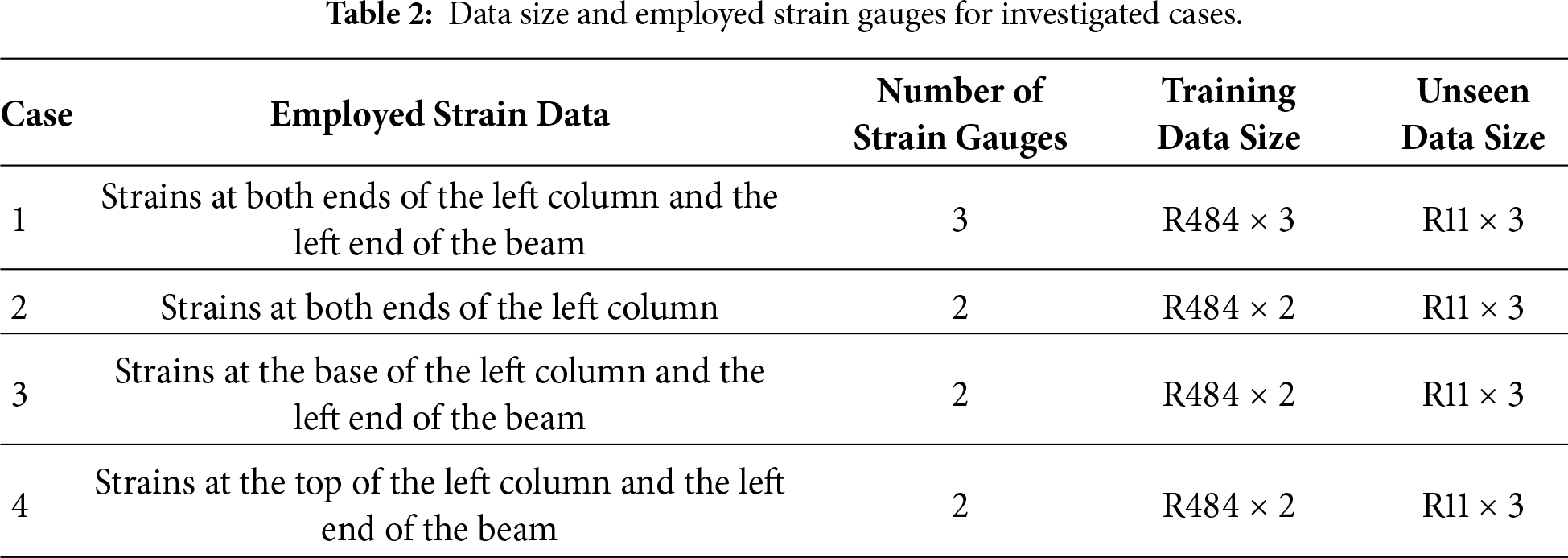
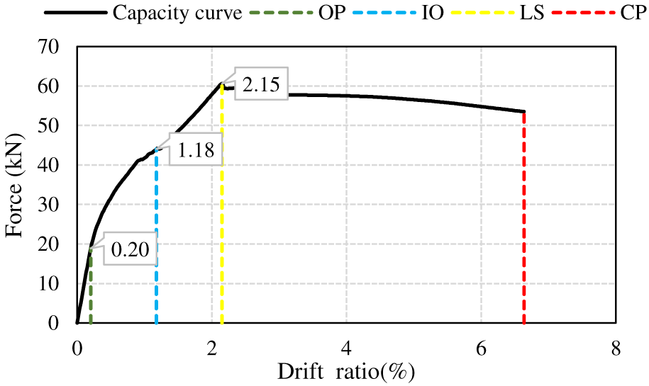
Figure 8: Considered damage classes for the single-story RC frame.
Four distinct damage classes were considered for the frame: (1) Operational (OP), (2) Immediate Occupancy (IO), (3) Life Safety (LS), and (4) Collapse Prevention (CP). As shown in Fig. 8, the OP damage class corresponds to a drift ratio less than 0.2%, where the frame exhibits an elastic response. The IO damage class represents a drift ratio between 0.2% and 1.18%, during which slight damage was observed in the beams and columns in the physical experiment [25]. The LS damage class corresponds to a drift ratio between 1.18% and 2.15%, where significant cracking and the yielding of reinforcing bars were detected. Finally, the CP damage class represents a drift ratio exceeding 2.15%, characterized by larger cracks and concrete spalling reported during the test. It is important to emphasize that the specific inter-story drift limits used to define the damage classes for this single-story frame (i.e., 0.2%, 1.18%, and 2.15%) were derived directly from the experimental damage observations recorded for this specific test specimen (i.e., reference [25]). These values serve as a validated benchmark for this particular study. However, for general applications to other structural systems, these limit states are not fixed constants. Instead, they must be determined individually for each structure through nonlinear static (pushover) analysis. By monitoring the sequence and severity of plastic hinge formation in the beam and column elements during the pushover analysis, the global drift ratios corresponding to the transitions between operational, immediate occupancy, life safety, and collapse prevention performance levels can be explicitly identified from the structure’s unique capacity curve.
To ensure the reproducibility and robustness of the neural network model, the classification model was developed using the MATLAB Classification Learner Toolbox [32] employing a 5-fold cross-validation scheme. This validation strategy involved randomly partitioning the dataset into five equal disjoint subsamples (folds); for each of the five iterations, four folds were utilized for training while the remaining fold served as the validation set. This ensures that every data point is used for both training and validation, providing a more reliable estimate of the model’s generalization error compared to a simple holdout split. Prior to training, the input predictors were manually normalized using Min-Max scaling to map the strain data to the range [–1, 1], thereby eliminating scale bias and facilitating stable convergence. The network architecture utilizes a fully connected feedforward topology, employing the ReLU (Rectified Linear Unit) activation function in the hidden layers for efficient non-linear mapping, and a Softmax function in the output layer to generate probabilistic classifications for the damage states. The training process involved minimizing the Cross-Entropy loss function, with the final model performance reported as the average accuracy across all five validation folds. The optimal number of neurons in the hidden layer was determined through a trial-and-error method as suggested in literature [33]; after several trials, the number was set to 10, as this configuration yielded the best performance for the trained networks.
Single-Story Frame Results and Discussions
The confusion matrix was employed to evaluate the effectiveness of the proposed algorithm in predicting the damage classes of the frames. In machine learning, particularly in classification tasks, the confusion matrix is a fundamental performance evaluation tool. It provides a tabular summary comparing the predicted class labels against the actual (true) class labels of a dataset. Figs. 9–12 present the confusion matrices obtained for the four different sets of input parameters investigated.
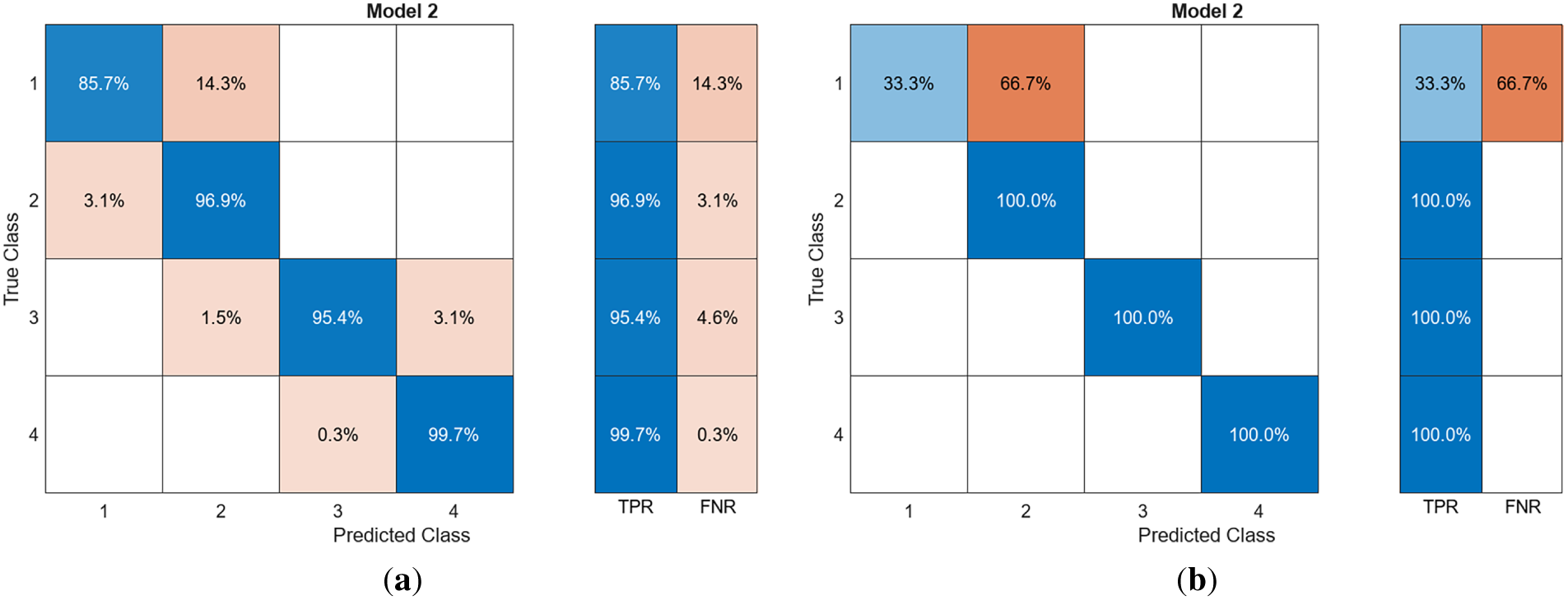
Figure 9: Confusion matrices obtained for Case 1 (a) FE model data (b) experimental data.
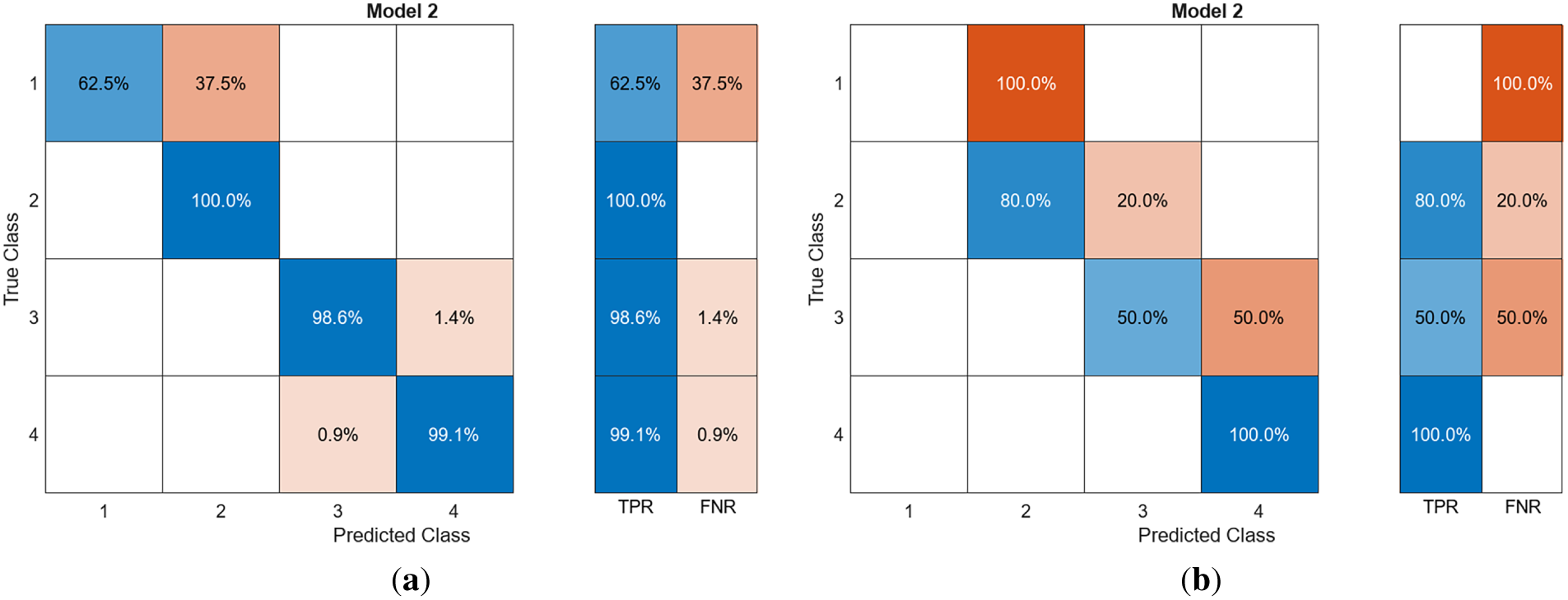
Figure 10: Confusion matrices obtained for Case 2 (a) FE model data (b) experimental data.
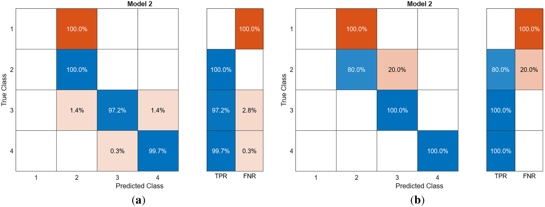
Figure 11: Confusion matrices obtained for Case 3 (a) FE model data (b) experimental data.
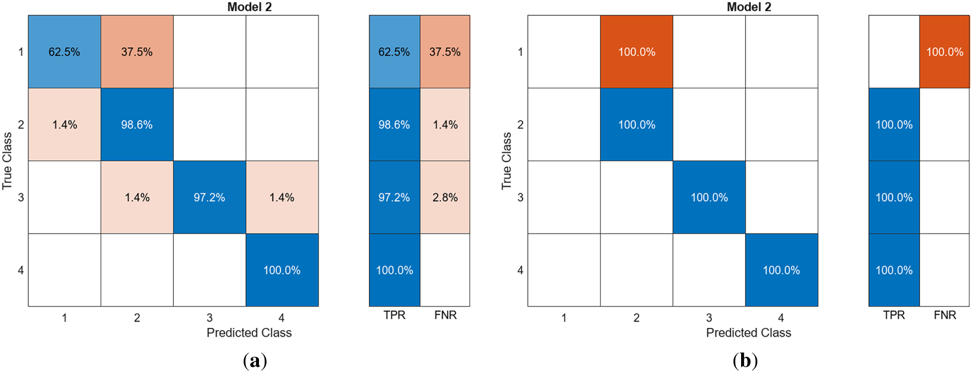
Figure 12: Confusion matrices obtained for Case 4 (a) FE model data (b) experimental data.
Case 1 (Fig. 9) represents the most comprehensive dataset, utilizing strain measurements from both ends of the left column and the left end of the beam (three strain gauges in total). The network achieved high prediction accuracy, with True Positive Rates (TPR) exceeding 85% across all four damage classes. The False Negative Rates (FNR) were below 5% for most classes, indicating strong model reliability. The TPR is the proportion of correctly classified observations per true class, while the FNR shows the proportion of incorrectly classified observations per true class. The only noticeable misclassification occurred for the OP damage class, which was occasionally predicted as IO. This discrepancy can be attributed to the FE model’s underestimation of strain at low drift ratios (below 1.5%), as shown previously in Fig. 7. Despite this minor deviation, the model accurately identified all other damage classes for both training and unseen test datasets, confirming the robustness of the strain-based approach.
When the number of strain measurements was reduced to two, as in Cases 2–4 (Figs. 10–12), the neural network still demonstrated remarkable predictive capability. However, a gradual reduction in accuracy was observed, particularly for the lower damage class (OP), where the sensitivity to strain variations is minimal. Case 2, which used strains from both ends of the left column, captured axial and flexural effects in the column but lacked sufficient information about beam deformations, leading to slightly lower accuracy compared to Case 1. Case 3, using strain data from the column base and the left beam end, achieved relatively better accuracy due to the inclusion of both vertical and horizontal deformation responses. Similarly, Case 4, which used strain data from the column top and left beam end, maintained strong classification performance, demonstrating that strain readings near potential hinge regions are particularly informative for damage prediction. In summary, the single-story frame results demonstrate that the proposed damage estimation algorithm can accurately and reliably predict multiple damage classes using a small number of strain measurements for the investigated frame. While the results demonstrated the framework’s robustness by successfully testing an ANN trained on idealized numerical data against a physical experimental specimen, thereby implicitly accounting for material inhomogeneity and construction tolerances, further steps are required for field deployment. Future research should explicitly investigate the system’s sensitivity to sensor malfunction. To mitigate the risk of a single sensor failure compromising the prediction, future iterations of the model should incorporate sensor redundancy and be trained using ‘data dropout’ techniques, where random sensor inputs are intentionally nullified during training to force the network to learn alternative correlation paths.
7 Application of the Proposed Damage Estimation Algorithm on the Three-Story RC Frame
The three-story RC frame shown in Fig. 4 was subjected to pushover analysis using four different lateral load patterns. These load patterns included a mass-proportional distribution and patterns derived from the first three mode shapes of the frame. As illustrated in Figs. 13–15, each lateral load pattern produced distinct capacity spectra, failure modes, and consequently, different strain distributions at the critical locations of beams and columns.
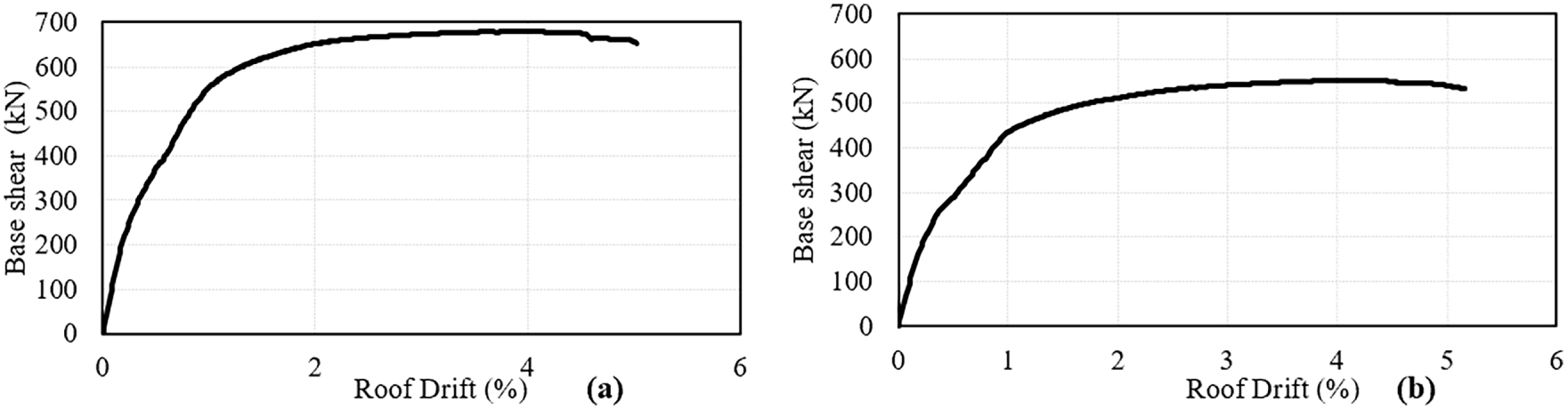
Figure 13: Capacity curves obtained from pushover analysis, plotting base shear (kN) vs. roof drift ratio (%) (a) mass proportional lateral load (b) first mode proportional lateral load.
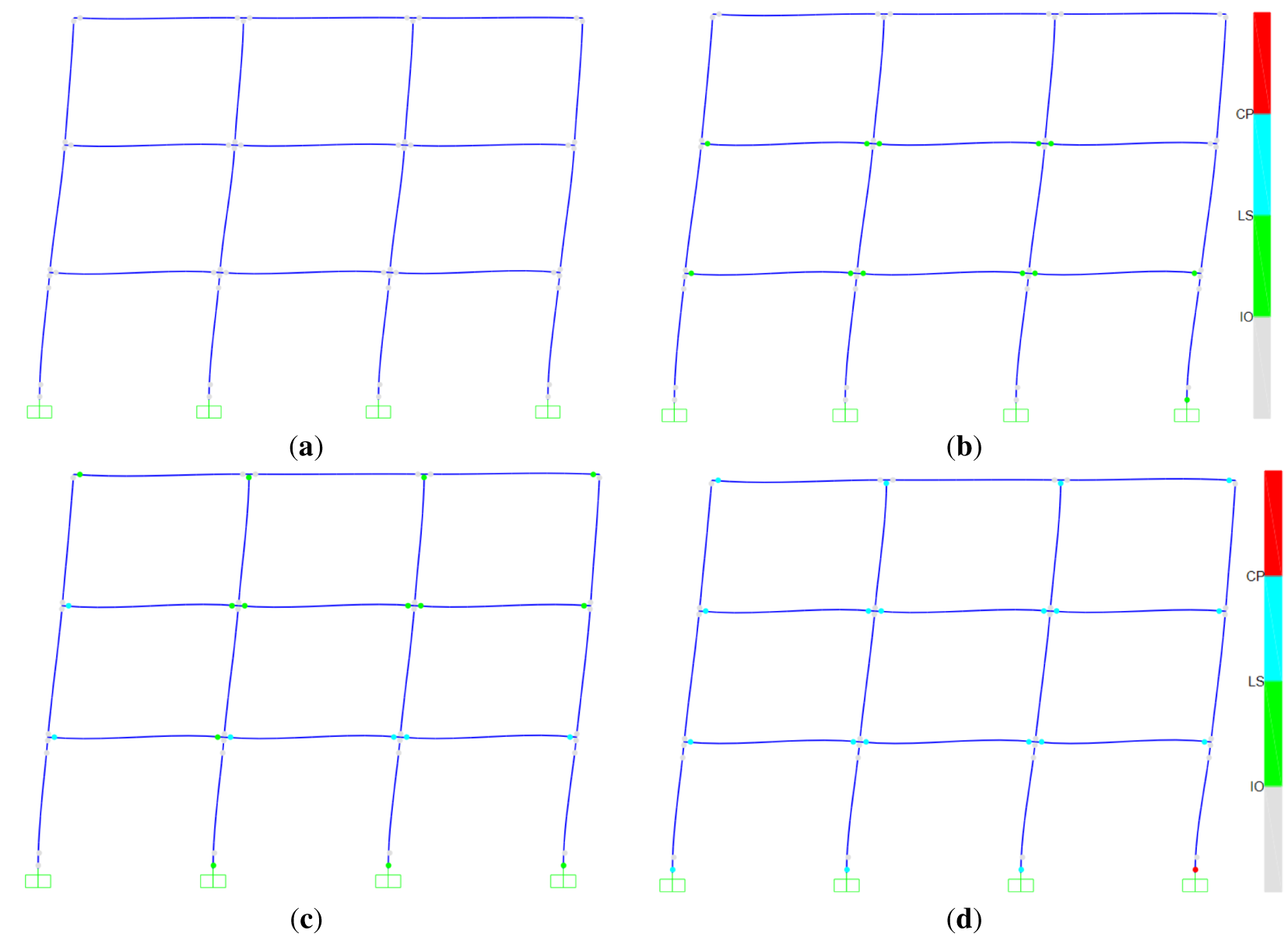
Figure 14: Development and progression of plastic hinges in the 3-story frame at varying roof drift ratios when a mass-proportional lateral load pattern was used (a) 1% (b) 2% (c) 3% (d) 5%.
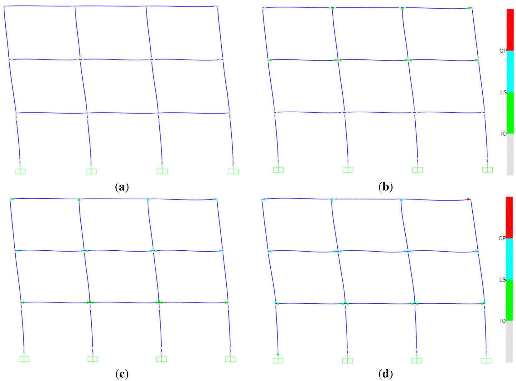
Figure 15: Development and progression of plastic hinges in the 3-story frame at varying roof drift ratios when the lateral load pattern followed the first mode shape (a) 1% (b) 2% (c) 3% (d) 5%.
As shown in Fig. 5, the strains recorded at both ends of the first- and second-span beams and columns were selected for further analysis. The selection of sensor locations for the three-story frame was driven by the capacity design principles inherent to seismic-resistant structures. In moment-resisting frames, nonlinear behavior and damage accumulation are anticipated to concentrate in specific ‘plastic hinge’ zones, typically at the ends of beams and the base of ground-floor columns, while the rest of the structure remains largely elastic. Consequently, strain gauges were strategically positioned within these critical regions to capture the maximum deformation demands. Furthermore, to optimize the sensor network without compromising data quality, the instrumentation plan exploited the geometric and structural symmetry of the frame. As the three-bay frame is symmetric in terms of geometry, material properties, and gravity loading, the seismic response of the outer bays is expected to be mirrored. Therefore, sensors were installed only at the beam ends and column locations of the first and second spans. The response of the third span is effectively captured by the symmetry of the first span, rendering additional sensors in that bay redundant for the purpose of global damage classification. This reduction minimizes the computational input dimension while ensuring that the Neural Network receives a complete representation of the frame’s critical damage mechanisms.
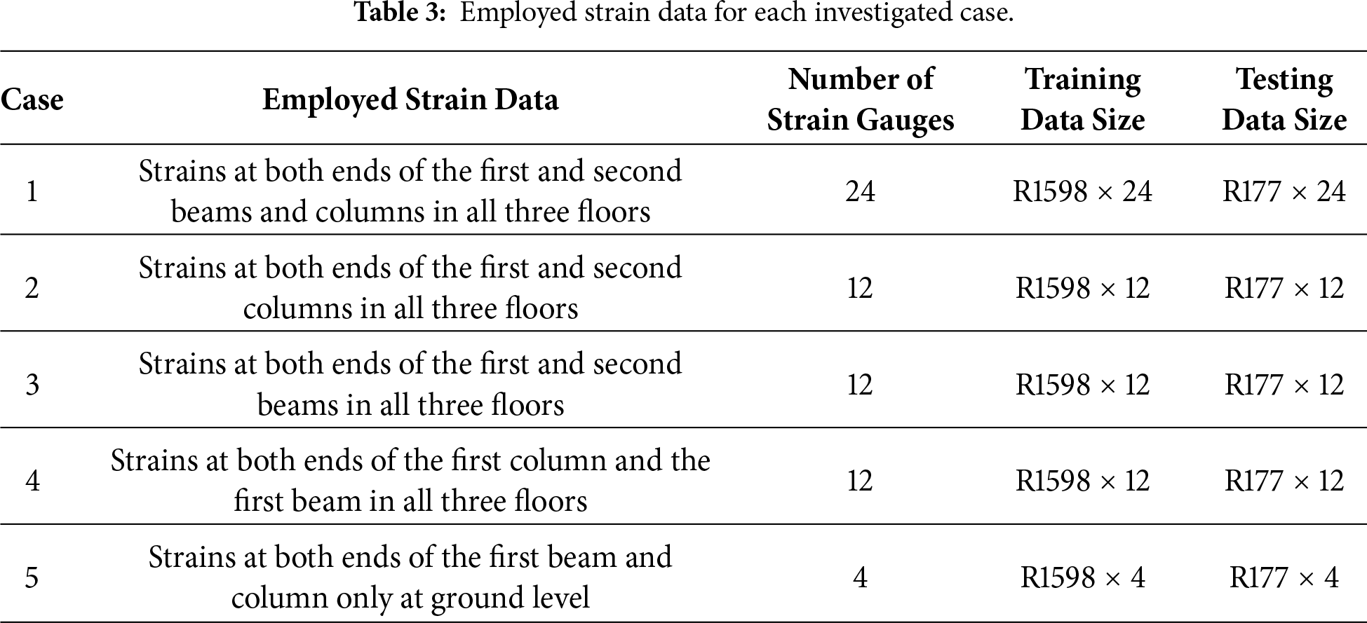
Five different combinations of strain data were examined. These five combinations of strain data enabled an element-wise and location-wise evaluation of how strain measurements influence damage classification accuracy. Similar to the single-story frame, four damage classes (OP to CP) were considered for the three-story frame. However, unlike the single-story frame where damage classes were defined based on inter-story drift ratios, the classification for the three-story frame was defined according to the formation of plastic hinges in beams and columns. This approach was adopted because the pushover analyses with different lateral load patterns resulted in varying damage mechanisms at different drift ratios. As presented in Table 3, pushover analysis produced 1775 strain data points per measurement location. Approximately 10% of this dataset was used to test the trained neural network for unseen data. The architecture and hyperparameters of the trained neural network were identical to those employed for the single-story frame.
7.1 3-Story Frame Results and Discussions
Figs. 16–20 illustrates the confusion matrices obtained for the five investigated cases that were presented in Table 3. The results collectively demonstrate the robustness and generalization capability of the proposed neural network model in classifying damage states of the 3-story reinforced concrete (RC) frame.
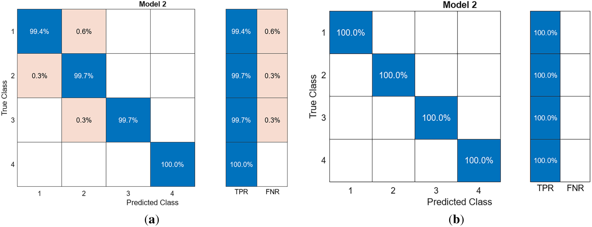
Figure 16: Confusion matrices obtained for Case 1 (a) validation (b) test.
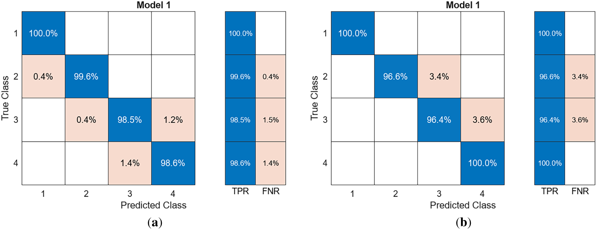
Figure 17: Confusion matrices obtained for Case 2 (a) validation (b) test.
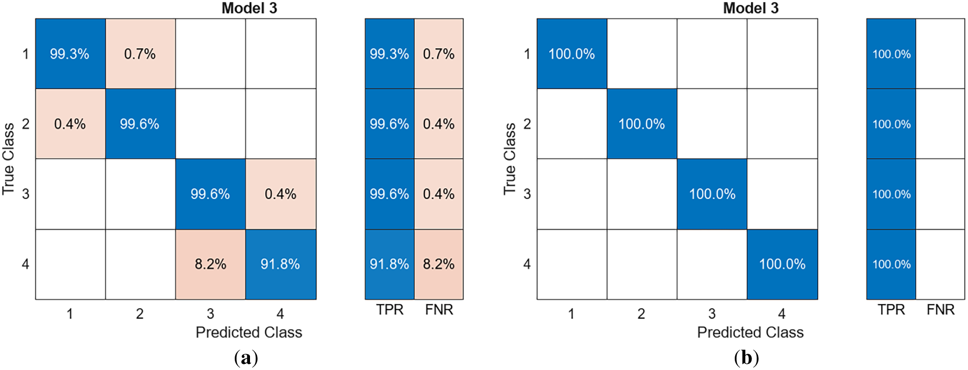
Figure 18: Confusion matrices obtained for Case 3 (a) validation (b) test.
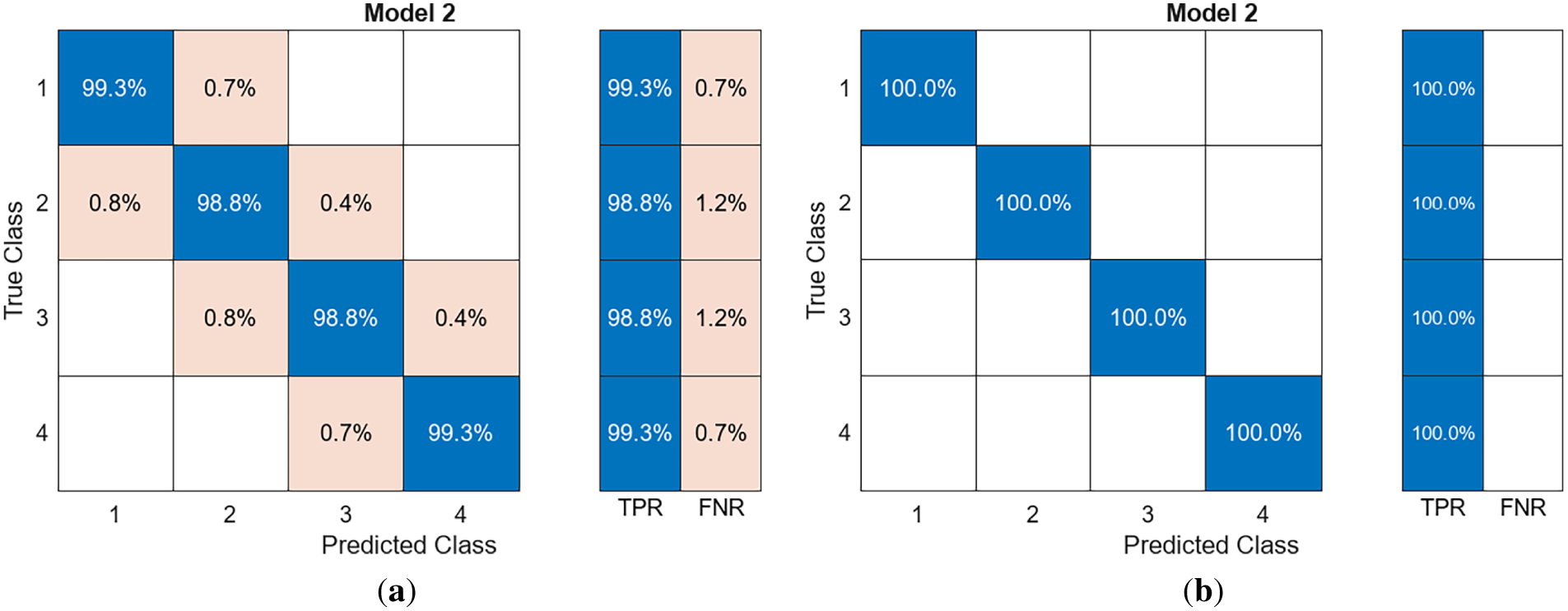
Figure 19: Confusion matrices obtained for Case 4 (a) validation (b) test.
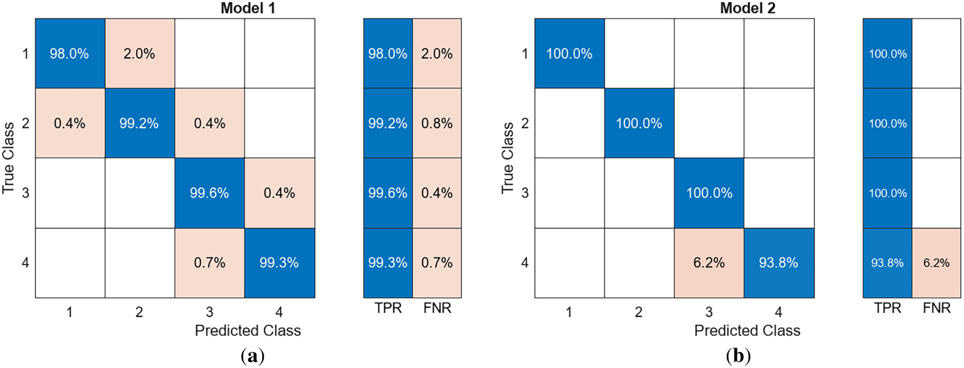
Figure 20: Confusion matrices obtained for Case 5 (a) validation (b) test.
Across all five investigated cases, the TPR exceeded 90% for all four damage classes, confirming the high predictive accuracy of the model. This outcome highlights the strong correlation between the measured strain data and the global damage state of the structure. The model’s ability to generalize was further verified through testing with 10% unseen data, where excellent performance was maintained across all damage classes.
Case 1 (Fig. 16), which utilized strain data from all 24 measurement locations (both ends of the first and second beams and columns at all three stories), achieved outstanding classification accuracy. Notably, a perfect 100% TPR was obtained for both training and test datasets across all four damage classes. This result establishes a benchmark, showing that a comprehensive representation of the structural strain field enables near-perfect identification of the frame’s damage state. In Case 2 (Fig. 17), which used only 12 strain measurements from the columns, the overall classification accuracy remained above 90%, though minor misclassifications appeared in the lower damage classes. This suggests that while column strains capture significant aspects of global response, they may not fully reflect beam flexural contributions that influence early-stage (OP and IO) damage identification.
Conversely, Case 3 (Fig. 18), which used strain data only from beams, achieved a prediction accuracy comparable to Case 1, with 100% TPR recorded in the test phase. This indicates that beam strains are highly sensitive to global deformations and damage progression, likely because flexural behaviour in beams governs the formation of plastic hinges in moment-resisting frames. Case 4 (Fig. 19) examined a reduced dataset of 12 strain locations from both ends of the first beam and first column at all floors. Despite having half the number of strain data points compared to Case 1, the prediction accuracy remained essentially unaffected. Both training and test datasets achieved TPR values close to or equal to 100%, indicating that strain measurements at strategically chosen locations can provide sufficient information to characterize the overall frame damage state.
Remarkably, Case 5 (Fig. 20), which used only four strain measurement points (both ends of the first beam and first column at the ground floor), also yielded near-perfect classification accuracy. The results demonstrate that strain responses at critical beam–column locations on the ground floor are strongly correlated with the global structural behaviour and can effectively represent the system’s overall damage condition. This finding suggests that a minimal instrumentation scheme, if properly positioned, can be used to accurately assess structural damage using machine learning techniques.
7.2 Effect of Noise on Predictions
To evaluate the robustness of the trained neural network against measurement uncertainties, White Gaussian Noise (WGN) was added to the strain input data. Figs. 21–23 present the confusion matrices obtained for three representative cases (Case 1, Case 3, and Case 5) after the inclusion of noise at two signal-to-noise ratios (SNRs): 2.5 and 5 dB. The predictions obtained from the noisy datasets were compared with the baseline results from the noise-free data (Figs. 16, 18 and 20).
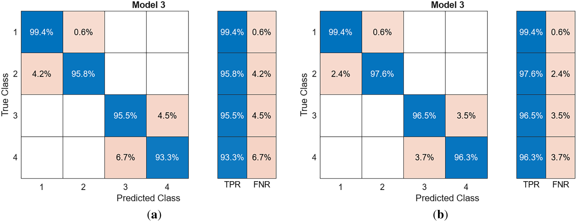
Figure 21: Confusion matrices obtained for Case 1 when data was contaminated with White Gaussian noise (a) SNR = 2.5 dB (b) SNR = 5 dB.
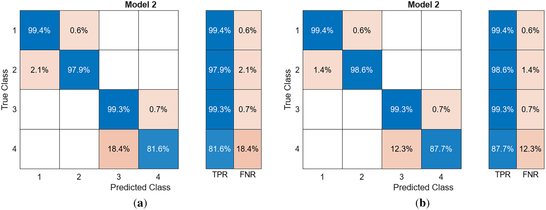
Figure 22: Confusion matrices obtained for Case 3 when data was contaminated with White Gaussian noise (a) SNR = 2.5 dB (b) SNR = 5 dB.
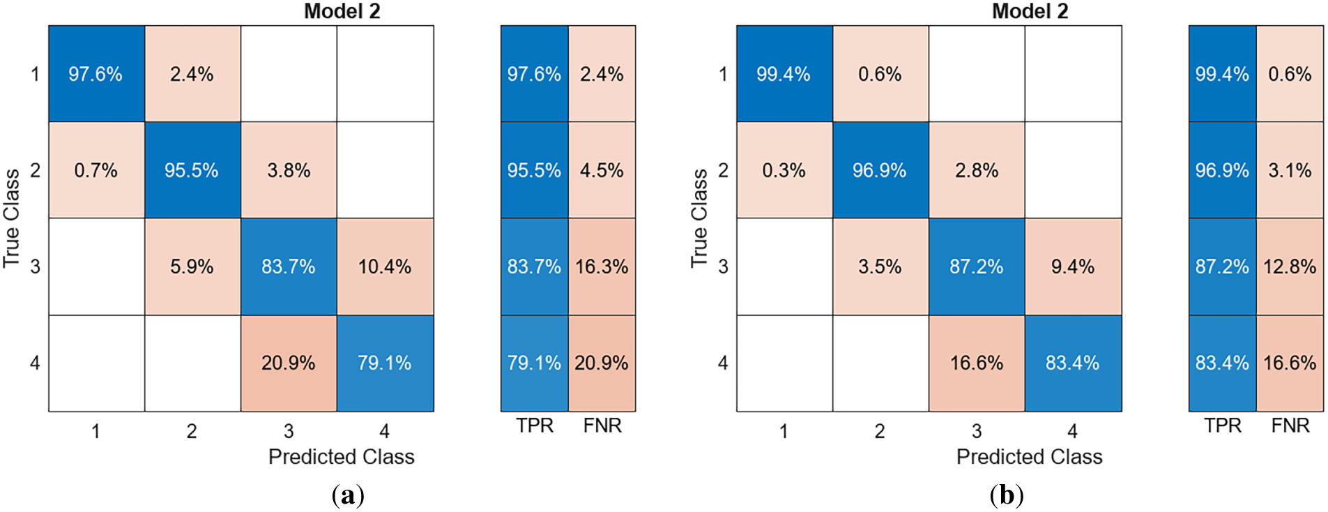
Figure 23: Confusion matrices obtained for Case 5 when data was contaminated with White Gaussian noise (a) SNR = 2.5 dB (b) SNR = 5 dB.
The results demonstrate that the neural network maintains a high level of predictive performance even when the input strain data are contaminated by noise. However, a gradual degradation in classification accuracy is observed as the noise level increases, particularly at the lower SNR (2.5 dB). In Case 1, which used the full set of 24 strain measurement locations (Fig. 21), the trained network exhibited excellent noise tolerance. When subjected to 5 dB noise, the TPR remained close to those of the noise-free condition, with minimal misclassification across all four damage classes. Even at the more severe 2.5 dB noise level, the overall classification accuracy remained above 90%, indicating that the network had successfully learned robust structural features that were not overly sensitive to perturbations in strain data. This suggests that data redundancy from multiple sensors enhances the model’s resilience to measurement errors.
In Case 3, which employed only 12 strain inputs from beam ends (Fig. 22), the effect of noise became slightly more pronounced. While the overall accuracy under 5 dB noise remained high (above 85%), noticeable confusion appeared between adjacent damage classes, especially between OP and IO. At 2.5 dB noise, the misclassification rate increased marginally, reflecting that when the number of strain inputs is reduced, the model becomes more susceptible to distortion in the input signal. Nevertheless, the network still maintained acceptable predictive capability, confirming that its learning process generalized well beyond idealized (noise-free) conditions.
The most significant test of robustness occurred in Case 5 (Fig. 23), where only four strain measurement locations were used, representing the most data-sparse configuration. Despite this limitation, the network continued to perform strongly. Under 5 dB noise, the confusion matrix showed minimal degradation, with correct classification rates exceeding 90% across all classes. Even at 2.5 dB noise, while a few OP samples were misclassified as IO, the higher damage states (LS and CP) remained perfectly identified. This indicates that the neural network learned hierarchical features that distinguish between small and large strain responses, making it inherently robust to random fluctuations in input data.
While this study validated the robustness of the ANN against White Gaussian Noise, which simulates standard electrical interference and measurement floor noise, it is acknowledged that field applications face broader sources of uncertainty. Specifically, issues such as sensor malfunction or data loss present a significant challenge. To mitigate this, future research should investigate ‘sensor dropout’ training techniques, where the network is trained with randomly omitted inputs to develop redundancy, ensuring that the classification remains stable even if individual sensors fail. Furthermore, regarding long-term sensor drift and environmental thermal effects, practical implementation would require established compensation protocols. Since seismic damage is primarily driven by dynamic excursions, the influence of long-term drift can be effectively minimized by re-zeroing the strain baseline immediately prior to a seismic event or by utilizing temperature-compensating strain gauges, ensuring that the network processes only the relevant earthquake-induced demand.
7.3 Damage Class Predictions under Ground Motion Excitations
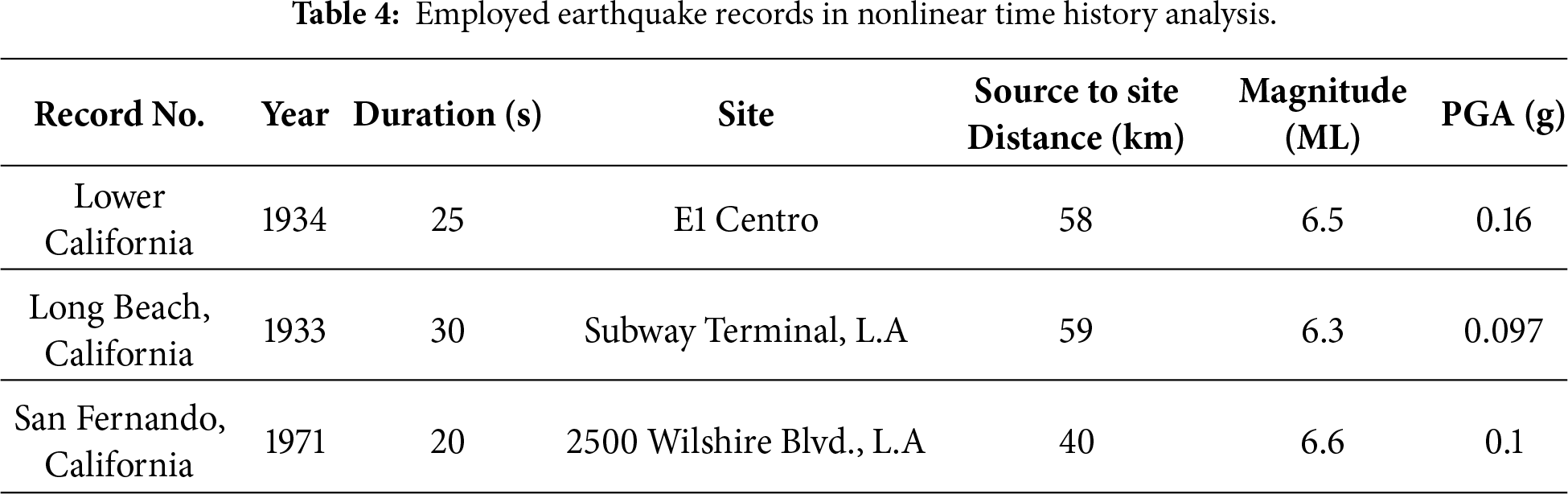
To evaluate the accuracy and robustness of the proposed seismic-induced damage estimation algorithm under real earthquake excitations, the three-story frame was subjected to three different ground motion records, and its damage classes were predicted using the trained neural network. Before conducting nonlinear time history analyses, the Peak Ground Accelerations (PGA) of the selected records were scaled to 0.1, 0.5, and 1.0 g to represent minor, moderate, and strong earthquake intensities, respectively. The characteristics of the selected earthquake records are summarized in Table 4. During each analysis, strain time histories were recorded at 24 locations as illustrated in Fig. 5, resulting in 1913 strain data points per measurement location. To account for environmental effects, the strain data were contaminated with white Gaussian noise corresponding to a signal-to-noise ratio (SNR) of 2.5 dB.
To determine the optimal combination of strain measurement locations, two feature selection algorithms, Minimum Redundancy Maximum Relevance (MRMR) [34] and Analysis of Variance (ANOVA) [35], were employed. Both are filter-based methods commonly used in machine learning for dimensionality reduction. MRMR selects features that maximize their relevance to the target variable while minimizing redundancy among them, using mutual information as the selection criterion. This approach effectively balances feature diversity and informativeness, particularly for high-dimensional datasets, although it can be computationally demanding and less reliable for small samples. In contrast, ANOVA evaluates each feature independently by comparing between-class and within-class variance to identify features that significantly discriminate between target categories. ANOVA is simple, fast, and interpretable, but it assumes data normality and homogeneity of variance, and it does not account for feature interdependencies or nonlinear effects.
Figs. 24a and 25a illustrate the first 12 features identified by the MRMR and ANOVA algorithms, respectively. In both figures, columns 1–8 correspond to strain data from the ground floor, columns 9–16 to the first floor, and columns 17–24 to the roof level. Within each floor, the first four columns represent strains recorded at both ends of the first two columns, while the next four columns correspond to strains measured at both ends of the two beams. As shown in Fig. 24a, the MRMR algorithm predominantly selected features from the ground floor (7 out of 12), with only two features from the roof. Conversely, the ANOVA algorithm distributed the selected features more evenly across the three floors (4 per floor). In both cases, most selected features corresponded to beam strains rather than column strains, which is consistent with previous findings and reflects the dominant role of beams in contributing to the lateral stiffness of moment-resisting frames.
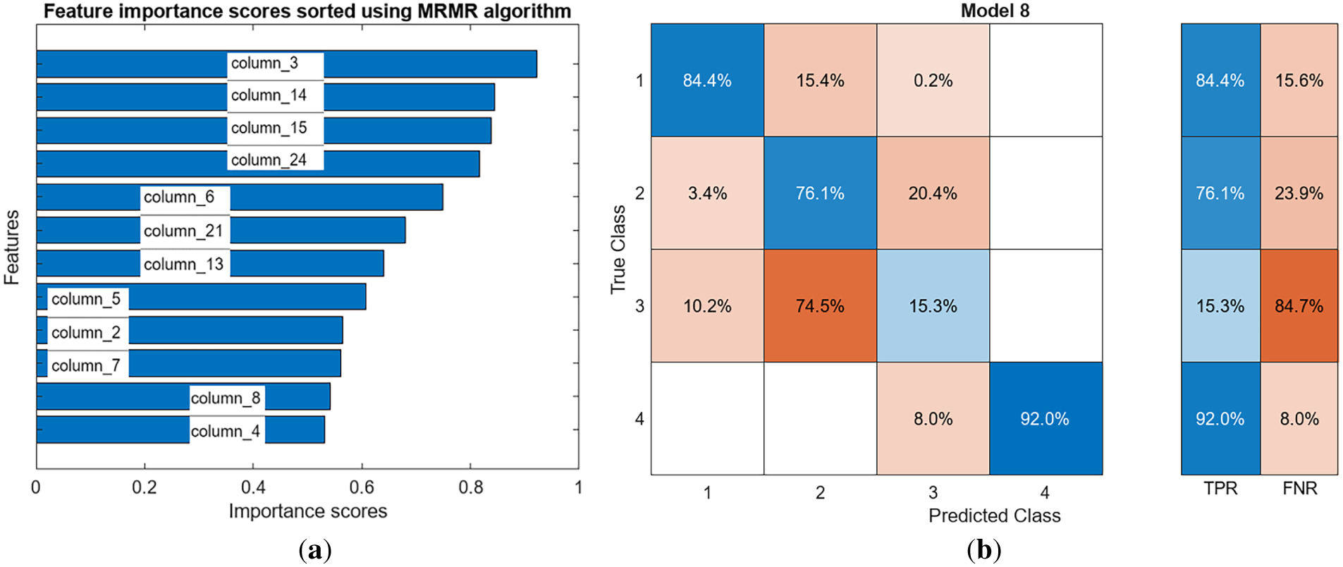
Figure 24: (a) MRMR algorithm’s first 12 features (b) confusion matrix based on nonlinear time history analysis.
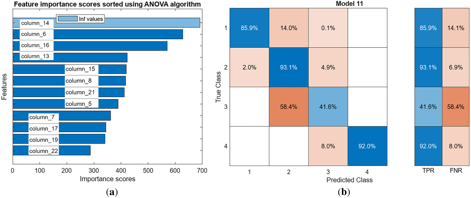
Figure 25: (a) ANOVA algorithm’s first 12 features (b) confusion matrix based on 12 features.
Figs. 24b and 25b show the confusion matrices obtained when the features selected by the two algorithms were used to predict damage classes under nonlinear time history loading. In both cases, the TPR for the first and fourth damage classes exceeded 80%, indicating excellent predictive performance. However, the ANOVA-based feature set yielded a significantly higher TPR for the second damage class compared with the MRMR-based set (93% vs. 76%). Despite this improvement, both algorithms showed lower accuracy for the third damage class, which was frequently misclassified as the second. This misclassification can be attributed to the inherent limitation of the conventional pushover analysis (CPA) used to prepare the training data set. As the reinforced concrete (RC) structure yields, its stiffness degrades, causing the fundamental period to lengthen. This action continuously alters the distribution of inertia forces during an earthquake. Because CPA employs a constant load pattern throughout the analysis, it cannot accurately simulate this continuous force redistribution in the inelastic range. Adaptive Pushover Analysis (APA) [36], however, was specifically developed to address this problem of inertia force redistribution and can thus be used to mitigate this issue.
To further examine the effect of the number of input strain data on prediction accuracy, the number of features selected by the ANOVA algorithm was reduced to eight and six. The resulting confusion matrices are shown in Figs. 26 and 27. When eight strain data points were used, the TPRs for damage classes one, two, and four improved slightly; however, the TPR for the third damage class dropped markedly from 41.6% to 15.3%. This reduction occurred because only one strain measurement from the roof level was retained among the first eight features, whereas, as shown in Fig. 15d, damage may concentrate near the roof. This observation is further supported by Fig. 27, where the exclusion of roof-level strain data (when only six features were used) resulted in a pronounced decrease in the TPR for the third and fourth damage classes. Despite the lower accuracy for the third class, the neural network trained with only six strain gauges still achieved good predictive performance for the other three damage classes.
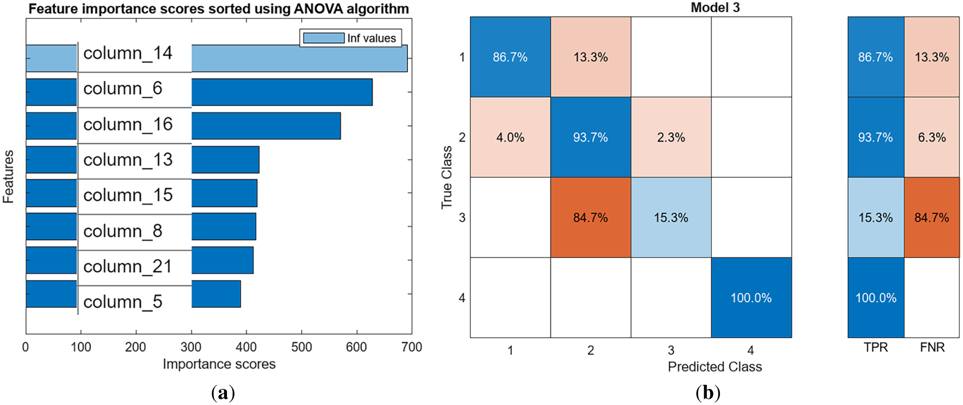
Figure 26: (a) ANOVA algorithm’s first eight features (b) confusion matrix based on eight features.
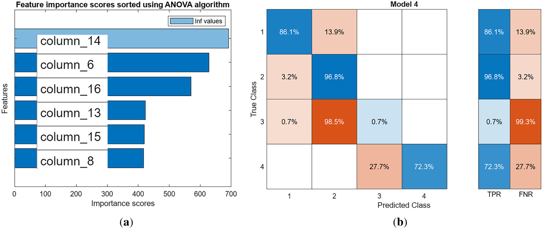
Figure 27: (a) ANOVA algorithm’s first six features (b) confusion matrix based on six features.
The feature selection analysis explained above revealed a significant dependency on upper-floor strain measurements, particularly when distinguishing between transitional damage classes (e.g., IO to LS). This sensitivity aligns with the physical behavior of moment-resisting frames during progressive yielding. As the primary plastic hinges form in the lower-story beams (characteristic of the IO state), the lateral stiffness of the first story decreases, causing a redistribution of seismic demand to the upper stories. Consequently, the strain evolution in the second and third-floor elements acts as a critical indicator for the onset of the Life Safety (LS) limit state. This confirms that the Neural Network is not merely memorizing local data points but is successfully capturing the global force redistribution mechanisms inherent to the structure’s inelastic response.
7.4 Model Understanding and Interpretability
The variation in classification accuracy across the sensor configurations employed for the single-story frame offers valuable insight into the physical behavior driving the neural network’s predictions. The reduced accuracy observed in Case 2, which relied exclusively on column strains, highlights the limitations of monitoring structural elements designed to remain elastic for extended periods. Given that the frame was detailed according to the “strong column-weak beam” design philosophy, the onset of damage, marking the transition from operational to immediate occupancy, is physically initiated by yielding in the beam elements. Consequently, configurations incorporating beam strain data (Cases 1, 3, and 4) provided the network with direct evidence of the developing failure mechanism, resulting in superior classification performance. This confirms that the neural network is not merely fitting data patterns but is effectively identifying the mechanical “hotspots” where seismic energy dissipation and damage concentration occur.
Similarly, the feature selection results provide significant physical insight into the learning process of the model for the three-story frame, bridging the gap between data-driven classification and structural mechanics. As shown in Figs. 24 and 25, both algorithms predominantly prioritized beam strains over column strains. This preference aligns with the “strong column-weak beam” philosophy employed in the frame’s design, where plastic hinges, and thus the primary indicators of energy dissipation and damage, are intended to form in the beams first. Furthermore, the high importance scores assigned to ground-floor sensors (particularly by the MRMR algorithm) reflect the concentration of seismic demand and inter-story drift at the structure’s base. By identifying these physically significant regions as the most relevant features, the neural network effectively “learned” to monitor the locations most representative of global ductility demand. This physical correlation explains the success of sparse sensor configurations (such as Case 5); the model does not require data from every element because the strain state at critical plastic hinge regions serves as a reliable proxy for global structural health.
This study successfully demonstrates an ANN-based algorithm for seismic-induced damage estimation in RC frames using limited strain data, achieving high classification accuracy across OP, IO, LS, and CP damage classes. Beyond theoretical validation, the proposed framework offers significant practical contributions to earthquake engineering and community resilience. First, it facilitates automated post-earthquake tagging by translating global damage state classifications into immediate safety decisions (e.g., Green/Yellow/Red tags), thereby accelerating re-occupancy and minimizing community downtime. Second, the validation of a minimal instrumentation scheme significantly lowers the economic barrier for structural health monitoring, rendering scalable deployment across extensive infrastructure portfolios economically feasible. Finally, the method supports data-driven retrofit prioritization, allowing asset managers to transition from schedule-based to condition-based maintenance by identifying structures entering transitional damage states (e.g., IO to LS) for targeted early intervention, thus optimizing limited retrofitting budgets.
For the single-story frame, predictions aligned well with experimental data, with minimal misclassifications even when using only two strain gauges. The three-story frame results further confirmed the method’s efficacy, maintaining >90% accuracy with as few as four sensors, highlighting the informativeness of strains at beam-column joints. Noise tolerance and performance under dynamic ground motions underscore the model’s robustness, while feature selection algorithms like ANOVA optimized input efficiency, though revealing challenges in distinguishing transitional damage states (e.g., IO-LS). While the proposed ANN-based framework achieves high classification accuracy, limitations of this approach include its reliance on idealized finite element models for training data and its inability to provide explicit analytical expressions (closed-form equations) for damage quantification, which are traditionally preferred in engineering practice for manual verification. The latter limitation is mitigated by two factors. First, the application of feature selection algorithms (MRMR and ANOVA) provides interpretability, ensuring that the model relies on physically significant features, such as beam strains in strong-column/weak-beam frames, rather than arbitrary data patterns. Second, the primary utility of this method lies in automated structural health monitoring systems, where the ANN operates as a real-time computational engine, effectively bypassing the need for manual analytical calculations.
Future work could involve experimental validation on diverse structures and real-time implementation in SHM systems. Furthermore, subsequent research should explore reliability assessments to rigorously quantify the probability of correct damage classification under varying uncertainties, as well as optimization-oriented studies to determine the ideal sensor layouts that maximize classification accuracy while minimizing instrumentation costs. Finally, while this study validated the framework using structures in an initially undamaged state, the methodology is applicable to in-service structures through the use of model updating. Future research should investigate the accuracy of the system when applied to structures with pre-existing damage by calibrating the training stage FE models to reflect prior loading histories.
Acknowledgement: The authors would like to acknowledge the Ministry of Higher Education of Malaysia and Universiti Teknologi Malaysia for the provided financial support.
Funding Statement: This research was funded by UTM Fundamental Research Grant (PY/2024/01221, Cost centre no.: Q.J130000.3822.23H73) and HiCoE Grant Scheme (Cost centre no.: R.J130000.7822.4J738).
Author Contributions: The authors confirm contribution to the paper as follows: conceptualization, Mohammadreza Vafaei; methodology, Mohammadreza Vafaei; software, Abdirahman Abdulkadir; validation, Abdirahman Abdulkadir; formal analysis, Mohammadreza Vafaei; investigation, Mohammadreza Vafaei; resources, Sophia C. Alih; data curation, Abdirahman Abdulkadir; writing—original draft, Mohammadreza Vafaei, Sophia C. Alih; writing—review and editing, Mohammadreza Vafaei, Sophia C. Alih; supervision, Mohammadreza Vafaei; project administration, Sophia C. Alih; funding acquisition, Mohammadreza Vafaei, Sophia C. Alih. All authors reviewed and approved the final version of the manuscript.
Availability of Data and Materials: Data available on request from the authors. The data that support the findings of this study are available from the corresponding author, [Mohammadreza Vafaei], upon reasonable request.
Ethics Approval: Not applicable.
Conflicts of Interest: The authors declare no conflicts of interest.
References
1. Alih SC, Vafaei M. Performance of reinforced concrete buildings and wooden structures during the 2015 Mw 6.0 Sabah earthquake in Malaysia. Eng Fail Anal. 2019;102(6):351–68. doi:10.1016/j.engfailanal.2019.04.056. [Google Scholar] [CrossRef]
2. Ozkula G, Dowell RK, Baser T, Lin JL, Numanoglu OA, Ilhan O, et al. Field reconnaissance and observations from the February 6, 2023, Turkey earthquake sequence. Nat Hazards. 2023;119(1):663–700. doi:10.1007/s11069-023-06143-2. [Google Scholar] [CrossRef]
3. Demir A. Post-earthquake structural damage assessment, lessons learned, and addressing objections following the 2023 Kahramanmaras, Turkey earthquakes. Bull Earthq Eng. 2025;23(3):1107–27. doi:10.1007/s10518-024-02092-8. [Google Scholar] [CrossRef]
4. Gharehbaghi VR, Noroozinejad Farsangi E, Noori M, Yang TY, Li S, Nguyen A, et al. A critical review on structural health monitoring: definitions, methods, and perspectives. Arch Comput Meth Eng. 2022;29(4):2209–35. doi:10.1007/s11831-021-09665-9. [Google Scholar] [CrossRef]
5. Karakostas C, Quaranta G, Chatzi E, Zülfikar AC, Çetindemir O, De Roeck G, et al. Seismic assessment of bridges through structural health monitoring: a state-of-the-art review. Bull Earthq Eng. 2024;22(3):1309–57. doi:10.1007/s10518-023-01819-3. [Google Scholar] [PubMed] [CrossRef]
6. Jamshidi M, El-Badry M. Structural damage severity classification from time-frequency acceleration data using convolutional neural networks. Structures. 2023;54(7):236–53. doi:10.1016/j.istruc.2023.05.009. [Google Scholar] [CrossRef]
7. Cao X, Chen L, Chen J, Li J, Lu W, Liu H, et al. Seismic damage identification of high arch dams based on an unsupervised deep learning approach. Soil Dyn Earthq Eng. 2023;168(12):107834. doi:10.1016/j.soildyn.2023.107834. [Google Scholar] [CrossRef]
8. Zhang J, Guo SL, Wu ZS, Zhang QQ. Structural identification and damage detection through long-gauge strain measurements. Eng Struct. 2015;99(2):173–83. doi:10.1016/j.engstruct.2015.04.024. [Google Scholar] [CrossRef]
9. Li YY. Hypersensitivity of strain-based indicators for structural damage identification: a review. Mech Syst Signal Process. 2010;24(3):653–64. doi:10.1016/j.ymssp.2009.11.002. [Google Scholar] [CrossRef]
10. Rageh A, Linzell DG, Eftekhar Azam S. Automated, strain-based, output-only bridge damage detection. J Civ Struct Health Monit. 2018;8(5):833–46. doi:10.1007/s13349-018-0311-6. [Google Scholar] [CrossRef]
11. Lee JW, Choi KH, Huh YC. Damage detection method for large structures using static and dynamic strain data from distributed fiber optic sensor. Int J Steel Struct. 2010;10(1):91–7. doi:10.1007/BF03249515. [Google Scholar] [CrossRef]
12. Laflamme S, Cao L, Chatzi E, Ubertini F. Damage detection and localization from dense network of strain sensors. Shock Vib. 2016;2016:2562949. doi:10.1155/2016/2562949. [Google Scholar] [CrossRef]
13. Kita A, Cavalagli N, Venanzi I, Ubertini F. A new method for earthquake-induced damage identification in historic masonry towers combining OMA and IDA. Bull Earthq Eng. 2021;19(12):5307–37. doi:10.1007/s10518-021-01167-0. [Google Scholar] [CrossRef]
14. Lu J, Xie Q, Zhu W. Seismic damage detection of ultra-high voltage transformer bushings using output-only acceleration responses. J Civ Struct Health Monit. 2023;13(4):1091–104. doi:10.1007/s13349-023-00695-4. [Google Scholar] [CrossRef]
15. Yagi S, Iyama J, Fukushima Y, Ishida T, Kishiki S, Seike T, et al. Damage detection in ALC exterior walls in steel structural frames subjected to earthquakes using acceleration sensors. J Earthq Eng. 2024;28(4):1109–26. doi:10.1080/13632469.2023.2228928. [Google Scholar] [CrossRef]
16. Lin JF, Li XY, Wang J, Wang LX, Hu XX, Liu JX. Study of building safety monitoring by using cost-effective MEMS accelerometers for rapid after-earthquake assessment with missing data. Sensors. 2021;21(21):7327. doi:10.3390/s21217327. [Google Scholar] [PubMed] [CrossRef]
17. Vafaei M, bin Adnan A, Abd Rahman AB. A neuro-wavelet technique for seismic damage identification of cantilever structures. Struct Infrastruct Eng. 2014;10(12):1666–84. doi:10.1080/15732479.2013.849746. [Google Scholar] [CrossRef]
18. Nick H, Aziminejad A. Vibration-based damage identification in steel girder bridges using artificial neural network under noisy conditions. J Nondestruct Eval. 2021;40(1):15. doi:10.1007/s10921-020-00744-8. [Google Scholar] [CrossRef]
19. Nick H, Ashrafpoor A, Aziminejad A. Damage identification in steel frames using dual-criteria vibration-based damage detection method and artificial neural network. Structures. 2023;51:1833–51. doi:10.1016/j.istruc.2023.03.152. [Google Scholar] [CrossRef]
20. Nick H, Aziminejad A, Hamid Hosseini M, Laknejadi K. Damage identification in steel girder bridges using modal strain energy-based damage index method and artificial neural network. Eng Fail Anal. 2021;119:105010. doi:10.1016/j.engfailanal.2020.105010. [Google Scholar] [CrossRef]
21. Habibi A, Izadpanah M, Namdar Y. A new modal lateral load pattern for improving pushover analysis to estimate nonlinear responses of structures. Aust J Struct Eng. 2022;23(4):289–302. doi:10.1080/13287982.2022.2070112. [Google Scholar] [CrossRef]
22. Jin J, Nagae T, Asai T, Okazaki T, Li J, Lignos DG, et al. Cyclic pushover analysis for seismic response evaluation of a full-scale 10-story steel building tested on the E-Defense shake-table. J Build Eng. 2024;96(3):110552. doi:10.1016/j.jobe.2024.110552. [Google Scholar] [CrossRef]
23. ACI-318. Building code requirements for structural concrete (ACI 318-14) and commentary on building code requirements for structural concrete (ACI 318R-14). Farmington Hills, MI, USA: American Concrete Institute; 2014. [Google Scholar]
24. FEMA 461. Interim testing protocols for structural and nonstructural performance characteristics of determining the seismic components. Redwood City, CA, USA: Federal Emergency Management Agency; 2007. [Google Scholar]
25. Vafaei M, Baniahmadi M, Alih SC. The relative importance of strong column-weak beam design concept in the single-story RC frames. Eng Struct. 2019;185(6):159–70. doi:10.1016/j.engstruct.2019.01.126. [Google Scholar] [CrossRef]
26. EN 1998-1. Eurocode 8: design of structures for earthquake resistance-part 1: general rules, seismic actions and rules for buildings. Brussels, Belgium: European Committee for Standardization; 2004. [Google Scholar]
27. Baniahmadi M, Vafaei M, C Alih S. Cyclic response of reinforced concrete frames partially infilled with relatively weak masonry wall. J Build Eng. 2022;46:103722. doi:10.1016/j.jobe.2021.103722. [Google Scholar] [CrossRef]
28. Vafaei M, Alih SC, Fallah A. The accuracy of the lumped plasticity model for estimating nonlinear behavior of reinforced concrete frames under gradually increasing vertical loads. Struct Concr. 2020;21(1):65–80. doi:10.1002/suco.201800357. [Google Scholar] [CrossRef]
29. SAP2000V-23. Integrated finite element analysis and design of structures basic analysis reference manual. Berkeley, CA, USA: Computers and Structures; 2023. [Google Scholar]
30. López-López A, Tomás A, Sánchez-Olivares G. Influence of adjusted models of plastic hinges in nonlinear behaviour of reinforced concrete buildings. Eng Struct. 2016;124(3):245–57. doi:10.1016/j.engstruct.2016.06.021. [Google Scholar] [CrossRef]
31. Inel M, Ozmen HB. Effects of plastic hinge properties in nonlinear analysis of reinforced concrete buildings. Eng Struct. 2006;28(11):1494–502. doi:10.1016/j.engstruct.2006.01.017. [Google Scholar] [CrossRef]
32. MATLAB version: 9.13.0 (R2022b). Natick, Massachusetts: The MathWorks Inc.; 2022 [cited 2026 Mar 12]. Available from: https://www.mathworks.com/products/new_products/previous_release_overview.html. [Google Scholar]
33. Vafaei M, bin Adnan A, Abd Rahman AB. Real-time seismic damage detection of concrete shear walls using artificial neural networks. J Earthq Eng. 2013;17(1):137–54. doi:10.1080/13632469.2012.713559. [Google Scholar] [CrossRef]
34. Peng H, Long F, Ding C. Feature selection based on mutual information: criteria of max-dependency, max-relevance, and Min-redundancy. IEEE Trans Pattern Anal Mach Intell. 2005;27(8):1226–38. doi:10.1109/TPAMI.2005.159. [Google Scholar] [PubMed] [CrossRef]
35. Connelly LM. Introduction to Analysis of Variance (ANOVA). Med Surg Nursing. 2021;30(3):218. doi:10.62116/msj.2021.30.3.218. [Google Scholar] [CrossRef]
36. Papanikolaou VK, Elnashai AS. Evaluation of conventional and adaptive pushover analysis I: methodology. J Earthq Eng. 2005;9(6):923–41. doi:10.1080/13632460509350572. [Google Scholar] [CrossRef]
Cite This Article
 Copyright © 2026 The Author(s). Published by Tech Science Press.
This work is licensed under a Creative Commons Attribution 4.0 International License , which permits unrestricted use, distribution, and reproduction in any medium, provided the original work is properly cited.
 Downloads
 Citation Tools