Seismic Fragility Evaluation of Elevated Water Storage Tanks Isolated by Optimized Polynomial Friction Pendulum Isolators

1  Introduction

Elevated water storage tanks are designed to store water for both urban areas and industrial facilities. The occurrence of severe ground motions poses a risk of damage to these structures, potentially leading to direct or indirect consequences on public safety. Thus, the secure performance of these structures in severe earthquakes is crucial, ensuring they withstand seismic forces and maintain functionality for vital services like water supply and fire suppression. Several reports have documented incidents following damage to elevated water storage tanks. These include damaging events during past earthquakes, such as the 1960 Chile earthquake, the 1964 Niigata earthquake in Japan, the 1971 San Fernando earthquake, the 1978 Izu Oshima earthquake in Japan, the 1979 Imperial County, California earthquake, and the 1999 Turkey earthquake [1–3], among others. Generally, liquid storage tanks exhibit more complex dynamic behavior during earthquakes than buildings and bridges. This heightened complexity stems from hydrodynamic interactions between the tank and its liquid contents. Considering liquid pressures that arise during an earthquake is significant in the design of structures such as dams and tanks. Several researchers have extensively examined the seismic response of liquid storage tanks. Among recent popular works, Haroun introduced a well-established mechanical lumped-mass model that includes wall flexibility effects [4]. The dynamic behavior of liquid storage tanks under seismic ground motion has been thoroughly studied through numerous analytical and numerical investigations [5]. For a complete bibliographic literature survey on the seismic analysis and design of liquid storage tanks, refer to some review papers recently published [6,7].

Following the 1960 Chile earthquake, seismic analysis of elevated water storage tanks became more critical [8]. These structures also exhibit distinct behavior compared to other structures, resulting in numerous damages over the years. Several approaches exist to mitigate damage to these structures. In general, the implementation of seismic isolators [9] provides a more manageable approach for regulating the transmission of earthquake forces to elevated liquid storage tanks [10]. Base isolation, which involves separating the entire structure from the ground to reduce seismic response, increases the fundamental period of structural vibration and effectively keeps it out of the earthquake’s energetic spectrum [11]. Shrimali and Jangid [12] investigated the seismic response of base-isolated elevated liquid storage tanks by considering two types of isolated tank models, with isolation systems installed at the base and the top of the tower structure. They implemented the mechanical model of lumped masses, known as the sloshing, impulsive, and rigid masses. Shrimali [13] examined the seismic response of elevated liquid storage tanks isolated by the Friction Pendulum System (FPS) under bi-directional excitations. Seleemah and El-Sharkawy [14] studied the seismic response of elevated liquid storage tanks isolated by elastomeric or sliding bearings. Rabiei and Khoshnoudian [15] investigated the seismic response of elevated liquid storage tanks using double-concave FPS with bilinear and trilinear behavior. Moeindarbari et al. [16] examined the multi-level performance of elevated liquid storage tanks isolated with multi-phase FPS under 60 total earthquake records. Paolacci [17] investigated the effectiveness of two isolation systems (i.e., high-damping rubber bearings and the FPS) for the seismic protection of elevated liquid storage tanks. Moslemi and Kianoush [18] studied the applicability of seismic isolation using elastomeric bearings and Lead Rubber Bearing (LRB) (e.g., [19]) for conical elevated liquid storage tanks. The supporting shaft structure was isolated either from the ground or from the vessel mounted on top by isolators. Kumar and Saha [20] examined the seismic performance of elevated liquid storage tanks, considering soil–structure interaction (SSI). The effects of SSI on the peak seismic responses and the seismic fragility of elevated tanks were shown. Ghoohestani et al. [21] analyzed two base isolation systems, an elastomeric bearing and an LRB, to compare their seismic applicability for a conical elevated liquid storage tank subjected to various ground motions. The drilled shaft system was unlinked either from the base or from the top-mounted bowl using the damping devices. Hashemi et al. [22] investigated the effectiveness of seismic isolation using the LRB and FPS for grounded and elevated tanks subjected to bidirectional strong ground motions. They considered two locations for the isolation systems in elevated tanks.

The utilization of sliding bearings for seismic isolation has been validated as a successful technology for safeguarding structures and facilities from seismic events. One type of these isolators is the FPS, characterized by a slider and a concave surface, introduced by Zayas et al. [23] and shown to dissipate energy effectively [24]. Then, in a study conducted by Mokha et al. [25], not only was the effectiveness of the friction pendulum isolator affirmed, but it was also demonstrated that this isolator, characterized by a constant curvature of the surface, maintains a consistent period time, which is a function of the radius of the concave surface. Lu et al. [26] identified the constant period time or frequency in the FPS as a potential drawback. This concern arises when this isolator is subjected to long-period earthquakes, potentially leading to resonance. Researchers have investigated alterations to seismic isolator design, leading to the development of variable-frequency pendulum isolators. Panchal and Jangid [27] conducted a prior study to evaluate slender and broad liquid storage tanks isolated with variable curvature friction pendulum systems (VCFPSs) under near-fault ground motions using a three-degree-of-freedom tank model. They showed that VCFPS isolation effectively reduces base shear, sloshing, and impulsive responses. They [28] also investigated the seismic behavior of liquid storage tanks isolated with Variable Frequency Pendulum Isolators (VFPI) under near-fault, harmonic, and far-field ground motions using a lumped-mass tank model and step-by-step dynamic analysis. Compared with conventional FPS isolation, VFPI systems were found to more effectively reduce base shear and impulsive response, especially under near-fault motions. Pranesh and Sinha [29] observed a positive impact of variable-frequency pendulum isolators with an elliptical surface function on a single-degree-of-freedom (SDOF) isolated structure. The variable-frequency pendulum isolators and their counterparts, such as the Polynomial Friction Pendulum Isolator (PFPI) [30], belong to a general category called the Variable-curvature Friction Pendulum Isolator (VFPI) or Variable-curvature Friction Pendulum Bearing (VFPB) [31–33]. Lu et al. [34] presented comprehensive equations for the restoring force, stiffness, and frequency of VFPI, based on the sixth-order polynomial surface functions. Shaikhzadeh and Karamoddin [35] simulated four VFPIs and one FPS to determine the optimal ranges of the initial isolation period and coefficient of friction, and used them to compare the effectiveness of VFPIs at various Peak Ground Acceleration (PGA) levels for near-fault earthquakes. Zheng et al. [36] developed a superelastic multi-stage VFPI to enhance the seismic resilience of bridges. Krishnamoorthy et al. [37] proposed a new VFPI system to isolate the liquid storage tank subjected to earthquake ground motions. Wei et al. [38] presented a simplified design method for VFPI systems to enable railway bridge bearings to exhibit specific adaptability and self-resetting ability during earthquakes. Lu et al. [39] proposed a systematic design method that allows VFPIs to achieve multiple performance objectives for dual earthquake levels.

Moreover, optimization techniques have been used to craft isolators that achieve the best possible seismic performance. The growing interest in applying optimization methods stems from the vital need for practical, refined seismic design of structures to improve isolator performance. In this context, many researchers have devoted their efforts to exploring the optimal performance of friction-based seismic isolation devices, especially for structures such as buildings and bridges [40,41]. Furthermore, a small number of studies have specifically addressed tanks, as highlighted in the subsequent literature review, focusing on isolators relying on friction. Tsipianitis and Tsompanakis [42] used swarm intelligence optimization algorithms to derive optimal friction coefficients and radii of curvature that enhance the dynamic performance of base-isolated liquid storage tanks. Their focus was on optimizing the sizing of the main parameters for single and triple FPSs. Moreover, Tsipianitis et al. [43] investigated the optimization of single- and triple-FPS systems using various metaheuristic algorithms. Initially, they observed a significant impact of optimizing the parameters of both isolators on the structural response and the acceleration transmitted to the base of the liquid storage tank. Subsequently, a comparison of optimization efficiency revealed consistent patterns across all algorithms.

In addition, although the seismic vulnerability assessment of various structures has been extensively examined in the literature (see, for example, [44–47]), there are limited studies for non-isolated [48] and base-isolated [49,50] ground-supported liquid storage tanks.

Despite extensive research on optimizing seismic isolators for buildings and bridges, no prior study has focused on optimizing the VFPI systems specifically for elevated liquid storage tanks. This omission is significant, given the unique dynamic behavior of these tanks under seismic loading, which demands tailored solutions to mitigate both acceleration and displacement responses. To address this gap, the present study introduces a novel optimization methodology for VFPI systems to enhance their seismic performance. The research emphasizes the critical role of isolator geometry in controlling acceleration and displacement during long-period ground motions. By optimizing the geometric function of VFPI systems, this study aims to achieve a substantial reduction in structural responses and improve the effectiveness of friction-based isolators. This innovative approach is the first to systematically apply optimization techniques to the seismic isolation of elevated liquid storage tanks. To achieve these goals, two popular metaheuristic algorithms—Cuckoo Search (CS) and Bird Swarm Algorithm (BSA)—are employed. These algorithms are applied to determine the optimal geometric parameters of the VFPI system, representing a significant step toward addressing the challenges of seismic isolation for elevated tanks. Finally, the fragility curves of elevated tanks have been extensively studied, whereas no studies on the seismic vulnerability assessment of these structures exist in the literature.

The paper is organized as follows. Section 2 describes the mathematical principles of VFPI systems, followed by two sliding surface functions proposed in Section 3. The mathematical models used to analyze elevated tanks with an isolation system are thoroughly presented in Section 4. This is followed by the presentation of the optimization algorithms and the description of the optimization formulation in Sections 5 and 6, respectively. Dynamic analyses and record selection are illustrated in Section 7. Section 8 outlines the numerical results including the fragility assessment. Section 9 draws the conclusions.

2  Variable-Curvature Friction Pendulum Isolator (VFPI)

The sliding surface of an FPS isolator is designed to be spherical, allowing the gravitational load of the structure on the slider to provide restoring stiffness. As the sliding carrier moves along the concave surface, the superstructure rises, generating a restoring force from gravity. In addition to the centering force, this system allows energy dissipation during earthquakes through frictional sliding. While the isolator’s behavior is primarily influenced by frictional forces at small displacements, intense excitations can cause significant sliding, leading the restoring force to exceed the frictional force. This dynamic behavior can impact the structure’s response, depending on frequency content and excitation amplitude. Consequently, the effectiveness of the isolator may diminish with this force-displacement relationship.

As mentioned earlier, a recently developed isolator sliding surface geometry, the VFPI, exhibits performance characteristics comparable to FPS isolators at low levels of excitation and mirrors those of a pure friction system at high levels of excitation. The geometry of the VFPIs is designed to reduce their frequency as displacement increases. Essentially, their frequency continuously adjusts to ensure sustained effectiveness even at high excitation levels. Another essential property of the VFPI is that the restoring force is constrained by an upper limit and diminishes with increasing sliding displacement, creating a force-softening mechanism. Due to the relatively small force transmitted at higher excitations compared to conventional FPS isolators, the VFPI system also permits the use of surfaces with low friction coefficients.

Consider a VFPI system with a surface geometry denoted as y=y(x) in the x-y coordinate system, as shown in Fig. 1. Four forces are present in this system, including the horizontal shear force f=f(x), the vertical load due to the weight of the superstructure W, the normal contact force between the sliding surface and the slider S, and the sliding friction force fF.

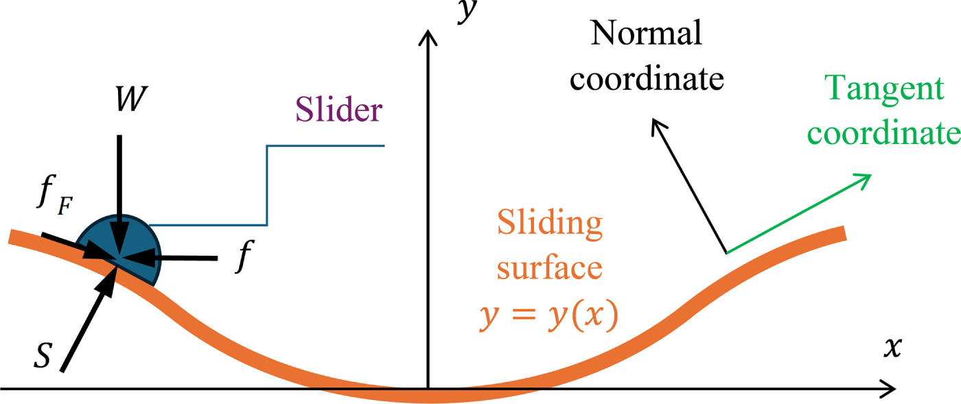
Figure 1: Free body diagram of the slider on the sliding surface, indicating the forces acting on the slider.

By formulating the equilibrium equations for the mentioned forces, the force-displacement relationship can be determined in a general form. Subsequently, by establishing equilibrium equations in the local coordinates, which are tangent and normal to the sliding motion, the force-displacement relationship at any given time moment can be expressed as follows [34]:

f=Wdydx+μWsgn(x˙)(1)

which signifies the restoring force Wdydx and the frictional force μWsgn(x˙) of the isolator system. In addition, μ denotes the friction coefficient between the slider and surface; sgn(x˙) is the sign function, assuming a value of +1 for positive sliding motion and −1 for negative sliding motion along the x-axis. Also, the friction coefficient of sliding isolators may depend on sliding velocity rather than remaining constant. Despite this variation, Eq. (1) for the VFPI remains applicable. However, the constant friction coefficient μ is substituted with μ(x), and an appropriate friction model that effectively characterizes the relationship between μ and x must be employed [51]. Subsequently, the stiffness of the VFPI based on the isolator displacement is obtained using the following equation:

k=k(x)=Wd2ydx2(2)

In addition, the isolator frequency may be simply given by:

ωb=ωb(x)=km=Wd2ydx2m=gd2ydx2(3)

where g denotes gravitational acceleration.

Eqs. (2) and (3) show that the stiffness and frequency of this isolator depend only on its geometry, and not on the isolated structure’s mass. This behavior stems from the gravity-based restoring mechanism of friction pendulum isolators rather than elastic deformation. As shown in the above equations, the stiffness depends on the curvature of the sliding surface and the vertical load, while the isolator frequency results from the ratio W/m, which simplifies to the gravitational acceleration g. Consequently, both stiffness and frequency are independent of the superstructure mass and are governed solely by the geometry of the sliding surface, allowing consistent isolator performance for different tank capacities and liquid levels. In simpler terms, this isolator exhibits a variable period or frequency that changes continuously with displacement. This inherent feature highlights the isolator’s adaptability and responsiveness across different levels of displacement, underscoring its versatility in seismic applications. Therefore, selecting the cross-sectional geometric function y(x) of the sliding surface, appropriately, allows the achievement of the desired hysteretic property and favorable dynamic characteristics.

3  Sliding Surface Functions

In this investigation, two different VFPI systems are analyzed in detail. The ensuing subsections provide a concise elucidation of the geometric characteristics of each.

3.1 Sixth-Order Polynomial Function

Lu et al. [34] proposed a 6th-order polynomial function to address resonant issues associated with FPS isolators. The new FPS isolator, called the Polynomial Friction Pendulum Isolator (PFPI), has an isolation frequency that varies with its displacement. Their proposed geometric function of the PFPI is given by:

y=(16)b1x6+(14)b2x4+(12)b3x2(4)

where b1, b2, and b3 are the polynomial coefficients. Next, using Eq. (1) and the first derivative of the above function, the force-displacement relationship can be written as follows:

f=Wdydx+μW=W(b1x5+b2x3+b3x+μ)(5)

The determination of the polynomial coefficients to meet specific design objectives is discussed in the subsequent sections.

3.2 Fourth-Order Polynomial Function

To achieve a PFPI with different mechanical properties, the geometric function of the PFPI can be expressed by the following 4th-order polynomial:

y=(14)c1x4+(12)c2x2(6)

Also, the force-displacement relationship of this isolator can be written as follows:

f=Wdydx+μW=W(c1x3+c2x+μ)(7)

4  Analysis of an Elevated Tank with an Isolation System

4.1 Mathematical Model

The schematic diagram of an elevated liquid storage tank with an isolation system can be represented by Fig. 2. As depicted, the elevated tank is isolated using two methods: firstly, by placing the bearings between the base of the tower structure and the foundation (referred to as isolated Model A), and secondly, by placing the bearings between the bottom of the liquid storage tank and the top of the tower structure (referred to as isolated Model B).

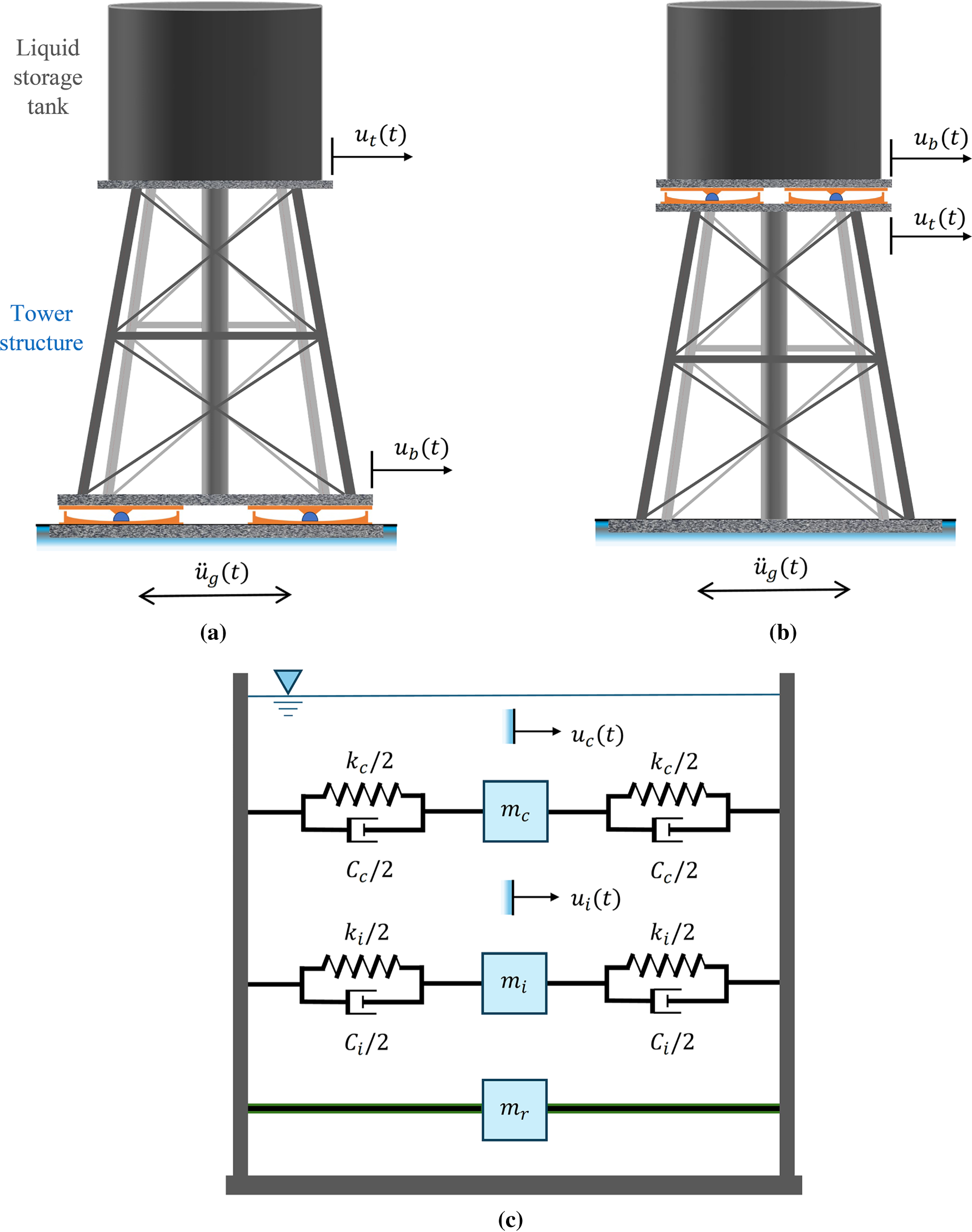
Figure 2: Structural model of elevated liquid storage tanks: (a) Model A, (b) Model B, and (c) the mechanical lumped-mass model of the tank.

This study employs a well-established, popular mechanical lumped-mass model [4] to evaluate the seismic response of the liquid storage tank. The total liquid mass, m, is divided into lumped masses known as sloshing, impulsive, and rigid masses, denoted as mc, mi, and mr, respectively [52]. The masses are computed following the equations provided below:

mc=Ycm(8)

mi=Yim(9)

mr=Yrm(10)

m=πR2Hρw(11)

in which Yc, Yi, and Yr indicate the dimensionless parameters [4], R denotes the tank’s radius, H is the liquid’s height, and ρw represents the liquid density. The lumped masses are connected to the tank wall via equivalent springs with stiffness constants kc and ki for sloshing and impulsive masses, respectively. Damping constants cc and ci are associated with these masses. For further information about the mechanical parameters indicated in Fig. 2, refer to Refs. [4,52].

Under the seismic excitation, the tank demonstrates three degrees of freedom, denoted as uc, ui and ut, representing the relative displacements of sloshing mass, impulsive mass, and tower drift, respectively. Notably, the presence of the isolation system introduces an extra degree of freedom to the tank’s dynamics, denoted as ub, which accounts for the deformation of the isolation system.

The equations of motion of an isolated elevated liquid storage tank subjected to ground motions are expressed in the matrix form as:

Mu¨(t)+Cu˙(t)+Ku(t)=f(t)−Mru¨g(t)(12)

where M, C and K are the mass, damping, and stiffness matrices, respectively. Also, r is the influence vector, and u¨g(t) is the ground acceleration component. Also, f(t) represents the vector of horizontal shear forces acting on the slider, including the restoring and friction forces, as extensively discussed in Section 4.2.

4.1.1 Model A

The relative displacement vector for Model A is given by u(t)=⌊uc(t)ui(t)ut(t)ub(t)⌋T, where the superscript T denotes the transpose. In this context, uc(t)=xc(t)−xt(t) introduces the displacement of the convective mass relative to the base of the tank, and ui(t)=xi(t)−xt(t) corresponds to the impulsive mass displacement with respect to the same reference point. In addition, ut(t)=xt(t)−xb(t) is the tower displacement relative to the isolator displacement, and ub(t)=xb(t)−ug(t) represents the relative displacement of the isolator system to the ground displacement. Furthermore, u˙(t) and u¨(t) denote the relative velocity and acceleration vectors, respectively.

The mass, stiffness, and damping matrices of Model A are given as follows:

M=[mc0mcmc0mimimimcmim+mbm+mbmcmim+mbm+mb+mt](13)

C=[cc0000ci0000ct0000cb](14)

K=[kc0000ki0000kt0000kb](15)

in which m denotes the total liquid mass, while the base mass is assumed to be 5% of the total liquid mass (i.e., mb=0.05m). Furthermore, the mass of the steel tower structure is assumed to be 10% of the total liquid mass (i.e., mt=0.1m) [12]. Moreover, the tower’s dynamic properties are computed in accordance with an equivalent single-degree-of-freedom (SDOF) system as indicated by:

kt=1.05m(2πTt)2(16)

ct=2ξt(1.05m)ωt(17)

in which Tt and ξt indicate the time period and damping ratio of the tower. Also, ωt refers to the tower’s frequency. Similarly,

kb=1.15m(2πTb)2(18)

cb=2ξb(1.15m)ωb(19)

where Tb, ξb and ωb are the time period, the damping ratio, and the frequency of the isolation system. Moreover, the influence vector of Model A is written as follows:

r=⌊0001⌋T(20)

4.1.2 Model B

Similarly, the relative displacement vector for Model B is denoted by u(t)=⌊uc(t)ui(t)ub(t)ut(t)⌋T, where uc(t)=xc(t)−xb(t), ui(t)=xi(t)−xb(t), ub(t)=xb(t)−xt(t), and ut(t)=xt(t)−ug(t). The mass, stiffness, and damping matrices of Model B are written as:

M=[mc0mcmc0mimimimcmimmmcmimm+mt](21)

C=[cc0000ci0000cb0000ct](22)

K=[kc0000ki0000kb0000kt](23)

Similar to Model A, it is assumed that mb=0.05m and mt=0.1m. Furthermore,

kt=1.1m(2πTt)2(24)

ct=2ξt(1.1m)ωt(25)

kb=m(2πTb)2(26)

cb=2ξbmωb(27)

r=⌊0010⌋T(28)

It should be noted that the adopted lumped-mass formulation, based on Haroun’s well-established model [4], is a popular mechanical model that accounts for wall flexibility. This model has been extensively validated through boundary element analyses, experimental data [4], and comparisons with simplified procedures recommended by well-known standards such as the American Petroleum Institute (API). These industry guidelines provide practical procedures for estimating seismic forces without modeling every detail. This well-established representation was adopted in this study to enable parametric investigation and optimization of the PFPI surface function across a wide range of seismic intensities and geometric configurations.

4.1.3 Friction Mechanism

Frictional resistance at sliding interfaces is the primary mechanism for energy dissipation during motion. The response of friction bearings can be described in terms of two distinct phases: the non-sliding phase and the sliding phase. In the non-sliding phase, the structure remains stationary relative to the sliding surface, as the vibration-induced shear force does not exceed the maximum available friction force. Once this threshold is reached, the bearing enters the slip phase, during which relative motion occurs, and energy is dissipated through friction. In summary, the non-sliding conditions require that:

|f(t)|<μ(t)W(29)

and

u˙b(t)=0(30)

Sliding conditions arise solely when:

f(t)=μ(t)Wsgn[u˙b(t)](31)

u˙b(t)≠0(32)

in which the friction coefficient μ(t) varies depending on the material. This coefficient is contingent upon the sliding velocity and bearing pressure, as given by [25]:

μ(t)=μmax−(μmax−μmin)exp⁡[−a|u˙b(t)|](33)

where μmax and μmin represent the maximum and minimum values of the friction coefficient, respectively. Also, u˙b(t) denotes the sliding velocity of the bearing, and the coefficient a is determined based on the bearing pressure and is taken as a=20 s/m [51].

4.2 Numerical Procedure for Sliding Systems

The governing equations of motion differ between the two phases, leading to highly nonlinear behavior. The overall motion can be viewed as a sequence of non-sliding and sliding phases. Notably, the equation of motion is linear in the non-sliding phase and nonlinear in the sliding phase. Given the continuous transition between phases as the isolator force magnitude varies, the overall dynamic behavior is generally nonlinear. Therefore, the equations of motion (12) can be reformulated in the following form:

Mu¨(t)+Cu˙(t)+Ku(t)=bf(t)+Ew(t)(34)

to be cast in a state-space representation as a numerical nonlinear solution method. The first term on the right side of Eq. (12) has been replaced by bf(t), where b represents the 4 × 1 location vector of the friction force. Also, Ew(t)=−Mru¨g(t), where E indicates the 4 × 4 location matrix of the external loads generated by lumped masses, and w(t) is the 4 × 1 loading vector. Moreover, the friction force should satisfy Eqs. (29)–(32). Now, Eq. (34) can be rewritten as a first-order differential equation [53]:

z˙(t)=A∗z(t)+E∗w(t)+b∗f(t)(35)

in which the 8 × 1 state vector is given by:

z(t)={u(t)u˙(t)}(36)

Also, the 8 × 8 system matrix is as follows:

A∗=[0I−M−1K−M−1C](37)

In addition, the 8 × 4 placement matrix for the ground excitations is written as:

E∗=[0M−1E](38)

The 8 × 1 vector for the VFPI forces is represented by the following expression:

b∗={0M−1b}(39)

By employing first-order interpolations of the loading terms between two consecutive sampling instants, the state Eq. (27) can be further resolved as a different equation:

z(tk)=Az(tk−1)+b0f(tk−1)+b1f(tk)+E0w(tk−1)+E1w(tk)(40)

where, tk and tk−1 represent the current and previous time steps, respectively. In other words, tk=tk−1+Δt. Also, A=exp⁡(ΔtA∗) indicates the 8 × 8 exponential matrix of the discrete time system with time intervals Δt. Next, the coefficient vectors in Eq. (40) are calculated from the following relationships:

b0=[(A∗)−1A+1Δt(A∗)−2(I−A)]b∗(41)

b1=−[(A∗)−1+1Δt(A∗)−2(I−A)]b∗(42)

In addition, the coefficient matrices are:

E0=[(A∗)−1A+1Δt(A∗)−2(I−A)]E∗(43)

E1=−[(A∗)−1+1Δt(A∗)−2(I−A)]E∗(44)

The discrete-time state-space Eq. (40) highlights that the friction force, f(tk), at the current time instant tk is contingent upon motion conditions that are not predetermined. As a result, obtaining the solution through straightforward recursive calculations is impractical. Rather than resorting to the common iterative corrective pseudo-force approach used in nonlinear dynamic analyses, a methodology rooted in the concept of shear balance at sliding interfaces is proposed in the following section.

4.3 Shear Balance Procedure

The friction mechanism elucidates that the motion conditions are represented by the base shear force and the sliding velocity of the base floor. During the sliding phase, the friction force is governed by Eq. (29), while the sliding velocity remains unknown. Conversely, in the non-sliding phase, the sliding velocity at the base floor is zero, as defined by Eq. (30), yet the base shear remains indeterminate. In general, either the base shear or sliding velocity is ascertainable, contingent upon the prevailing motion condition. This additional constraint enables the determination of the base shear, f(tk), uniquely at time instant tk.

Initially, establishing a non-sliding condition for the system at the time instant tk yields:

u˙b(tk)=Dz(tk)=0(45)

in which D=⌊0bT⌋ denotes the 1 × 8 location vector of the base velocity. Substituting Eq. (40) for z(tk) into Eq. (45), the base shear force required to prevent the system from sliding can be determined in closed form as:

f~(tk)=−(Db1)−1D{Az(tk−1)+E0w(tk−1)+E1w(tk)+b0f(tk−1)}(46)

Based on the friction law, f~(tk) must not exceed the maximum friction force.

The first step is to compare the calculated value and the maximum friction force. If |f~(tk)|<μW, it means that the initial assumption of the non-sliding phase in the analysis is validated; furthermore, the friction force is updated as f(tk)=f~(tk). If |f~(tk)|≥μW, the system would enter a sliding phase instead, necessitating an adjustment of the friction force to align with f(tk)=μWsgn(f~(tk)).

As the next step, the system response z(tk) can be calculated using the obtained force f(tk). According to Mokha’s model [25], the solution requires an iterative approach to determine the correct friction coefficient during sliding. Therefore, the friction coefficient μ¯ should be obtained according to the sliding velocity u˙b(tk)=Dz(tk). If |(μ¯−μ)/μ|≤errallow, where errallow is the allowable error, the solution is validated. If |(μ¯−μ)/μ|>errallow, the friction force should be revised as f(tk)=μ¯Wsgn(u˙b(tk)), set μ¯=μ, and then return to the first step of the loop.

5  Optimization Algorithms

An engineering optimization problem typically involves two main phases: first, the mathematical formulation of the problem, and second, its computational execution. Mathematical and computational techniques are employed to identify the optimal solution from a range of feasible options, focusing on objective functions, decision variables, and constraints. An optimization problem requires a clear understanding of its specifics, appropriate metric selection, and consideration of computational complexity, while avoiding pitfalls such as unclear objectives and neglecting real-world constraints. Furthermore, the computational implementation requires a suitable optimizer and a computationally efficient numerical model of the structure. This involves selecting or developing algorithms that can effectively navigate the design space to find the optimal solutions. Popular optimization techniques include gradient-based methods, genetic algorithms, and swarm intelligence approaches, among others.

In this study, various swarm-based optimization algorithms are implemented to determine the optimal geometric function of a VFPI. These techniques emulate the collective intelligence seen in swarms and flocks. In fact, the primary characteristic of swarm-based methods is the coordinated behavior and instinct-driven actions of herds. The two well-known optimizers in this category include cuckoo search (CS) and bird swarm algorithm (BSA). The selection of these algorithms is rooted in their distinct strengths and synergistic characteristics, which effectively address the complexities associated with optimizing the geometric parameters of VFPIs. CS provides robust global search capabilities, excelling in avoiding local optima. Also, BSA uses role diversity to balance exploration and exploitation. Together, these methods offer a reliable framework for navigating the nonlinear VFPI design space, ensuring accuracy and robustness under diverse seismic conditions.

5.1 Cuckoo Search (CS)

The intriguing behavior of particular bird species, particularly their aggressive reproduction strategy, has inspired the development of the CS algorithm [54]. This algorithm draws its inspiration from the unique breeding behavior of cuckoos, especially their brood parasitism. Instead of building their own nests, some species of cuckoos lay their eggs in the nests of other bird species. In this algorithm, potential solutions are represented as eggs and nests, mimicking natural behavior to optimize complex problems.

In CS, when generating a new solution xik+1 form its previous solution xik, for a cuckoo i, a Lévy flight is performed, enhancing exploration of the search space. The high-quality solutions (eggs) are then carried over to the next generation. The algorithm operates based on three idealized rules:

(i)   Single egg laying. Each cuckoo lays one egg at a time and places it in a randomly chosen nest.

(ii)   Survival of the fittest. The nests containing the best-quality eggs are carried over to the next generation.

(iii)   Fixed host nests and discovery probability. The number of available host nests is fixed. If a host bird discovers an alien egg with a probability Pa∈[0,1], it can either throw the egg away or abandon the nest and build a new one.

In a maximization problem, the value of the objective function is proportional to the quality or fitness of each solution (design). As mentioned earlier, a simple representation is used where each egg in a nest corresponds to a single design, and each cuckoo lays only one egg, representing a new design. The objective is to replace less optimal solutions in the current generation with new, potentially better ones (cuckoos). This fundamental principle can be extended to more complex scenarios where each nest contains multiple eggs, representing a set of possible solutions. In CS, a balanced combination of a global and a local explorative random walk is utilized, which is controlled by Pa.

The local random walk is achieved based on the following relationship:

xik+1=xik+α.S⊗H(Pa−ϵ)⊗(xjk−xlk)(47)

in which k refers to the do-loop variable, S represents the step size, and α>0 denotes the step size scaling factor, which should be appropriately set to match the problem at hand. In most scenarios, α can be set to 1. In addition, ⊗ indicates the entry-wise product of two vectors, H(⋅) is the Heaviside function, and ϵ implies a random number following a uniform distribution. Also, xjk and xlk show two various solutions randomly chosen by arbitrary permutations.

For the global random walk, Lévy flights are performed for generating new solutions as given below:

xik+1=xik+α.Le´vy(λ,S)(48)

where,

Le´vy(λ,S)=λ.Γ(λ)πS1+λsin⁡(πλ2)(49)

in which λ represents the occurrence mean of an event during a unit interval, and Γ(⋅) is the standard Gamma function.

Eq. (48) essentially represents a stochastic equation for a random walk. Generally, a random walk is a Markov chain in which the next state or position depends only on the current position (indicated by the first term in Eq. (48)) and the transition probability (represented by the second term). However, the random walk conducted via Lévy flight proves more efficient for exploring the search space, as it allows longer step lengths over iterations. Lévy flights are advantageous because they allow longer step lengths, helping the algorithm avoid local optima and thereby increasing the likelihood of finding a global optimum.

5.2 Bird Swarm Algorithm (BSA)

BSA is inspired by the social behavior of birds as they forage for food, avoid predators, and navigate through their environment [55]. BSA models these behaviors to solve optimization problems, assigning different roles to swarm members to mimic the natural flocking strategies of birds. BSA divides the flock into various roles, as follows:

(a)   Producers. These birds explore the search space to find food (optimal solutions) and lead the swarm towards promising areas.

(b)   Scroungers. These birds follow the producers and exploit the food sources they discover. They intensify the search around known reasonable solutions.

(c)   Rangers. These birds explore new regions of the search space to avoid local optima, ensuring the algorithm maintains population diversity.

BSA also incorporates behavioral switches, enabling birds to switch roles in response to the swarm’s needs, thereby ensuring adaptability and robustness in the search process. In BSA, the behavior of producers and scroungers is inspired by the natural foraging patterns of birds. Producers are responsible for actively searching for food, while scroungers benefit from producers’ efforts by consuming the food producers find. This dynamic allows each bird to leverage social interactions, ensuring a low-risk search strategy and enhancing the overall chances of survival.

BSA simplifies these social behaviors with several key rules:

(i)   Each bird alternates between vigilance (awareness of surroundings) and food-searching behaviors, with these behaviors modeled as random decisions.

(ii)   While searching for food, each bird records both its own best experience (best position) and the group’s best experience, sharing this information with the entire flock.

(iii)   During vigilance, birds tend to move towards the center of the group, with those having more resources positioning themselves closer to the center.

(iv)   Periodically, birds migrate to new locations. In these scenarios, birds with the most reserves become producers, while those with the fewest reserves become scroungers. Birds with intermediate reserves are randomly assigned as either producers or scroungers.

(v)   Producers actively search for food, and scroungers follow a producer randomly to take advantage of the food discovered.

This strategy ensures that the flock can efficiently explore the search space while minimizing risk, reflecting the balance of exploration and exploitation inherent in BSA.

The BSA algorithm starts with a population of birds, each representing a potential solution. The birds are divided into different roles, and their movements are governed by the strategies associated with their roles. Producers explore the solution space, scroungers exploit the areas found by producers, and rangers ensure diversity by exploring new regions. The algorithm iteratively updates the birds’ positions, with the swarm converging to the optimal solution over time. The adaptive role-switching mechanism enables BSA to dynamically adjust its search strategy in response to the problem landscape. Further details may be found in Ref. [55].

6  Optimization Formulation

As mentioned before, the force created in a PFPI system is expressed by Eq. (1). Also, the acceleration based on Newton’s second law is defined as follows:

f=mas(50)

where as represents the accelerations transmitted to the superstructure. It is important to highlight that for a VFPI system, the optimization function focuses on reducing the accelerations transmitted to the superstructure. Therefore, to achieve the appropriate optimization function, it is recommended to combine Eqs. (1) and (50). Therefore, the transferred acceleration function to the superstructure, to be minimized, is expressed in the following equation:

as=(dydx+μ.sgn(x˙))g(51)

Building on this, a novel optimization function has been developed in this study that incorporates the first derivative of the surface curve for PFPI systems introduced previously. By assuming D as the maximum displacement capacity of the isolator, the objective function for optimization—specifically, minimizing the maximum acceleration transferred to the superstructure—can be formulated for three types of VFPI systems. For the 6th-order polynomial function, the maximum transferred acceleration is obtained by assuming x=D, sgn(x)=1, and sgn(x˙)=1 as follows:

as6th−order=(b1D5+b2D3+b3D+μ)g(52)

Similarly, for the 4th-order polynomial functions, one may write:

as4th−order=(c1D3+c2D+μ)g(53)

These formulations provide a tailored approach to optimizing PFPI performance. It was shown that the mechanical properties of a VFPI system can be customized by adjusting the coefficients in its sliding surface function [56]. It is worth noting that these functions are symmetric about the y-axis and pass through the origin of the coordinate system.

To make the design process more practical, the mathematical coefficients of Eqs. (52) and (53) should first be translated into parameters that hold more significance from an engineering perspective. This approach will then be applied to design prototype VFPI isolators for testing in the experiment [56]. For instance, the following engineering parameters for a 6th-order VFPI isolator are considered: (a) k0 which denotes the normalized initial stiffness at x=0, (b) D1 and D2 which represents the isolator displacement at points 1 and 2 (see Fig. 3), and (c) k1 and k2 which refers to the secant stiffness at points 1 and 2.

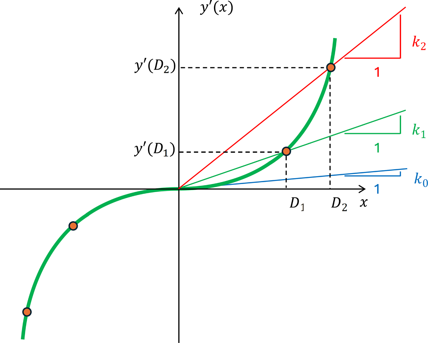
Figure 3: The first derivative of y(x) in conjunction with k0, k1, and k2.

The normalized stiffness can be obtained from Eq. (2) as follows [56]:

k¯(x)=1Wk(x)=1Wddx(Wd2ydx2)=y′′(x)(54)

Therefore,

k0=k¯(x=0)=y′′(x=0)(55)

Moreover,

k1=y′(D1)D1(56)

k2=y′(D2)D2(57)

Next, by substituting y(x) from Eq. (4) into Eqs. (55)–(57), it is possible to solve the three simultaneous equations and determine the values of the coefficients as follows:

b1=(D2D1)2(k0−k1)+k2−k0D12D22[(D2D1)2−1](58)

b2=(D2D1)4(k1−k0)+k0−k2D22[(D2D1)2−1](59)

b3=k0(60)

The same calculations can be followed to find the corresponding coefficients for the 4th-order function.

To illustrate how the mentioned design parameters are determined for the prototype VFPIs used in the experiment [56], let’s first assume that the secant stiffness k¯(x) of the isolators increases monotonically as the isolator displacement increases. This assumption suggests that k0<k1<k2 (with corresponding periods T0>T1>T2). Additionally, let D1, D2 represent the allowable isolator displacements corresponding to two design earthquakes of low and high intensity, respectively. Similarly, k1 and k2 represent the desired isolator stiffness values at the specified displacements, respectively. In practice, the two levels of earthquakes can correspond to those established in various design codes, such as the design basis earthquake (DBE) and maximum considered earthquake (MCE) outlined in the International Building Code. With the allowable values of D1 and D2 for earthquakes of varying intensities, two performance objectives can be integrated into the VFPI design. First, for lower-intensity earthquakes in which the isolator displacement remains below D1, the goal is to protect the isolated object by minimizing its acceleration response (or, acceleration control). To achieve this, a longer isolation period T1 (i.e., lower stiffness k1) is preferred. Second, for higher-intensity earthquakes in which the isolator displacement exceeds D1 and may approach D2, the focus shifts to displacement control to prevent excessive movement and potential pounding issues. In this scenario, a shorter isolation period T1 (i.e., higher stiffness k1) is necessary. Consequently, the VFPI’s restoring force function will feature a softening section (where stiffness decreases to reduce acceleration during moderate earthquakes) followed by a hardening section (where stiffness increases to limit displacement during severe earthquakes).

Therefore, it is necessary to establish an acceptable range for the permissible displacement D1 and the initial stiffness k0. These parameters can then be used in optimization algorithms to determine the coefficients related to the surface function of the isolator curve, ultimately reducing the acceleration transmitted to the structure. Based on this, the permissible displacement is defined as the maximum displacement of an isolated system according to clause 17.5.3.1 of the ASCE/SEI 7-22 standard, as follows:

DM=gSM1TM4π2BM(61)

in which TM is the effective period, SM1 indicates the spectral acceleration at a period of 1 s based on clause 11.4.4 or 11.4.8, and BM denotes the damping reduction factor determined in accordance with Table 17.5-1 of this standard. Given the soil type at the site and the assumption that TM=T0, knowing the range for the initial period of the isolator allows for determining the range of DM, or D1, which is necessary to achieve an optimal isolator design.

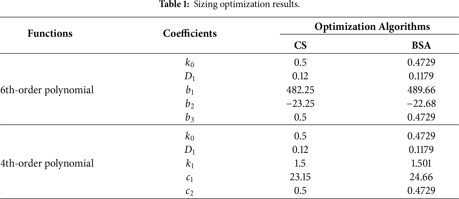
The optimization framework used in this study is briefly described here to provide a clearer, more explicit presentation. The optimization problem is formulated to identify the optimal geometric parameters of the PFPI surface, which serve as design variables and define the polynomial representation of the isolator geometry. The objective function is defined as the minimization of the peak seismic response transmitted to the superstructure, evaluated through nonlinear time history analysis, as reported in Table 1. The optimization is subject to a set of displacement- and stability-related constraints, all of which are satisfied in the optimal solutions obtained by both metaheuristic optimization algorithms. This framework links the isolator geometry to the effective dynamic properties of the system and enables the use of techniques to search for optimal solutions.

The optimal surface functions for isolators with 4th-order and 6th-order functions are determined using the proposed process, along with the primary frequency of the system. The primary frequency of this type of isolator is calculated using Eqs. (3), (4) and (6). By leveraging the relationships between the period and frequency of the system, the optimal configuration of this isolator can be achieved by determining the range for maximum displacement and the period, and by employing optimization algorithms.

Further analysis of the proposed relationships for achieving the optimal surface function of PFPIs reveals that these relationships are independent of the structure’s weight. Therefore, it is essential to note that changes in the volume and height of the liquid within the tank do not affect the optimal surface function obtained using the proposed relationships.

7  Dynamic Analyses and Record Selection

To evaluate the behavior of the proposed isolators, the model parameters are considered as follows: the liquid height H=5 m, and the wall thickness-to-tank radius ratio is 0.004. Also, the liquid’s height-to-tank radius ratio (H/R) is 0.6 and 1.85 for the broad and slender tanks, respectively. The sloshing and impulsive frequencies for the broad tank are 0.148 and 5.575 Hz, respectively. For the slender tank, the corresponding frequencies are 0.291 and 6.738 Hz, respectively. The period of the steel tower structure Tt is assumed to be 1 s. The damping ratio of the isolation system ξb is considered to be 10%.

Investigation and analysis of damage reveal that ground motions with long periods have a more destructive impact on structures like tall buildings, isolated structures, and storage tanks, due to the increased likelihood of resonance. As previously explained, base isolation increases the fundamental period of a structure, making the study of isolated structures under the influence of long-period earthquakes significant. Among the most damaging earthquakes are the 1985 Mexico City earthquake, 400 km from the epicenter, and the Tokachi earthquake in Japan in 2008 [57].

The nature of an earthquake and its seismic movements depend on site characteristics, the propagation path, and local domain effects. Typically, ground motions with a dominant period of 1 s or less are classified as short-period ground motions. In contrast, those with a dominant period between 1 and 10 s are considered long-period ground motions. Initially, the dominant period of an earthquake was used to indicate part of its spectral characteristics. However, this parameter is limited because it cannot fully describe the spectrum around the peak or the overall shape of the spectrum. Additionally, when a spectrum has multiple peaks, small changes in the ground motion can significantly alter the dominant period.

Another approach defines long-period ground motions based on the characteristics of the ground motion time history, identifying pulse-like features or simple harmonic vibrations as indicative of long-period motions. Recently, researchers have introduced additional parameters, including time-domain and frequency-domain parameters, to better identify long-period ground motions. These new methods classify ground motions using ground motion data rather than traditional seismological parameters. For example, Zhou et al. [58] developed an improved frequency range parameter to characterize long-period motions, which does not rely on seismic data but instead uses statistical analysis of 39,744 strong ground motions from the PEER database. This parameter, which is also called Zhou’s criterion, is obtained from the following relationship:

βl=∑Tiαβα(Ti)∑Tiα(62)

where βα is the value of the response spectrum of the normalized acceleration of the ground motion. Also, Ti indicates the i-th interval time in the range of 1 to 10 s with intervals of 0.01 s, and Tiα is the weight coefficient of the value of the βα(Ti) spectrum. Zhou et al. [58] calculated the value of βl for all 39,744 earthquake records, and based on their analysis, α=0.6 was identified. If βl≤0.4, the earthquake is a normal ground motion. For 0.4<βl<0.6, the earthquake is considered a medium–long-period one; and if βl≥0.6, the earthquake is assumed to be long-period.

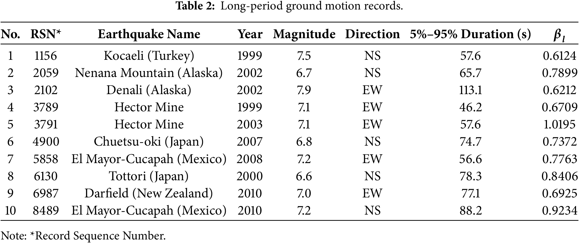
According to the above explanations, first, the selected records were checked against Zhou’s criteria, and then they were classified as long-period earthquakes according to Table 2.

8  Numerical Results

8.1 Optimization Results

As previously discussed, the optimal properties of the 6th-order and 4th-order PFPI have been determined using two optimization algorithms, considering the objective functions and constraints outlined earlier. The optimization results are presented in Table 1 for the two isolator types.

As shown in Table 1, the optimal objective function values obtained by the two optimization algorithms, CS and BSA, are nearly identical, despite using different combinations of design variables, and all constraints are met. It is essential to note the variations in constraint values that arise from their highly nonlinear nature. Even small fluctuations in the design parameters (e.g., coefficients of the isolator surface function) can lead to significant differences in constraint function values, increasing the problem’s complexity and making it more challenging for the algorithms to achieve the global optimum.

Fig. 4 illustrates the convergence histories for the optimization algorithms across the two isolator types. Regarding computational efficiency, CS achieved faster convergence for both isolators, outperforming the other algorithm. This behavior highlights the effectiveness of CS in maintaining stability and efficiency, while BSA, despite its exploration capabilities, was more susceptible to converging at suboptimal solutions. In other words, BSA exhibited a higher objective function value, further reinforcing the challenge of escaping local minima in complex optimization landscapes.

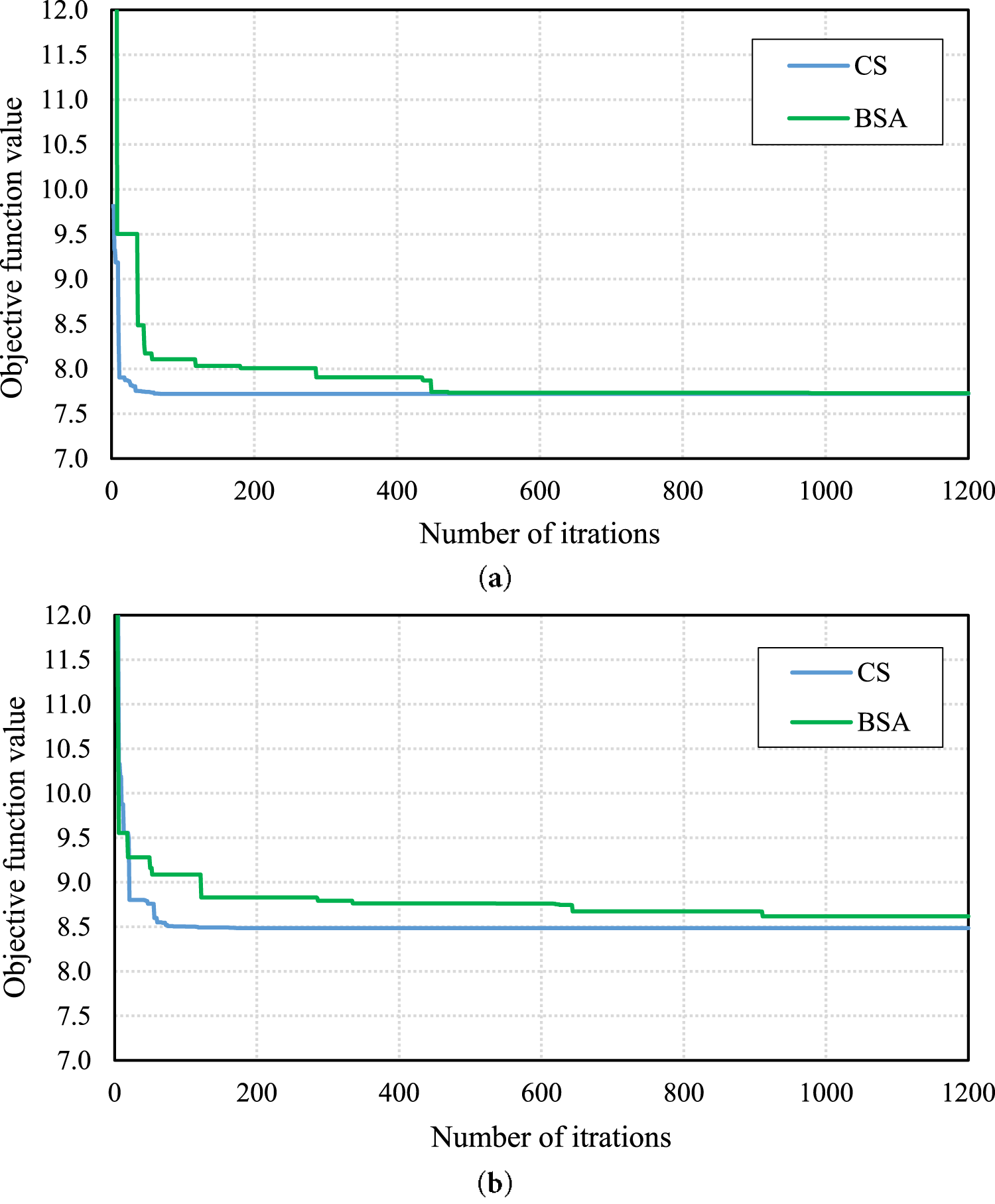
Figure 4: The optimization algorithms’ convergence histories for (a) the 6th-order, and (b) the 4th-order VFPI isolators.

8.2 Time History Results

This section evaluates the seismic performance of base-isolated (Models A and B) and non-isolated elevated liquid storage tanks using the optimized isolators identified in Section 8.1 (summarized in Table 3). As a representative strong near-fault ground motion, the 1994 Northridge–01 earthquake record is employed to evaluate the nonlinear response of the isolated systems, and the corresponding responses of broad tanks are presented in Figs. 5 and 6. The top inserts of these figures depict the time history variations of convective mass acceleration, illustrating the effectiveness of the isolation systems in mitigating dynamic demands. Observations indicate that seismic isolation leads to substantial attenuation of both structural and hydrodynamic responses compared to the non-isolated case.

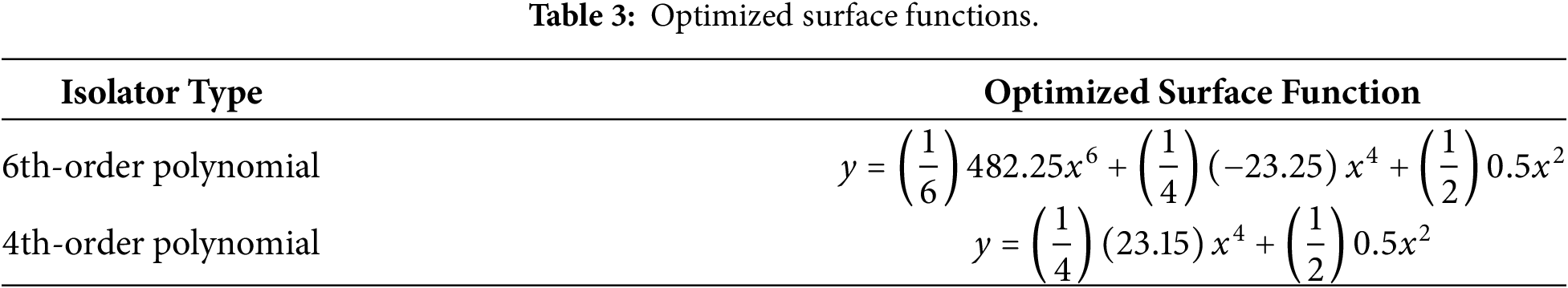
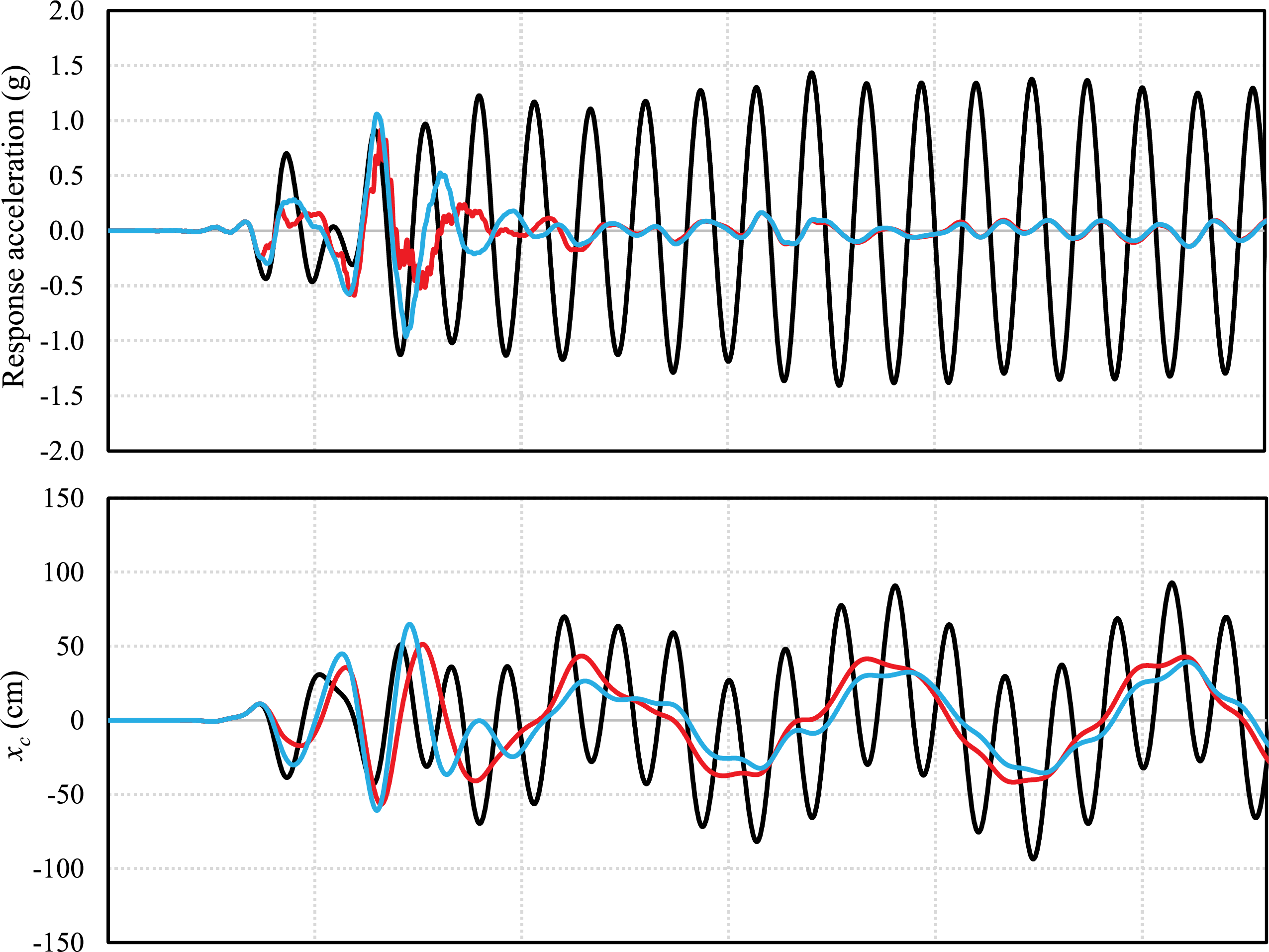
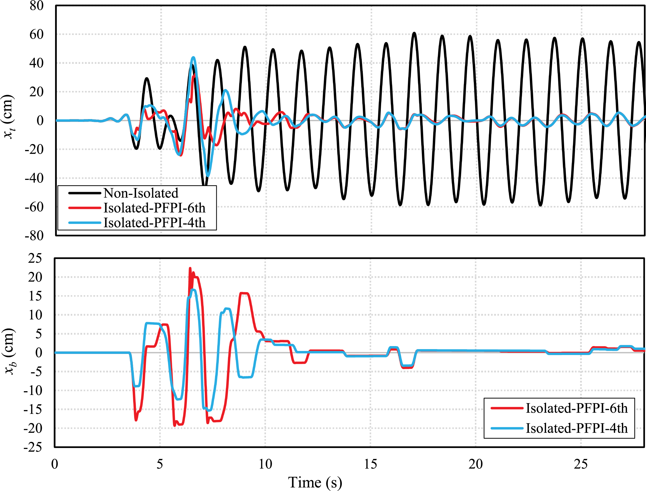
Figure 5: The top insert shows the time history of convective mass acceleration for the broad elevated liquid storage tank (Model A) subject to the 1994 Northridge-01 seismic record (RSN = 982) NS component. Also, time histories of convective mass displacement xc(t), the tower displacement xt(t), and the isolator displacement xb(t) are shown.

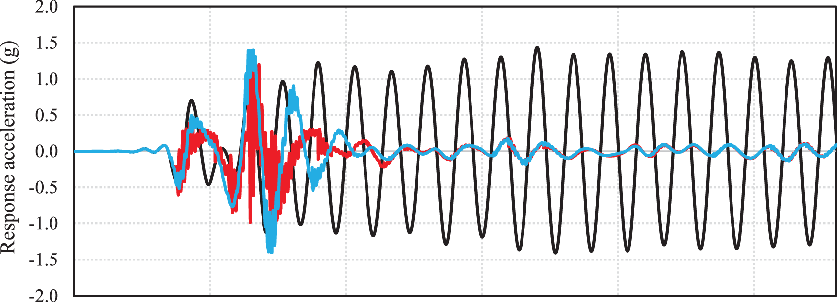
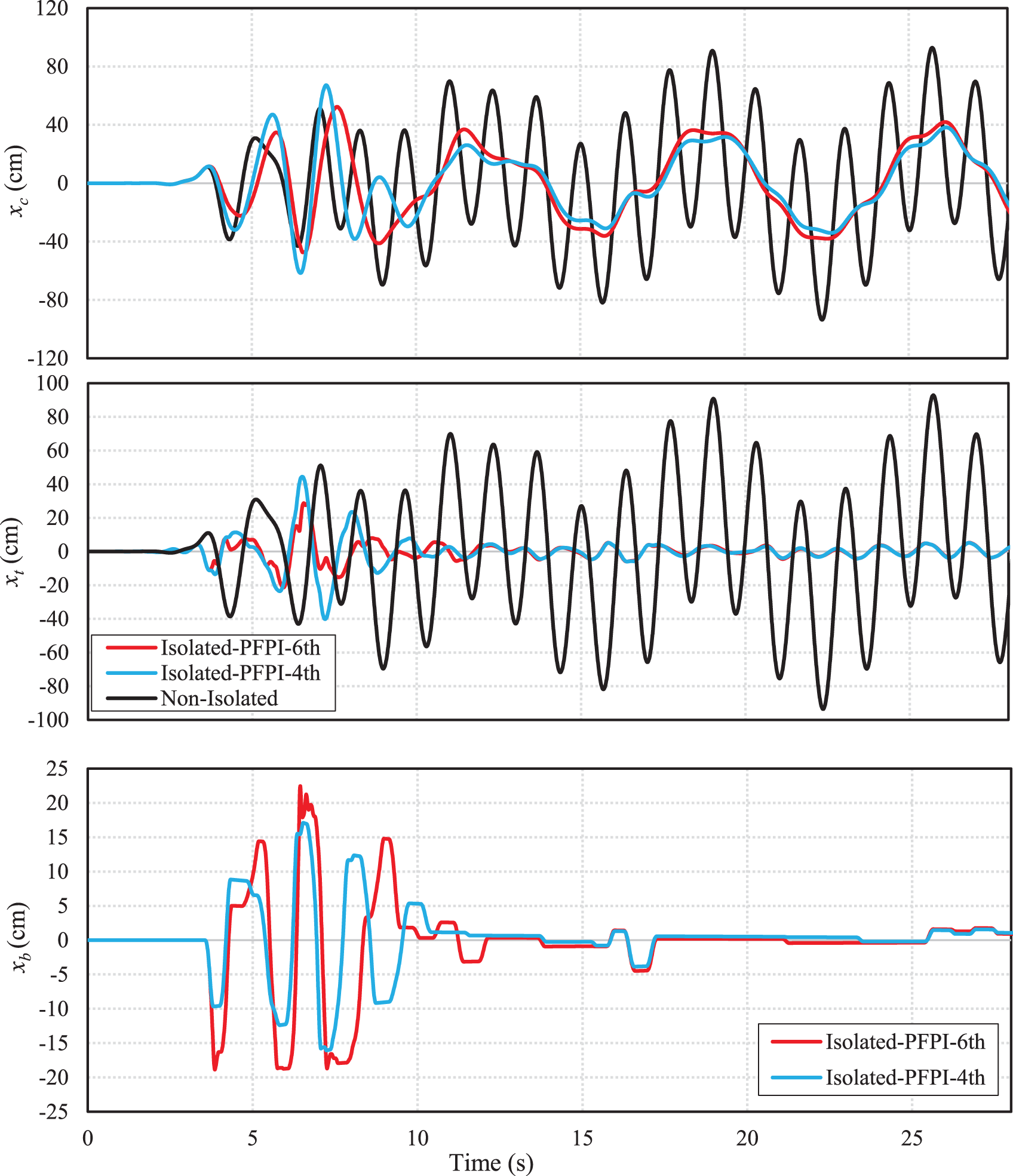
Figure 6: The top insert shows the time history of convective mass acceleration for the broad elevated liquid storage tank (Model B) subject to the 1994 Northridge-01 seismic record (RSN = 982) NS component. Also, time histories of convective mass displacement xc(t), the tower displacement xt(t), and the isolator displacement xb(t) are shown.

In addition, Figs. 5 and 6 indicate the time variations of three displacements, xc(t), xt(t), and xb(t) for Models A and B, respectively. Also, the maximum responses are summarized in Table 4.

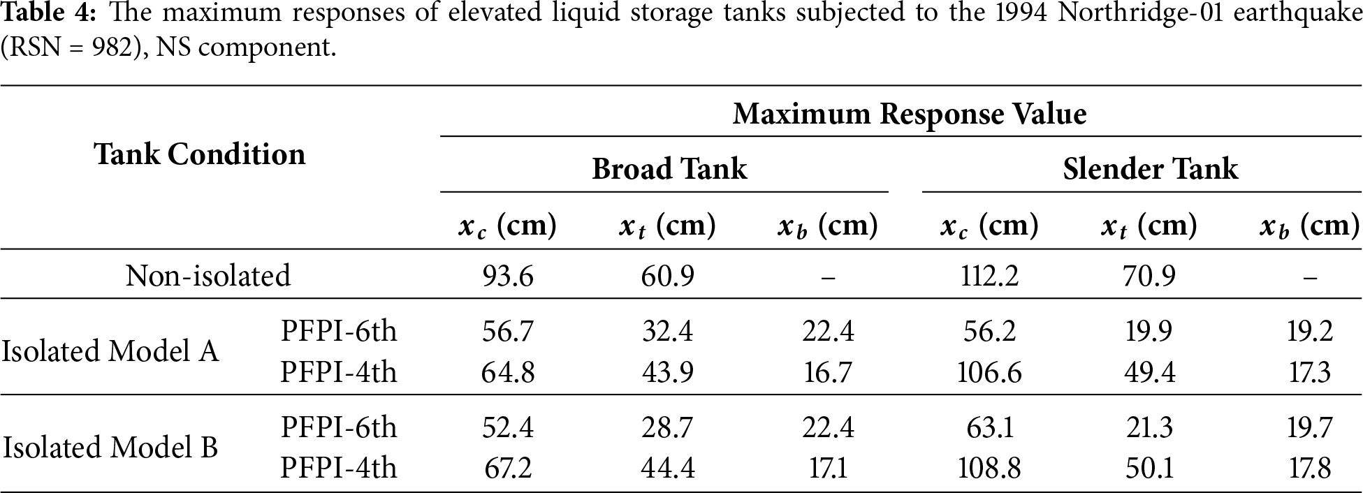
As shown in Table 4, the implementation of the PFPI-6th isolation system in Model A reduces the maximum convective mass displacement for broad tanks by approximately 39% compared to non-isolated benchmarks. This mitigation is even more substantial for slender tanks, where convective displacement decreases by nearly 50%. Tower displacement demonstrates an even sharper decline, with reductions of roughly 47% for broad tanks and over 72% for slender configurations under PFPI-6th isolation. While both PFPI-4th and PFPI-6th variants provide protection, the 6th-order model consistently offers superior control over structural and liquid oscillations. In Model B specifically, adopting the PFPI-6th system instead of the PFPI-4th yields an additional 22% reduction in convective displacement for broad tanks. It is observed that while structural and convective responses are minimized, isolator displacement is maintained at levels that ensure the overall stability of the base. The comparative data suggest that slender tanks experience the most significant relative benefits from isolation in terms of tower integrity. Ultimately, these results demonstrate that advanced friction pendulum isolators are highly effective at suppressing both hydrodynamic sloshing and structural vibrations during intense seismic events.

8.3 Long-Period Earthquakes

As previously established, the implementation of base isolation in elevated liquid storage tanks significantly attenuates the seismic accelerations transmitted to the superstructure, effectively reducing the global seismic demand. This mitigation ensures that the tank remains predominantly within the linear elastic range under most design-level earthquake scenarios, thereby minimizing the probability of severe structural damage at high PGA levels. However, as seismic intensity escalates—particularly during the higher scaling stages of the Incremental Dynamic Analysis (IDA)—acceleration demands can increase substantially. These elevated responses are a function of both the isolation configuration and the specific frequency content and duration characteristics of the long-period seismic inputs, which can induce higher-mode effects or resonance in the isolated system.

To examine this behavior, the maximum convective acceleration responses, already mitigated by isolation, were extracted and compared for the optimized configurations introduced in Section 8.1 and the conventional configurations, listed in Table 5. These comparisons were conducted for both isolation layouts, Model A and Model B. Figs. 7 and 8 illustrate these comparisons for both slender and broad tank geometries, using 10 long-period ground motion records.

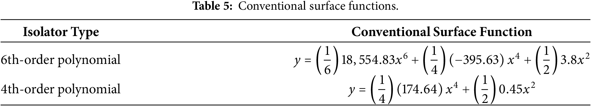
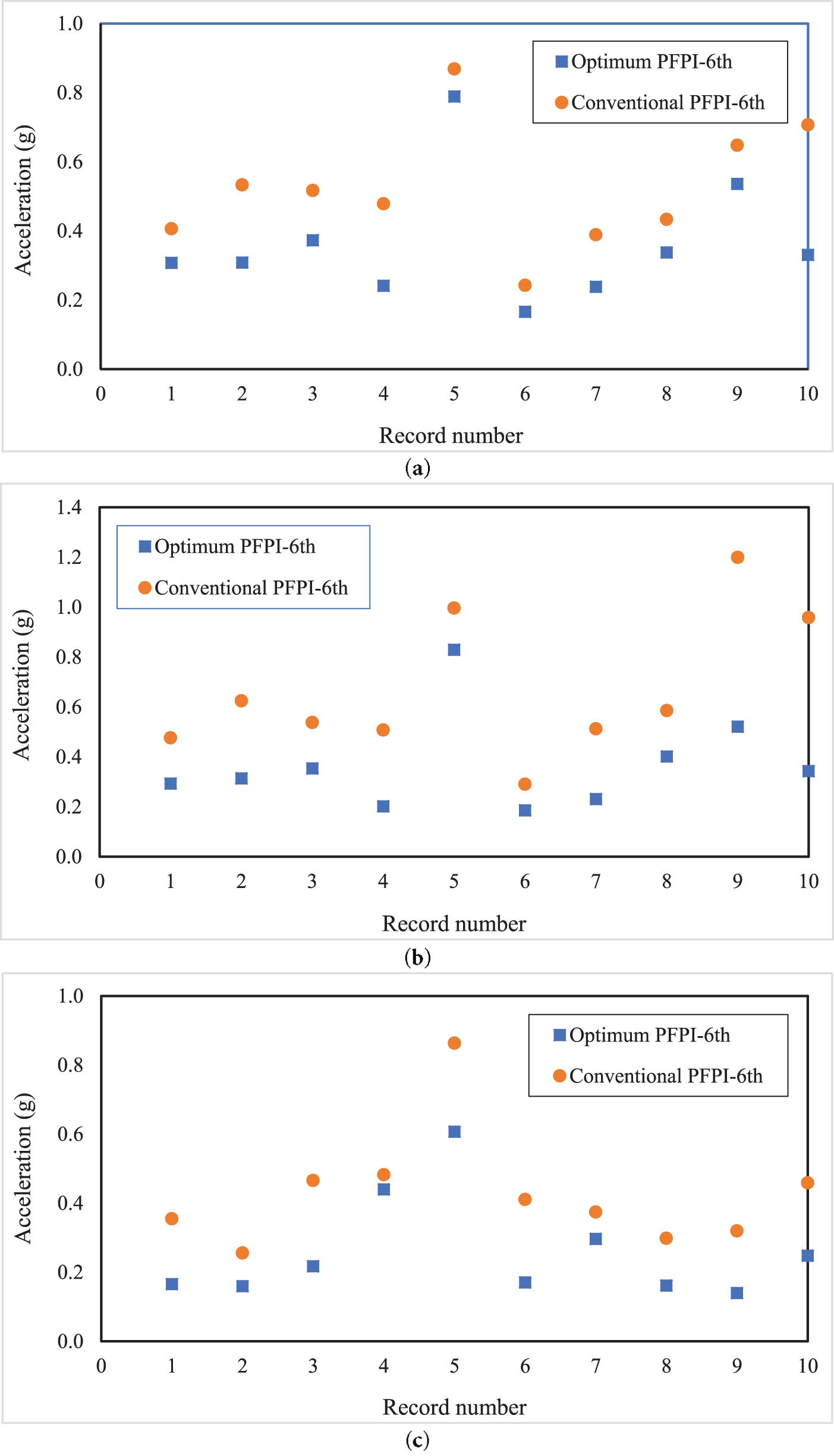
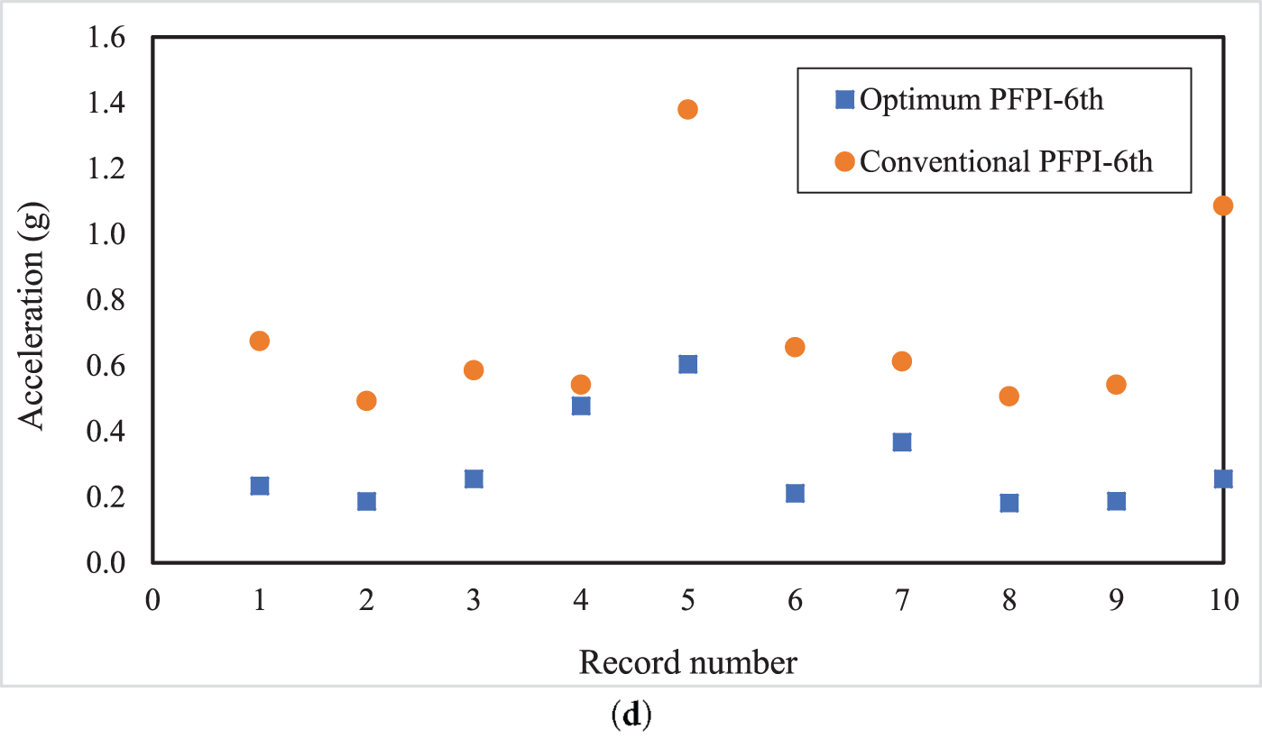
Figure 7: The maximum convective acceleration responses for the optimum and conventional 6th-order PFPIs for different tank geometries and isolation layouts: slender tanks of (a) Model A and (b) Model B; broad tanks of (c) Model A and (d) Model B. The results are drawn for the tanks subjected to long-period ground motions.

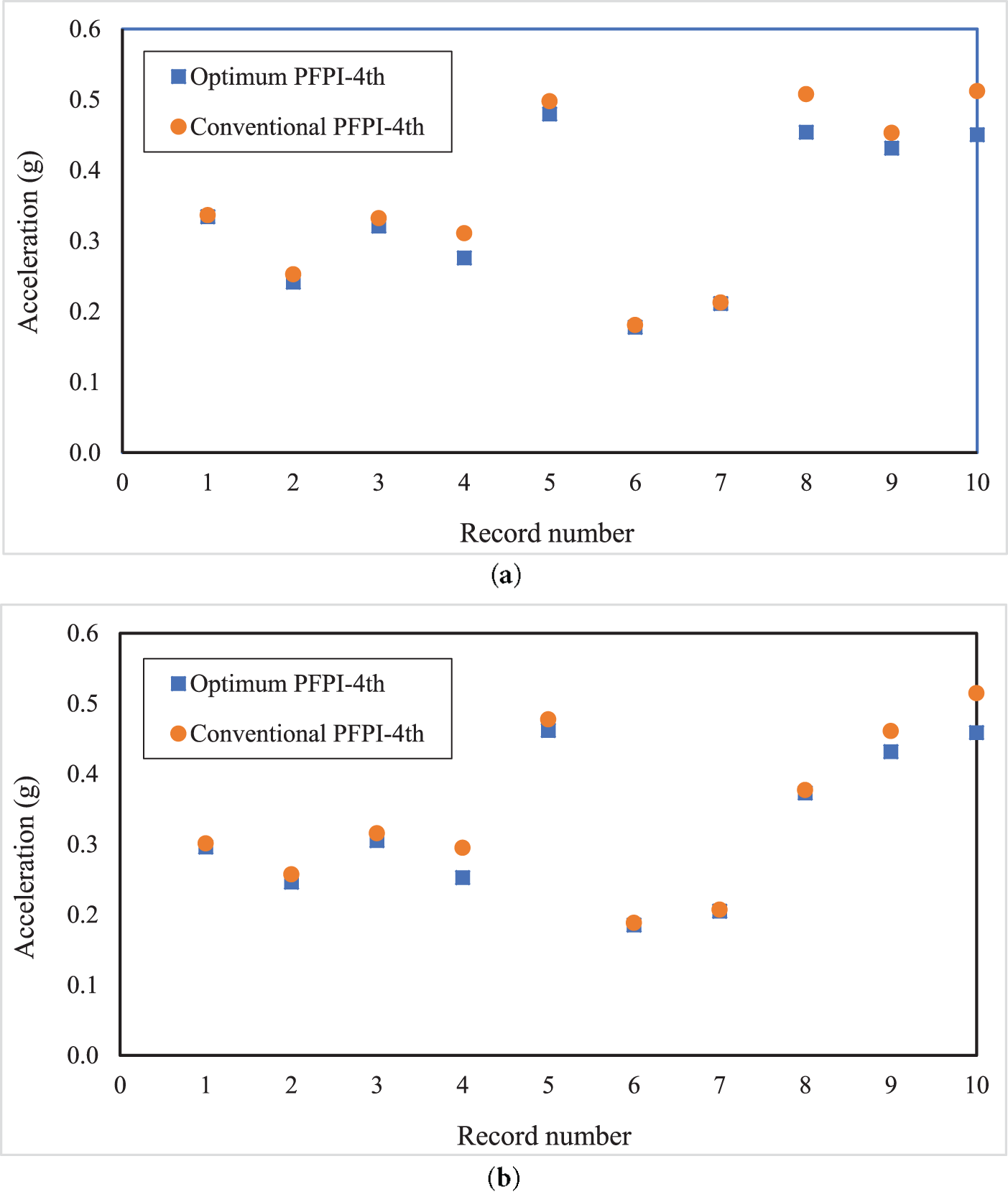
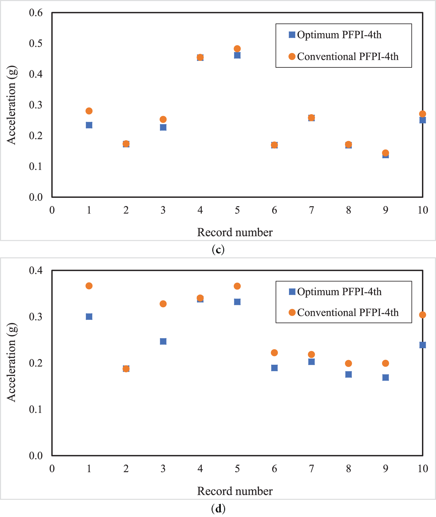
Figure 8: The maximum convective acceleration responses for the optimum and conventional 4th-order PFPIs for different tank geometries and isolation layouts: slender tanks of (a) Model A and (b) Model B; broad tanks of (c) Model A and (d) Model B. The results are drawn for the tanks subjected to long-period ground motions.

The results consistently demonstrate the effectiveness of optimized isolators in reducing convective acceleration. Furthermore, Model A configurations exhibit improved acceleration control relative to Model B. This trend underscores the critical importance of isolator placement in maximizing seismic mitigation. Additionally, slender tanks generally exhibit higher convective acceleration due to their taller geometry and higher convective mode frequencies; however, the relative effectiveness of the optimized isolators remains evident.

8.4 Fragility Curves

To evaluate the seismic vulnerability of isolated elevated tanks under long-period ground motions, IDA was implemented to assess the vulnerability in terms of isolators’ maximum displacement. The fragility curves illustrate the probability of exceedance of critical performance limits as a function of spectral acceleration, Sa. These results offer insight into the effectiveness of each isolation system in reducing structural vulnerability while considering the associated displacement demands. Figs. 9 and 10 illustrate the fragility curves for both PFPI isolators under both Model A and Model B configurations, for broad and slender tanks. In the adopted IDA procedure, each ground motion record is incrementally scaled to increasing levels of spectral acceleration corresponding to the effective isolation period, and nonlinear time-history analyses are performed at each intensity level. The selected engineering demand parameter (EDP) is the maximum isolator displacement, which directly governs the seismic performance of friction pendulum–based isolation systems. For each scaled analysis, the peak displacement demand is extracted and statistically related to the corresponding spectral acceleration, thereby establishing the demand–intensity relationship that underpins the fragility formulation. The resulting fragility curves therefore represent the conditional probability of exceeding predefined displacement-based performance limits at increasing Sa levels.

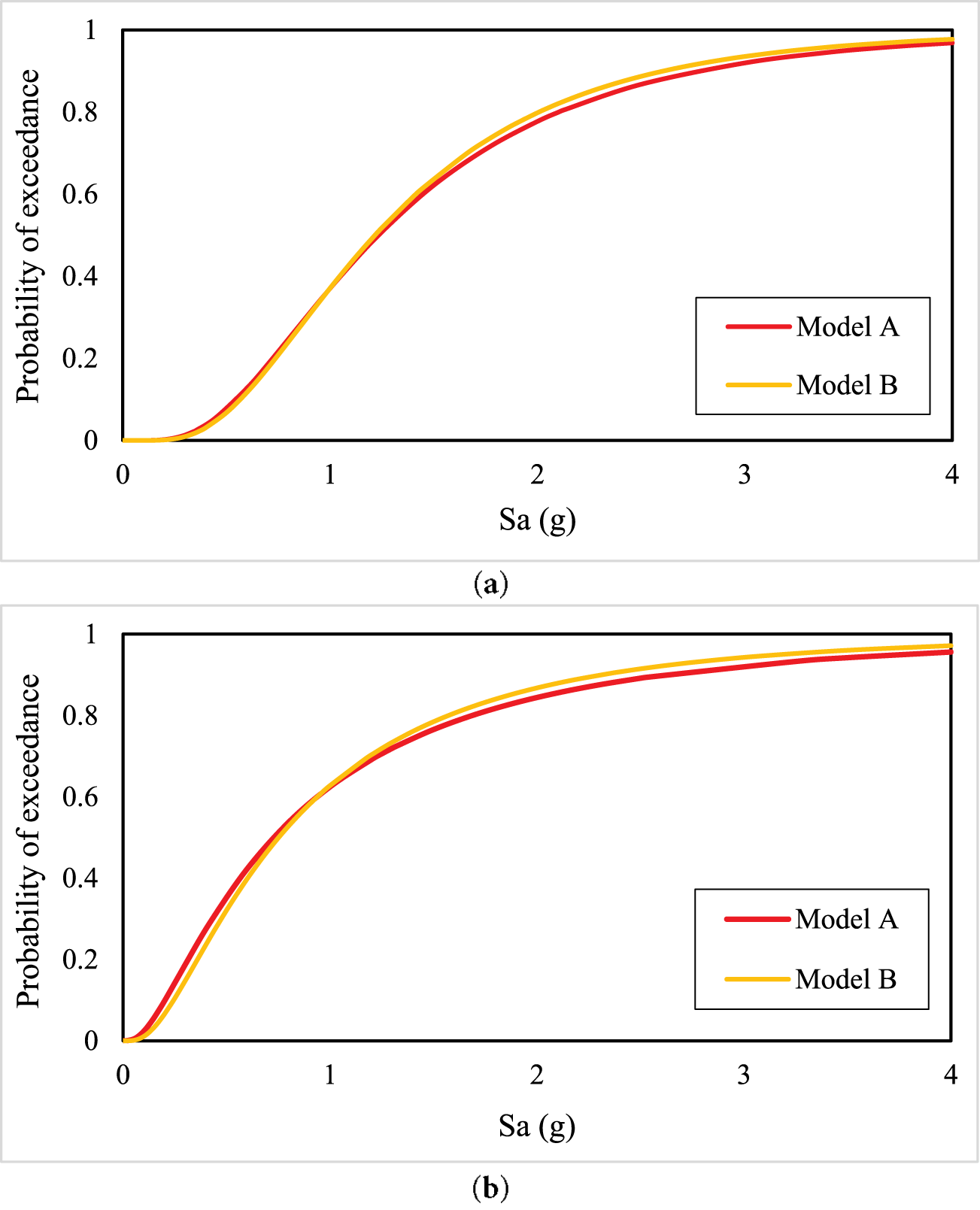
Figure 9: Fragility curves for the optimized 6th-order PFPI isolators utilized in (a) slender and (b) broad tanks.

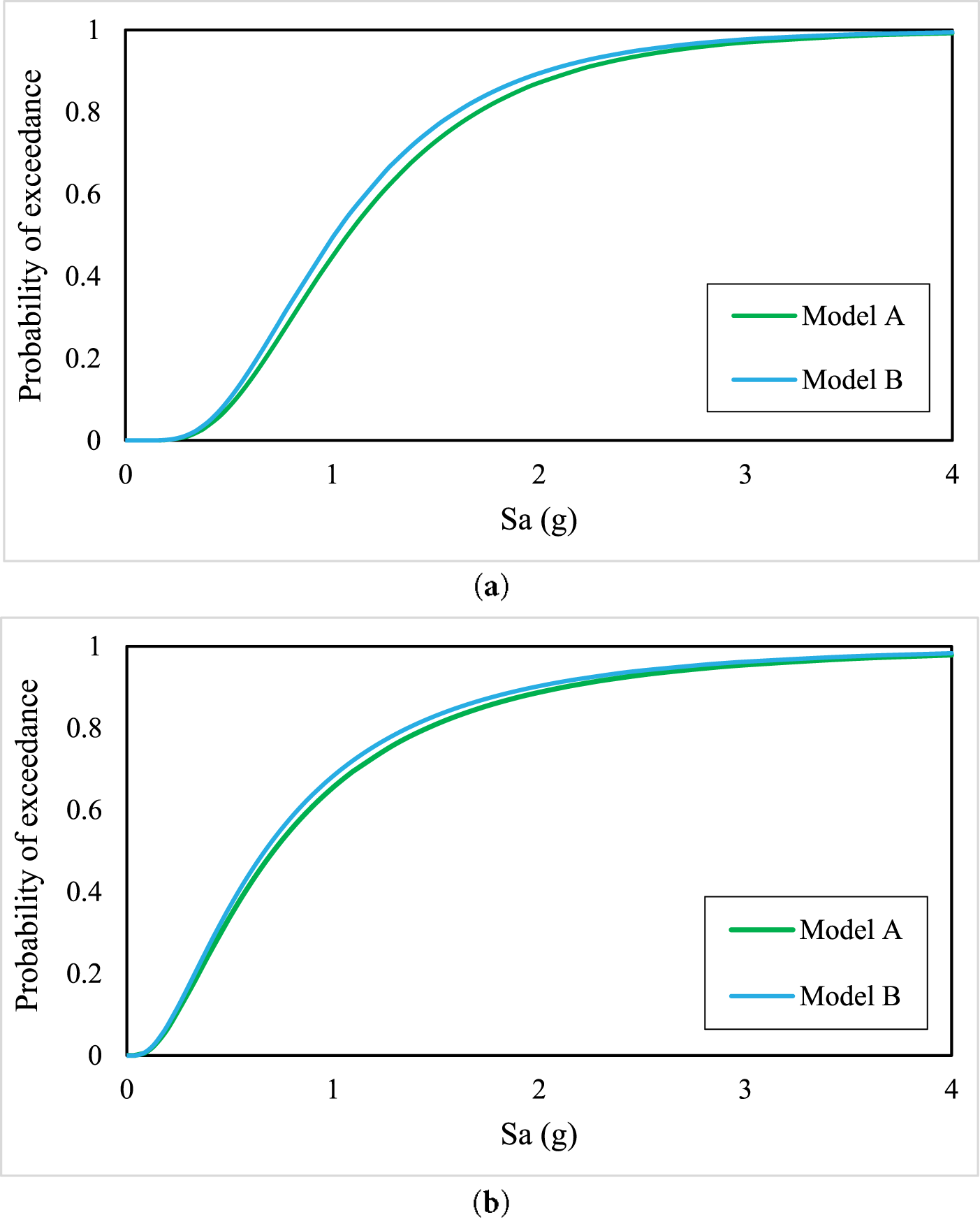
Figure 10: Fragility curves for the optimized 4th-order PFPI isolators utilized in (a) slender and (b) broad tanks.

The performance levels represented by the fragility curves are explicitly defined in terms of threshold values of the maximum isolator displacement, which correspond to distinct limit states associated with increasing response severity. These criteria provide a physically meaningful basis for interpreting the fragility results, ranging from acceptable isolator response to more critical performance conditions. By expressing seismic vulnerability in terms of exceedance probabilities of clearly defined displacement-based limit states, the adopted framework enables a transparent and consistent comparison of the seismic performance of different PFPI configurations and tank geometries under identical hazard conditions.

The fragility curves indicate that broad tanks exhibit a slightly higher probability of exceedance across all considered limit states than slender tanks, suggesting greater vulnerability to seismic demands. Regarding structural safety, Model B consistently yields lower probabilities of exceedance than Model A. This implies that positioning the isolation system closer to the liquid mass is more effective at stabilizing critical displacement parameters, thereby enhancing the elevated tank’s seismic resilience and reducing its overall fragility.

The 6th-order PFPI isolator demonstrates further improvements in fragility performance compared to the 4th-order PFPI isolator. The fragility curves for both broad and slender tanks in Model B display the lowest probability of exceedance at all Sa levels. The difference between Model A and Model B remains, but is less significant than the 4th-order PFPI isolator indicates that increasing the PFPI order enhances seismic resilience regardless of isolator placement. Note that the polynomial degree does not alter the overall behavioral trend of the PFPI response; however, it produces measurable quantitative differences in exceedance probabilities and response levels, as observed in both the broad and slender tank results.

8.5 Hysteretic Force–Displacement Response

The hysteretic force–displacement responses of the optimized PFPI isolators are illustrated in Figs. 11 and 12 for the broad tank configurations subjected to the NS component of the Northridge-01 ground motion. The results demonstrate stable, repeatable hysteresis loops for both the 4th- and 6th-order PFPI models, indicating reliable energy dissipation and the absence of strength or stiffness degradation across loading cycles. A comparison between the PFPI-4th and PFPI-6th configurations indicates that both isolator types provide similar overall hysteretic characteristics, with bounded force levels and smooth transition between loading and unloading phases. Minor differences in loop shape and slope are observed, reflecting the influence of the polynomial order on the displacement-dependent curvature of the sliding surface. For both Model-A and Model-B, the 6th-order PFPI isolator exhibits smoother, more symmetric hysteresis loops, indicating a more gradual stiffness evolution over the displacement range. This behavior is associated with improved control of restoring force at larger displacements, which is consistent with the lower exceedance probabilities and reduced structural response levels observed in the probabilistic analyses. In contrast, the 4th-order PFPI isolator shows slightly steeper force–displacement trajectories, resulting in marginally higher restoring forces at comparable displacement amplitudes. However, these differences do not lead to significant variation in global seismic performance, which is consistent with the comparable objective function values reported in the optimization results. The 6th-order PFPI generally improves seismic performance by reducing force demand and enhancing energy dissipation efficiency, while the 4th-order PFPI may reduce isolator displacement demand in certain cases.

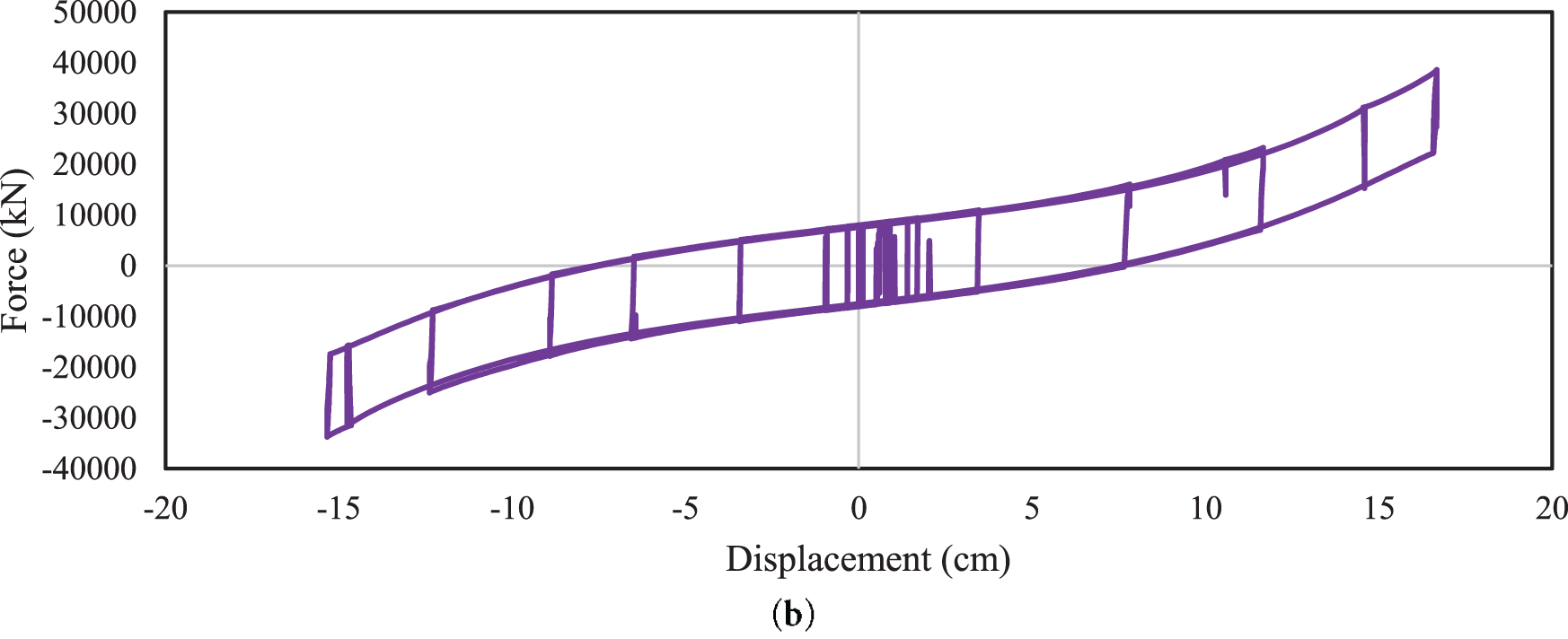
Figure 11: Hysteretic force–displacement response of the base-isolated broad tank (Model-A) equipped with (a) the optimized PFPI-6th isolator, and (b) the optimized PFPI-4th isolator, subjected to the NS component of the Northridge-01 earthquake (RSN = 982).

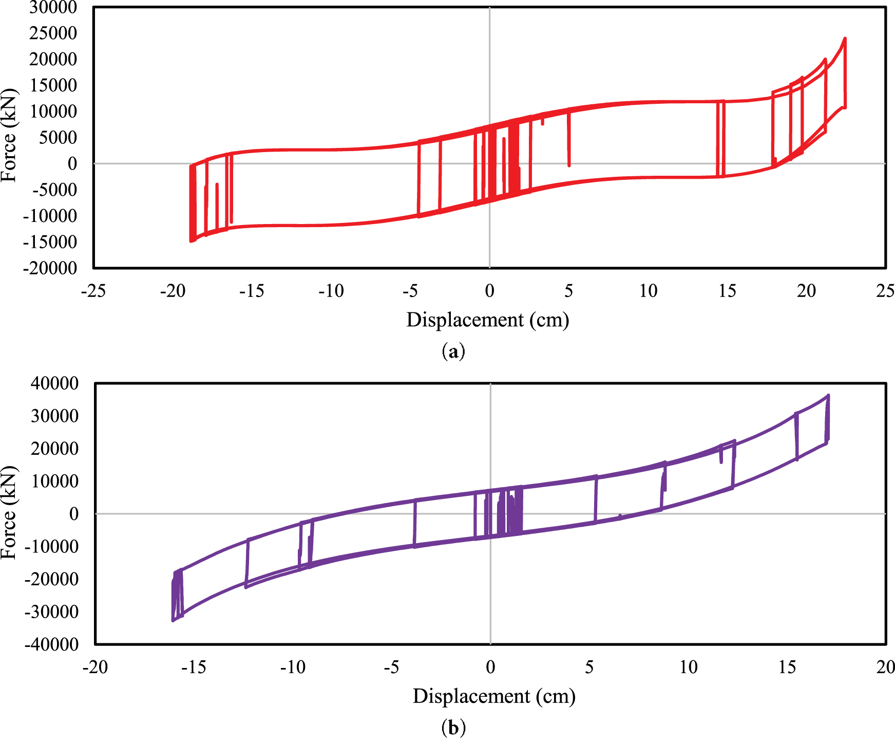
Figure 12: Hysteretic force–displacement response of the base-isolated broad tank (Model-B) equipped with (a) the optimized PFPI-6th isolator, and (b) the optimized PFPI-4th isolator, subjected to the NS component of the Northridge-01 earthquake (RSN = 982).

In both isolation layouts, the hysteretic response exhibits controlled force-softening behavior at larger displacements, corresponding to the intentional reduction in effective stiffness as displacement increases. This response mechanism limits force transmission to the superstructure while allowing the isolator to accommodate the required displacement demand within acceptable design limits.

9  Conclusions

This study presented an integrated approach to enhancing the seismic resilience of elevated liquid storage tanks subjected to long-period ground motions by designing and evaluating curvature-optimized base isolation systems. The research began by applying two optimization algorithms, CS and BSA, to determine the optimal geometric parameters for two isolator types: 6th-order and 4th-order PFPIs. These optimized isolators were then implemented in dynamic models of slender and broad tanks under two isolation configurations: Model A and Model B. The seismic performance was assessed through IDA to evaluate convective acceleration response, followed by fragility analyses to investigate vulnerability based on isolator displacement demand. The following conclusions can be drawn from the present study:

•   Both optimization algorithms, CS and BSA, successfully identified optimal isolator parameters that satisfied nonlinear constraints. CS demonstrated the best performance in terms of convergence speed and stability across all isolator types. Despite different combinations of design variables, the final objective function values across the algorithms were nearly identical, highlighting the robustness of the solution space.

•   The results indicate that, in both configurations, the PFPIs significantly reduce the acceleration transmitted to the tank while accommodating the majority of the seismic displacement at the isolation interface. However, due to differences in mass distribution and stiffness between the two models, the relative balance between displacement demand and acceleration reduction varies. This comparison demonstrates that while the isolation mechanism is effective in both cases, the optimal performance of the PFPI system depends on the dynamic properties of the supported structure, emphasizing the importance of model-specific optimization. The 6th-order PFPI showed the most substantial reduction in peak convective acceleration, achieving up to a 55% decrease compared to the conventional PFPI in slender tanks under Model A configuration. The 4th-order PFPI also improved response performance, though with smaller reductions.

•   The noticeable differences between the optimized parameters of the 4th-order and 6th-order polynomial isolators arise directly from their distinct geometric characteristics. The higher-order polynomial introduces additional flexibility in shaping the sliding surface curvature, allowing a more flexible variation of stiffness and frequency with displacement. As a result, the 6th-order PFPI can achieve stronger stiffness softening at moderate displacements and enhanced stiffness hardening at larger displacements compared to the 4th-order PFPI.

•   Model A configurations outperform Model B in the majority of cases. This outcome reinforces the effectiveness of installing the isolator at the base of the tower, where it directly decouples seismic energy. Slender tanks showed higher absolute acceleration responses than broad tanks due to their higher convective frequencies, but the relative benefit of optimized isolation was significant in both cases.

•   The 6th-order PFPI demonstrated the most favorable fragility characteristics, with the lower probability of exceedance across all spectral acceleration levels, especially in Model B. The 4th-order PFPI performed moderately well in this regard, balancing energy dissipation and displacement control.

•   The combination of optimization algorithms and performance-based seismic assessment offers a powerful tool for designing high-performance isolation systems. Curvature-optimized isolators, particularly the 6th-order PFPI, can significantly enhance both dynamic response mitigation and seismic safety.

•   The hysteretic force–displacement responses confirmed stable and repeatable nonlinear behavior for both 4th- and 6th-order PFPI isolators, indicating reliable energy dissipation without stiffness or strength degradation under strong ground motion. While both formulations exhibited similar qualitative hysteretic characteristics, the 6th-order PFPI generally produced smoother force evolution and improved performance consistency, consistent with the probabilistic response trends observed in the study.

•   The results indicate that while conventional friction pendulum isolators remain suitable for low- to moderate-seismic regions, optimized variable-curvature friction pendulum isolators provide superior performance for elevated liquid storage tanks subjected to long-period and high-intensity ground motions. In other words, the application of variable-curvature friction pendulum isolators is not intended to replace conventional friction pendulum isolators in all seismic regions. In areas of low to moderate seismicity, where ground motions are predominantly short-period, conventional Frequency Pendulum Isolators (FPIs) with fixed curvature can provide adequate seismic protection. However, in high-seismicity regions or sites characterized by long-period or near-fault ground motions, the constant natural period of FPIs may lead to resonance effects and amplified structural response. In such cases, VFPIs offer a significant advantage by adaptively modifying their effective stiffness and isolation frequency as the excitation intensity increases. Therefore, the proposed system is particularly suited for regions with high seismic demand and long-period ground motion characteristics.

Although the results of this study seem promising, other types of FPSs, combined with other metaheuristic algorithms, should be further examined to achieve a more comprehensive outcome. These are currently followed by the authors and will be disseminated in the future.

Acknowledgement: Not applicable.

Funding Statement: The authors received no specific funding for this study.

Author Contributions: The authors confirm contribution to the paper as follows: Conceptualization, Mojgan Mohammadi and Naser Khaji; methodology, Mojgan Mohammadi and Naser Khaji; software, Mojgan Mohammadi; validation, Mojgan Mohammadi and Naser Khaji; formal analysis, Mojgan Mohammadi; investigation, Mojgan Mohammadi; resources, Mojgan Mohammadi and Naser Khaji; data curation, Mojgan Mohammadi; writing—original draft preparation, Mojgan Mohammadi; writing—review and editing, Mojgan Mohammadi and Naser Khaji; visualization, Mojgan Mohammadi and Naser Khaji; supervision, Naser Khaji; project administration, Naser Khaji. All authors reviewed and approved the final version of the manuscript.

Availability of Data and Materials: The data that support the findings of this study are available from the Corresponding Author, Naser Khaji, upon reasonable request.

Ethics Approval: Not applicable.

Conflicts of Interest: The authors declare no conflicts of interest.

References

1. Gates W. Elevated and ground-supported steel storage tanks. Reconnaissance Report, Imperial County, California Earthquake of October 15, 1979. Oakland, CA, USA: Earthquake Engineering Research Institute; 1980. [Google Scholar]

2. Knoy CE. Performance of elevated tanks during recent California seismic events. In: AWWA Annual Conference & Exhibition; 1995 Jun 18–22; Anaheim, CA, USA. [Google Scholar]

3. Cooper TW. A study of the performance of petroleum storage tanks during earthquakes, 1933–1995. Gaithersburg, MD, USA: US National Institute of Standards and Technology; 1997. [Google Scholar]

4. Haroun MA. Vibration studies and tests of liquid storage tanks. Earthq Eng Struct Dyn. 1983;11(2):179–206. doi:10.1002/eqe.4290110204. [Google Scholar] [CrossRef]

5. Hamdan FH. Seismic behaviour of cylindrical steel liquid storage tanks. J Constr Steel Res. 2000;53(3):307–33. doi:10.1016/S0143-974X(99)00039-5. [Google Scholar] [CrossRef]

6. Hosseini SEA, Beskhyroun S. Fluid storage tanks: a review on dynamic behaviour modelling, seismic energy-dissipating devices, structural control, and structural health monitoring techniques. Structures. 2023;49(3):537–56. doi:10.1016/j.istruc.2023.01.146. [Google Scholar] [CrossRef]

7. Volikos K, Konstandakopoulou F, Asteris P, Hatzigeorgiou G. Recent advancements in seismic analysis and design of liquid storage tanks. Soil Dyn Earthq Eng. 2025;198(2):109309. doi:10.1016/j.soildyn.2025.109309. [Google Scholar] [CrossRef]

8. Haroun MA, Ellaithy HM. Seismically induced fluid forces on elevated tanks. J Tech Topics. 1985;111(1):1–15. doi:10.1061/jtcedl.0000023. [Google Scholar] [CrossRef]

9. Majdi A, Sadeghi-Movahhed A, Farsangi EN, Mashayekhi M, Almujibah H, De Domenico D. Application of the modified endurance time method for predicting seismic response of base-isolated structures under pounding. J Earthq Tsunami. 2025;19(3):2450037. doi:10.1142/s1793431124500374. [Google Scholar] [CrossRef]

10. Shenton HW, Hampton FP. Seismic response of isolated elevated water tanks. J Struct Eng. 1999;125(9):965–76. doi:10.1061/(asce)0733-9445(1999)125:9(965). [Google Scholar] [CrossRef]

11. Mitra S, Debbarma R. Seismic response mitigation of elevated water storage tank using base isolation system. In: Proceedings of the International Conference on Advances in Structural Mechanics and Applications; 2021 Mar 26–28; Silchar, India. Cham, Switzerland: Springer International Publishing; 2022. p. 338–51. doi:10.1007/978-3-031-05509-6_28. [Google Scholar] [CrossRef]

12. Shrimali MK, Jangid RS. Earthquake response of isolated elevated liquid storage steel tanks. J Constr Steel Res. 2003;59(10):1267–88. doi:10.1016/S0143-974X(03)00066-X. [Google Scholar] [CrossRef]

13. Shrimali MK. Earthquake response of elevated liquid storage tanks isolated by FPS under bi-direction excitation. Adv Vib Eng. 2008;7(4):389–405. [Google Scholar]

14. Seleemah AA, El-Sharkawy M. Seismic analysis and modeling of isolated elevated liquid storage tanks. Earthq Struct. 2011;2(4):397–412. doi:10.12989/eas.2011.2.4.397. [Google Scholar] [CrossRef]

15. Rabiei M, Khoshnoudian F. Seismic response of elevated liquid storage tanks using double concave friction pendulum bearings with tri-linear behavior. Adv Struct Eng. 2013;16(2):315–37. doi:10.1260/1369-4332.16.2.315. [Google Scholar] [CrossRef]

16. Moeindarbari H, Malekzadeh M, Taghikhany T. Probabilistic analysis of seismically isolated elevated liquid storage tank using multi-phase friction bearing. Earthq Struct. 2014;6(1):111–25. doi:10.12989/eas.2014.6.1.111. [Google Scholar] [CrossRef]

17. Paolacci F. On the effectiveness of two isolation systems for the seismic protection of elevated tanks. J Press Vessel Technol. 2015;137(3):31801. doi:10.1115/1.4029590. [Google Scholar] [CrossRef]

18. Moslemi M, Kianoush MR. Application of seismic isolation technique to partially filled conical elevated tanks. Eng Struct. 2016;127(2):663–75. doi:10.1016/j.engstruct.2016.09.009. [Google Scholar] [CrossRef]

19. Barik JR, Biswal KC. Dynamic characteristics of seismically isolated rectangular tank-liquid–block systems implementing lead rubber bearing isolator. J Earthq Tsunami. 2023;17(6):2350027. doi:10.1142/s1793431123500276. [Google Scholar] [CrossRef]

20. Kumar H, Saha SK. Seismic performance of base-isolated elevated liquid storage tanks considering soil-structure interaction. Pract Period Struct Des Constr. 2021;26(1):4020062. doi:10.1061/(asce)sc.1943-5576.0000545. [Google Scholar] [CrossRef]

21. Ghoohestani S, Shekari MR, Zareifard MR, Amiri SM. On the nonlinear seismic response of liquid filled thin-walled steel elevated containers isolated by bearings to earthquake ground motions. Int J Press Vessels Pip. 2022;199(3):104754. doi:10.1016/j.ijpvp.2022.104754. [Google Scholar] [CrossRef]

22. Hashemi S, Aghashiri MH, Ehteshami A, Kianoush R. Seismic isolation effects on elevated and ground-supported flexible concrete cylindrical tanks under bi-directional excitation using an advanced mechanical model. J Earthq Tsunami. 2024;18(3):2450002. doi:10.1142/s1793431124500027. [Google Scholar] [CrossRef]

23. Zayas V, Low SS, Mahin SA. The FPS earthquake resisting system, experimental report. Berkeley, CA, USA: Earthquake Engineering Research Center, College of Engineering, University of California; 1987. Report No.: UCB/EERC-8701. [Google Scholar]

24. Zhang C, Ali A. The advancement of seismic isolation and energy dissipation mechanisms based on friction. Soil Dyn Earthq Eng. 2021;146:106746. doi:10.1016/j.soildyn.2021.106746. [Google Scholar] [CrossRef]

25. Mokha A, Constantinou MC, Reinhorn AM, Zayas VA. Experimental study of friction-pendulum isolation system. J Struct Eng. 1991;117(4):1201–17. doi:10.1061/(asce)0733-9445(1991)117:4(1201). [Google Scholar] [CrossRef]

26. Lu LY, Wang J, Hsu CC. Sliding isolation using variable frequency bearings for near-fault ground motions. In: Proceedings of the 4th International Conference on Earthquake Engineering; 2006 Oct 12–13; Taipei, Taiwan. [Google Scholar]

27. Panchal VR, Jangid RS. Behaviour of liquid storage tanks with VCFPS under near-fault ground motions. Struct Infrastruct Eng. 2012;8(1):71–88. doi:10.1080/15732470903300919. [Google Scholar] [CrossRef]

28. Panchal VR, Jangid RS. Seismic response of liquid storage steel tanks with variable frequency pendulum isolator. KSCE J Civ Eng. 2011;15(6):1041–55. doi:10.1007/s12205-011-0945-y. [Google Scholar] [CrossRef]

29. Pranesh M, Sinha R. VFPI: an isolation device for aseismic design. Earthq Eng Struct Dyn. 2000;29(5):603–27. doi:10.1002/(sici)1096-9845(200005)29:5<603::aid-eqe927>3.0.co;2-w. [Google Scholar] [CrossRef]

30. Saha A, Saha P, Patro SK. Polynomial friction pendulum isolators (PFPIs) for seismic performance control of benchmark highway bridge. Earthq Eng Eng Vib. 2017;16(4):827–40. doi:10.1007/s11803-017-0418-5. [Google Scholar] [CrossRef]

31. Darvishi R, Abdollahzadeh G. Cyclic behaviour of triple friction pendulum isolators with elliptical surfaces. Proc Inst Civ Eng Struct Build. 2021;174(3):225–35. doi:10.1680/jstbu.18.00186. [Google Scholar] [CrossRef]

32. Admane HA, Murnal P. Comparative analysis of SIVC systems using simplified analytical modeling for practical design. Pract Period Struct Des Constr. 2021;26(1):4020051. doi:10.1061/(asce)sc.1943-5576.0000536. [Google Scholar] [CrossRef]

33. Sheikh H, Van Engelen NC, Ruparathna R. A review of base isolation systems with adaptive characteristics. Structures. 2022;38(5):1542–55. doi:10.1016/j.istruc.2022.02.067. [Google Scholar] [CrossRef]

34. Lu LY, Lee TY, Yeh SW. Theory and experimental study for sliding isolators with variable curvature. Earthq Eng Struct Dyn. 2011;40(14):1609–27. doi:10.1002/eqe.1106. [Google Scholar] [CrossRef]

35. Shaikhzadeh AA, Karamoddin A. Effectiveness of sliding isolators with variable curvature in near-fault ground motions. Struct Des Tall Spec Build. 2016;25(6):278–96. doi:10.1002/tal.1258. [Google Scholar] [CrossRef]

36. Zheng W, Tan P, Li J, Wang H, Liu Y, Xian Z. Superelastic pendulum isolator with multi-stage variable curvature for seismic resilience enhancement of cold-regional bridges. Eng Struct. 2023;284(5):115960. doi:10.1016/j.engstruct.2023.115960. [Google Scholar] [CrossRef]

37. Krishnamoorthy A, Bhadania V, Kavyasree M, Prajapati V, Kumar MP. Variable curvature pendulum isolator system for seismic isolation of liquid storage tanks. Innov Infrastruct Solut. 2023;8(11):303. doi:10.1007/s41062-023-01281-9. [Google Scholar] [CrossRef]

38. Wei B, Yang Z, Xiao B, Jiang L, Yu Y. Simplified design theory of variable curvature friction pendulum bearing with adaptive capability and its application in railway bridge. Structures. 2024;63:106370. doi:10.1016/j.istruc.2024.106370. [Google Scholar] [CrossRef]

39. Lu LY, Ramadhanti NN, Lee TY. Multiple performance objective design for a sliding isolator with variable curvature. Eng Struct. 2024;307(3):117815. doi:10.1016/j.engstruct.2024.117815. [Google Scholar] [CrossRef]

40. Nigdeli SM, Bekdaş G, Alhan C. Optimization of seismic isolation systems via harmony search. Eng Optim. 2014;46(11):1553–69. doi:10.1080/0305215X.2013.854352. [Google Scholar] [CrossRef]

41. Ocak A, Nigdeli SM, Bekdaş G, Kim S, Geem ZW. Optimization of seismic base isolation system using adaptive harmony search algorithm. Sustainability. 2022;14(12):7456. doi:10.3390/su14127456. [Google Scholar] [CrossRef]

42. Tsipianitis A, Tsompanakis Y. Optimizing the seismic response of base-isolated liquid storage tanks using swarm intelligence algorithms. Comput Struct. 2021;243(4):106407. doi:10.1016/j.compstruc.2020.106407. [Google Scholar] [CrossRef]

43. Tsipianitis A, Spachis A, Tsompanakis Y. Combined optimization of friction-based isolators in liquid storage tanks. Appl Sci. 2022;12(19):9879. doi:10.3390/app12199879. [Google Scholar] [CrossRef]

44. Liang Y, Kong YZ, Zhao CX, Liu RQ, Luo J, Zhu RH. Time-varying seismic fragility analysis of ECC-RC composite bridge with high-strength steel bars. J Earthq Tsunami. 2024;18(01):2350029. doi:10.1142/s179343112350029x. [Google Scholar] [CrossRef]

45. Zhang Y, Shi Y, Sun B, Wang Z. Estimation of aleatory randomness by Sa(T1)-based intensity measures in fragility analysis of reinforced concrete frame structures. Comput Model Eng Sci. 2022;130(1):74–96. doi:10.32604/cmes.2022.016857. [Google Scholar] [CrossRef]

46. Jough FKG. Fuzzy logic-based fragility curve development for steel moment-resisting frames considering uncertainties in seismic response. J Earthq Tsunami. 2024;18(5):2450014. doi:10.1142/s1793431124500143. [Google Scholar] [CrossRef]

47. Sun B, Zhang Y, Huang C. Machine learning-based seismic fragility analysis of large-scale steel buckling restrained brace frames. Comput Model Eng Sci. 2020;125(2):755–76. doi:10.32604/cmes.2020.09632. [Google Scholar] [CrossRef]

48. Wang M, Sun Z, Sun J, Cui L, Wu Y. Probabilistic seismic fragility assessment of vertical storage tank with a floating roof. Structures. 2023;48:318–30. doi:10.1016/j.istruc.2022.12.104. [Google Scholar] [CrossRef]

49. Tsipianitis A, Tsompanakis Y. Seismic vulnerability assessment of liquid storage tanks isolated by sliding-based systems. Adv Civ Eng. 2018;2018(1):5304245. doi:10.1155/2018/5304245. [Google Scholar] [CrossRef]

50. Zhao Z, Lu X, Guo Y, Zhao X. Seismic fragility assessment of base-isolated steel water storage tank. Shock Vib. 2020;2020(1):8835943. doi:10.1155/2020/8835943. [Google Scholar] [CrossRef]

51. Shrimali MK, Jangid RS. Seismic response of liquid storage tanks isolated by sliding bearings. Eng Struct. 2002;24(7):909–21. doi:10.1016/S0141-0296(02)00009-3. [Google Scholar] [CrossRef]

52. Ahmadi A, Khaji N, Bazrafshan A. Seismic analysis of base-isolated liquid storage tanks incorporating a new probabilistic long-period critical excitation method. Results Eng. 2025;26(5):104977. doi:10.1016/j.rineng.2025.104977. [Google Scholar] [CrossRef]

53. Wang YP, Liao WH, Lee CL. A state-space approach for dynamic analysis of sliding structures. Eng Struct. 2001;23(7):790–801. doi:10.1016/S0141-0296(00)00096-1. [Google Scholar] [CrossRef]

54. Yang XS, Deb S. Cuckoo search via Lévy flights. In: Proceedings of the 2009 World Congress on Nature & Biologically Inspired Computing (NaBIC); 2009 Dec 9–11; Coimbatore, India. p. 210–4. doi:10.1109/NABIC.2009.5393690. [Google Scholar] [CrossRef]

55. Meng XB, Gao XZ, Lu L, Liu Y, Zhang H. A new bio-inspired optimisation algorithm: bird swarm algorithm. J Exp Theor Artif Intell. 2016;28(4):673–87. doi:10.1080/0952813x.2015.1042530. [Google Scholar] [CrossRef]

56. Lu LY, Lee TY, Juang SY, Yeh SW. Polynomial friction pendulum isolators (PFPIs) for building floor isolation: an experimental and theoretical study. Eng Struct. 2013;56(1):970–82. doi:10.1016/j.engstruct.2013.06.016. [Google Scholar] [CrossRef]

57. Koketsu K, Miyake H. A seismological overview of long-period ground motion. J Seismol. 2008;12(2):133–43. doi:10.1007/s10950-007-9080-0. [Google Scholar] [CrossRef]

58. Zhou Y, Ping T, Gong S, Zhu Y. An improved defining parameter for long-period ground motions with application of a super-tall building. Soil Dyn Earthq Eng. 2018;113(2):462–72. doi:10.1016/j.soildyn.2018.06.018. [Google Scholar] [CrossRef]