
 Submit a Paper
 Propose a Special lssue
 Open Access
ARTICLE

Optimal Resource Allocation in a Bacterial Growth Model Under Cold Stress and Temperature
Tandy School of Computer Science, University of Tulsa, Tulsa, OK, USA
* Corresponding Authors: Saira Batool. Email: ; Muhammad Imran. Email:
; Brett McKinney. Email:
(This article belongs to the Special Issue: Advances in Mathematical Modeling: Numerical Approaches and Simulation for Computational Biology)
Computer Modeling in Engineering & Sciences 2026, 146(3), 30 https://doi.org/10.32604/cmes.2026.079067
Received 14 January 2026; Accepted 03 March 2026; Issue published 30 March 2026
 View Full Text
 Download PDF
Abstract
Bacterial growth requires strategic allocation of limited intracellular resources, especially under cold stress, where stabilized messenger ribonucleic acid (mRNA) secondary structures slow translation by impairing ribosome binding. Escherichia coli (E. coli) counters this bottleneck by inducing the cold-shock protein A (CspA), an RNA chaperone that remodels inhibitory structures. However, synthesizing CspA diverts biosynthetic capacity from ribosome production and metabolism, creating a fundamental resource-allocation trade-off. In this work, we develop a dynamical model capturing the interplay between metabolic precursors, ribosomes, and CspA, and use it to examine how growth and allocation patterns shift with temperature. Steady-state analysis shows that each temperature produces a distinct, locally stable equilibrium, illustrating how cold environments reshape cellular priorities. We then formulate growth maximization as an optimal control problem, solved using Pontryagin’s Maximum Principle, to identify allocation strategies that balance translation maintenance and biomass production. The resulting optimal strategies exhibit bang-bang and singular structures, highlighting periods of extreme and intermediate allocation that reflect how bacteria might dynamically prioritize competing cellular functions. These control patterns converge to their corresponding steady state allocations and provide quantitative insight into optimal resource management under cold stress. These results provide a quantitative optimal-control framework linking RNA-level cold-shock adaptation to proteome allocation and growth, yielding testable predictions for how bacteria balance translational maintenance and biomass production at suboptimal temperatures.Keywords
Microorganisms are constantly exposed to fluctuations in their environment, particularly in nutrient availability and temperature. To survive and thrive under such conditions, they have evolved sophisticated strategies that enable dynamic physiological adaptation [1]. This adaptation is primarily achieved through large-scale reorganization of gene expression, including regulation of genes responsible for nutrient uptake, energy production, protein synthesis, and stress responses [2,3]. Central to this process is the efficient allocation of cellular resources, particularly protein synthesis capacity, across competing functional demands [4–6]. Among environmental variables, temperature is especially influential, directly affecting reaction kinetics, enzyme activity, and the stability of cellular structures [7]. Under cold stress, biochemical reactions slow markedly, and energy availability becomes limited, intensifying the challenge of maintaining balanced resource allocation [1].
Exposure to low temperatures triggers extensive physiological reorganization, including the redistribution of limited resources such as ribosomes, metabolic enzymes, and energy toward essential survival functions. In these conditions, messenger RNA (mRNA) molecules tend to form stable secondary structures, such as hairpins, that impede ribosome binding and slow translation, thereby reducing protein synthesis efficiency [1]. To overcome these obstacles, Escherichia coli induces cold-adaptive proteins (CSPs), particularly CspA, which is rapidly upregulated under low temperatures and can constitute up to 10% of total cellular protein, reaching intracellular concentrations around 100 μM [8–10]. Acting as RNA chaperones, CSPs destabilize inhibitory secondary structures in nucleic acids, facilitating efficient transcription and translation during cold adaptation and thereby restoring cellular homeostasis under low-temperature conditions.
CspA functions primarily as an RNA chaperone, binding transiently to single-stranded regions of mRNA with low sequence specificity and moderate affinity [8,11]. It binds cooperatively to single-stranded RNA stretches longer than 74 nucleotides, with a minimal concentration of approximately
Experimental studies indicate that low temperatures reduce translation efficiency due to stabilization of mRNA secondary structures, limiting protein synthesis and growth. To cope with this challenge, E. coli induces cold-shock protein CspA, which alleviates inhibitory RNA structures [9,12]. However, the synthesis of CspA consumes significant cellular resources, creating a trade-off. Excessive CspA production competes with ribosome biogenesis and other essential processes, potentially limiting overall growth. This suggests the existence of an optimal CspA level that balances the benefits of enhanced translation against the costs of resource allocation, providing a natural framework for applying optimal control theory to quantify growth strategies under cold-shock conditions. Optimal control provides a theoretical benchmark for quantifying such growth strategies under cold-shock conditions [13,14], and although exact optimal strategies are unlikely to be implemented physiologically, they represent a gold standard that can be used to evaluate how closely real bacterial regulatory mechanisms approximate optimal resource allocation.
Microbial growth and resource allocation have been extensively investigated from both experimental and theoretical perspectives [7,13,14]. Early systems-biology studies established empirical growth laws linking ribosome content, proteome partitioning, and cellular growth rate, revealing fundamental trade-offs in bacterial resource economics [15–17]. Building on these biological insights, several theoretical frameworks have sought to formalize microbial growth optimization using mathematical and control-theoretic approaches. For instance, Giuliodori et al. [12] formulated microbial growth in fluctuating environments as an optimal control problem, while Yegorov et al. [13,14] extended this work to include protein degradation, recycling, and temperature-dependent kinetics. More recently, Mairet et al. examined proteome allocation under temperature stress, showing that extreme conditions redirect resources to chaperone-mediated repair processes [18]. Despite these advances, quantitative models that specifically capture low-temperature adaptation and its associated trade-offs in Escherichia coli remain limited. Addressing this gap, the present study develops a dynamical model to investigate how bacteria allocate limited translational resources to balance growth and stress adaptation under cold-shock conditions.
Building on these principles, we formulate a dynamical model of E. coli under low temperature using ordinary differential equations (ODEs) to describe the interplay between ribosomes, metabolism, and CspA. The RNA-chaperone activity of CspA is represented by a modulation factor applied to the effective protein-synthesis rate, reflecting its role in alleviating inhibitory mRNA secondary structures. To focus on the primary trade-off between translation efficiency and ribosomal availability, we assume that other regulatory factors and stress responses not directly related to ribosome or CspA allocation are negligible. For the purpose of this model, we assume that CspA-mediated translation is the main mechanism driving adaptation under low temperatures. Under these assumptions, ribosome and CspA synthesis are dynamically regulated to maximize cumulative growth, defined as the total increase in cellular components (ribosomes, CspA, and metabolic intermediates), over a defined time horizon. Resource allocation is formulated as a dynamic optimal control problem in which the objective is to maximize cumulative cellular growth over a defined time horizon. In this framework, the control variables represent the fractional distribution of translational resources between ribosome synthesis and CspA production. Applying Pontryagin’s Maximum Principle yields the necessary conditions for optimal resource allocation and enables the identification of candidate strategies that balance growth with stress adaptation. This formulation supports the analysis of both open-loop and feedback control policies, offering insights into how temporal dynamics and environmental conditions shape optimal bacterial growth trajectories under cold-shock stress.
Overall, this study introduces a quantitative framework that integrates molecular cold-shock mechanisms with optimal resource allocation principles. By explicitly linking RNA-level adaptation to proteome allocation and growth optimization, the model offers new insight into how E. coli balances translational efficiency and biomass production at suboptimal temperatures. The results generate testable predictions for cold-shock adaptation and provide a foundation for future experimental and theoretical investigations into microbial growth strategies under low-temperature stress. The paper is organized as follows. Section 2 outlines the mathematical framework governing the dynamical model. Section 3 analyzes temperature-dependent steady states and stability. Section 4 introduces the optimal control problem and characterizes optimal allocation strategies. Section 5 presents the key conclusions and highlights potential directions for future research.
Consider a population of self-replicating prokaryotic cells, such as Escherichia coli, in a continuous stirred-tank reactor (CSTR) of constant volume. Let P, M, R, and C [g] denote the total masses of precursor metabolites (amino acids), metabolic machinery (enzymes involved in the uptake and conversion of nutrients into precursors), gene expression machinery (polymerases and ribosomes), and the cold-shock protein CspA, respectively. The metabolic machinery converts external substrates into precursors, while the gene-expression machinery and CspA utilize these precursors to synthesize the macromolecules required for cellular growth and maintenance. A schematic diagram (Fig. 1) illustrates the mass fluxes and catalytic interactions within the system. Based on the mass balances of these components, the system dynamics are described by a controlled set of ordinary differential equations (ODEs) that capture the time evolution of precursors, metabolic enzymes, ribosomes, and CspA (Eq. (1)). Unlike classical microbial growth models in which translational efficiency is prescribed as a fixed or externally scaled parameter, the present formulation treats translation as an endogenous, state-dependent process modulated by the intracellular concentration of the cold-shock protein CspA.
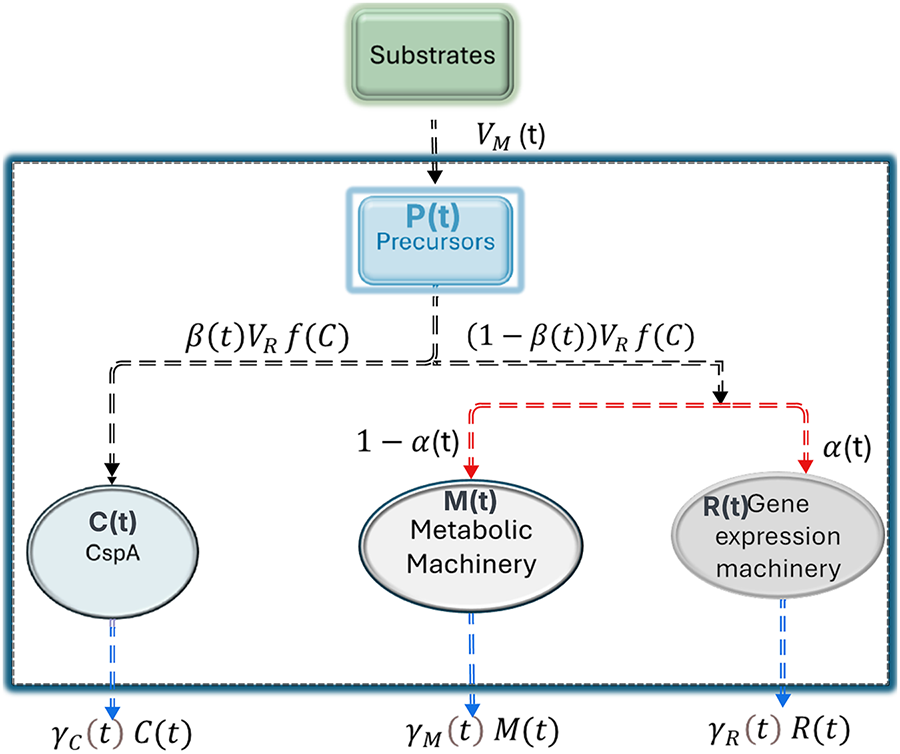
Figure 1: Flow diagram represents the flow or distribution of nutrients between different parts of the cellular machinery.
with following initial conditions,
where
•
•
•
•
•
• Cells in the population are assumed to share a constant cytoplasmic density, with
• The structural volume of the cell population is defined as
representing the volume occupied by the macromolecules of the metabolic and gene expression machinery and cspA, excluding monomeric precursors.
• The concentrations of the cellular components are defined as
Using the relation in Eq. (2), we can rewrite it as:
• The growth rate of the self-replicating system is
Now, after the modification as mentioned above, the proposed model (Eq. (1)) can be written as follows:
where the dynamics of
Following the work of [13], the metabolic flux can be described as
where
with
with
where
Now, let us rescale the model to simplify its mathematical analysis. We introduce the following dimensionless variables and constants:
Substituting the nondimensional variables into Eq. (2) yields
The system expressed in terms of concentrations (Eq. (4)) can be transformed into a dimensionless form using the rescaled variables and constants:
with the initial conditions:
where
and
In the scaled system (Eq. (8)), the dynamical expression of
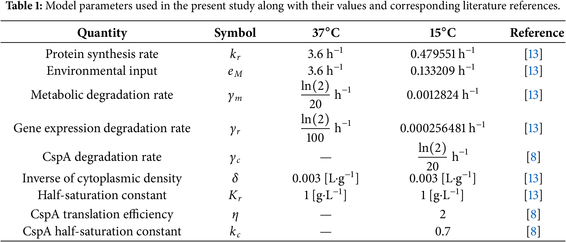
To model bacterial growth and resource allocation under cold-shock conditions, we used kinetic parameters previously measured and validated at 37°C [13]. Because direct experimental data at 15°C are limited, most parameters were adjusted using the
This
Since almost all the parameters of the proposed model (Eq. (4)) depend on the temperature of the environment. Therefore, we analyze the impact of different levels of temperature on the dynamics of the proposed model in this section.
Following the resource allocation framework of Giordano et al. (2016), we determine the steady state
of the system (Eq. (8)), at which the growth rate
The resulting optimal allocation at the reference temperature 15°C is
with an associated growth rate
At this optimum, the proteome fractions are distributed as
where
The convergence of the dynamical system towards the steady state shows that
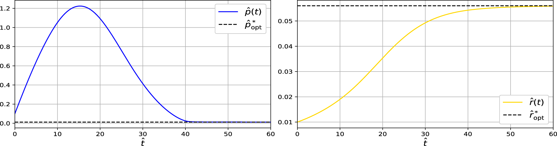
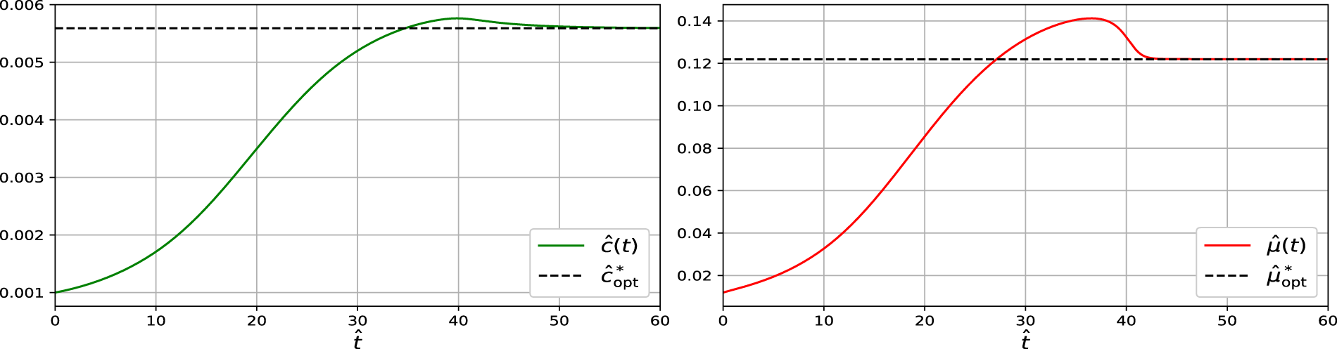
Figure 2: Simulation of the dynamical system showing convergence of
In addition to the reference case at
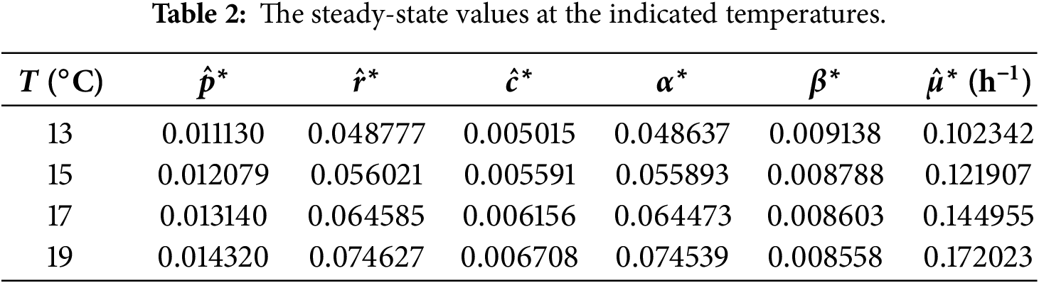
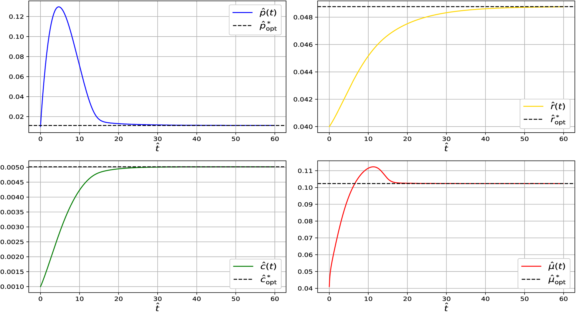
Figure 3: Simulation of the dynamical system showing convergence of
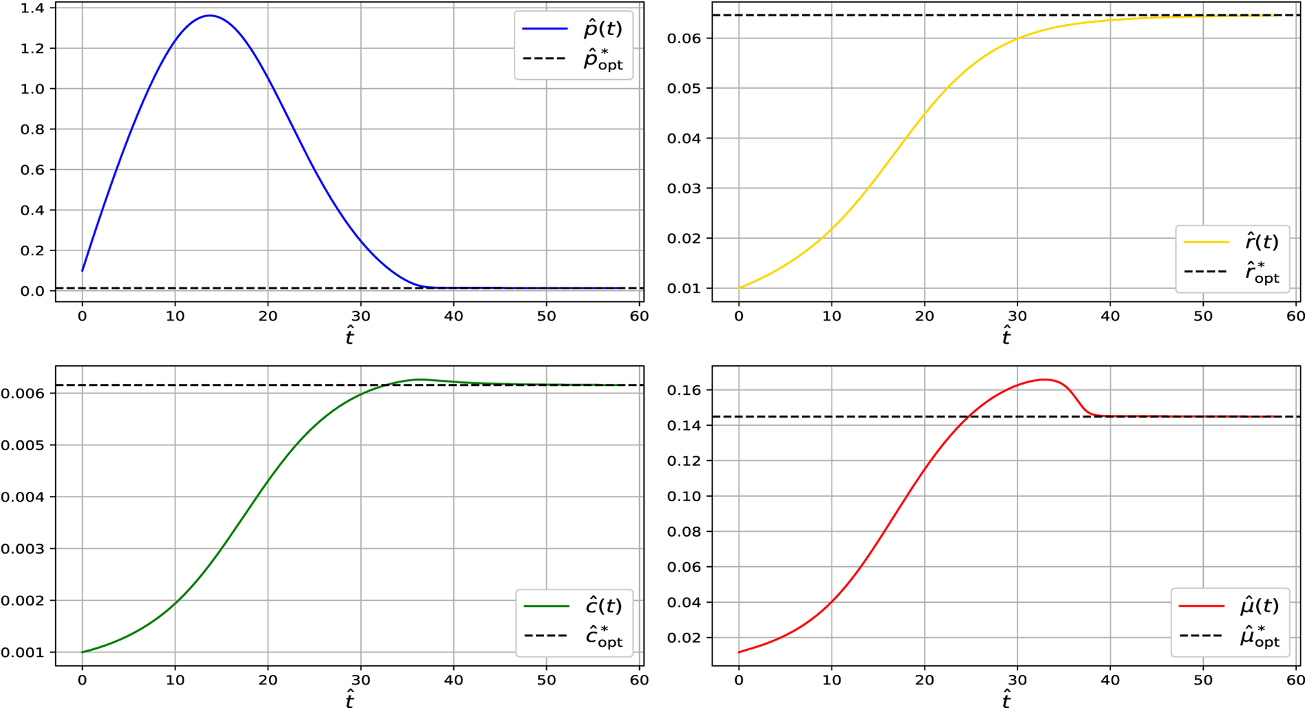
Figure 4: Simulation of the dynamical system showing convergence of
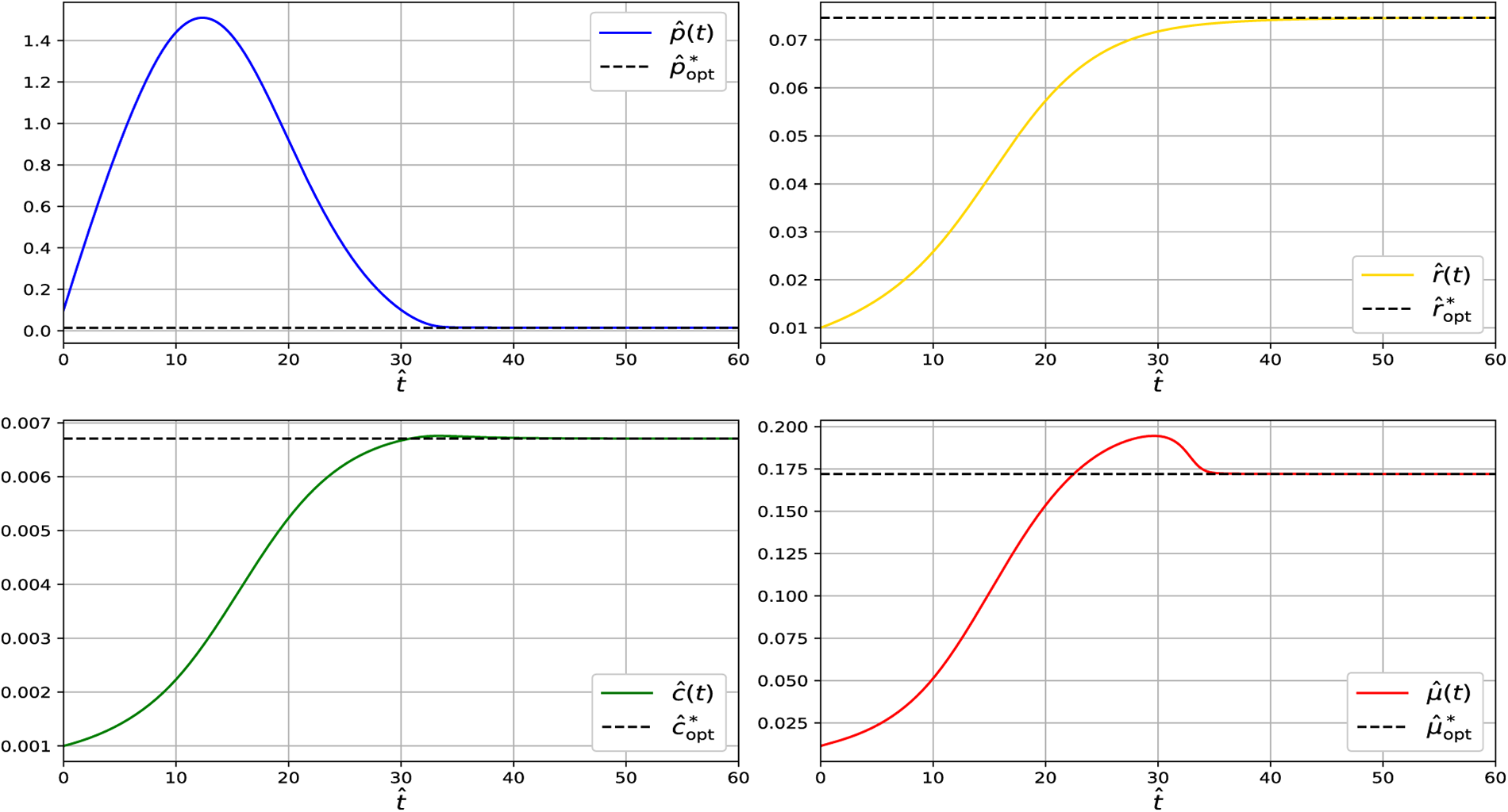
Figure 5: Simulation of the dynamical system showing convergence of
At steady state across the analyzed temperature range (13°C–19°C), the model predicts relatively small CspA fractions. This is consistent with growth-optimized proteome allocation, in which CspA acts primarily as a regulatory component rather than a dominant protein species. While CspA can reach high abundance during acute cold shock, such levels reflect transient stress responses following rapid temperature downshift and are not representative of adapted steady-state growth. Under steady conditions, excessive CspA expression imposes translational and metabolic costs, leading cells to preferentially allocate resources toward ribosomal and metabolic proteins, resulting in a minimal-sufficient CspA level.
The local stability of a steady state of a dynamical system can be assessed using the Jacobian matrix approach [22].
Theorem 1: A steady state is locally asymptotically stable if all the eigenvalues of the Jacobian matrix evaluated at the steady state have negative real parts.
For system (8), the Jacobian matrix J is obtained by differentiating the right-hand side with respect to the state variables
The Jacobian is evaluated at the steady state
Because of the strong nonlinearities, we compute the eigenvalues of the Jacobian matrix J numerically at each temperature’s steady state. The results are reported in Table 3.
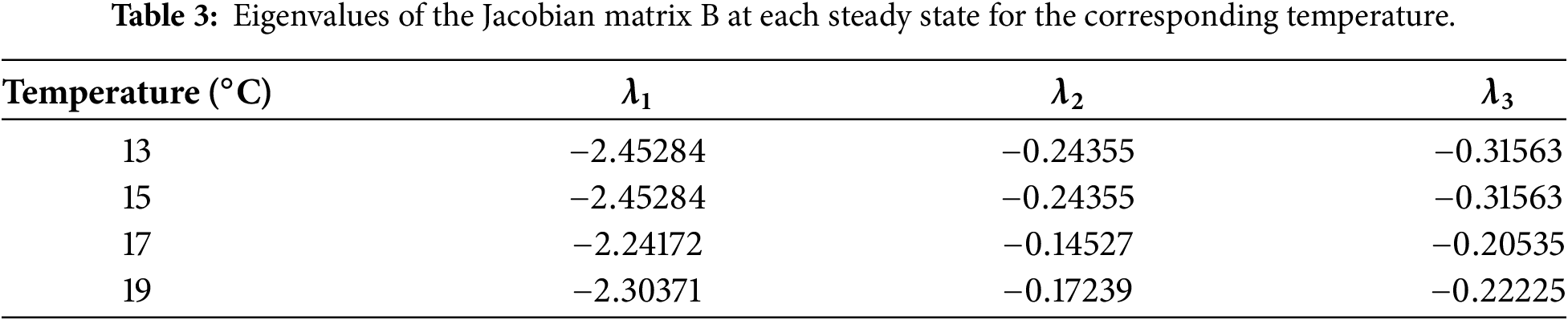
Across all temperatures examined (13°C–19°C), the Jacobian eigenvalues remain strictly negative, confirming that the steady state at each temperature is locally asymptotically stable. Together with the dynamical simulations (Figs. 2–5), which show that trajectories consistently converge to these steady states, the results demonstrate that the system reliably settles into its temperature-dependent equilibrium. This indicates that the qualitative stability properties of the model are preserved throughout the entire physiological temperature range analyzed.
We consider E. coli growth processes in the temperature range

Figure 6: Temperature-dependent behavior of the optimal dimensionless steady-state growth rate
Next, we analyzed how bacterial growth depends on the allocation parameter
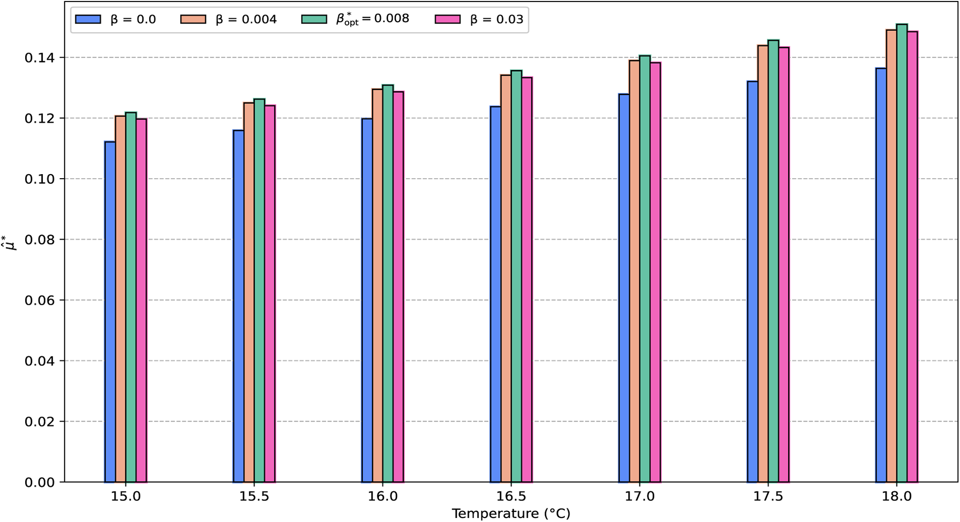
Figure 7: Effect of the control parameter
Optimal control theory provides a principled framework for quantifying how cells should allocate limited resources over time to maximize growth under environmental constraints [13,23–25]. In our setting, the control variables
where
which represents the cumulative biomass production over the time horizon
We assume that environmental variations, such as nutrient upshifts or downshifts, occur as instantaneous shifts [13]. For example, Escherichia coli transitions rapidly between habitats such as the mammalian gut, water bodies, soils, and sediments, where intermediate fluctuations are negligible. Each shift specifies a new value of the environmental input
Earlier studies formulated growth maximization as an infinite-horizon problem under the overtaking optimality criterion, implicitly assuming that trajectories reach and remain at the steady state corresponding to maximum growth rate. However, the formal existence of such overtaking optimal strategies was not proven, and infinite-horizon problems cannot be solved numerically. Finite-horizon simulations with free terminal states revealed small deviations from steady state near the end of the interval, regarded as artifacts under turnpike theory [26].
Following the approach of Yegorov et al. (2018) [13], we therefore consider two finite-horizon formulations: (i) without a terminal condition, where the final state is free, and (ii) with a fixed terminal condition, constraining the state variables to reach the steady state corresponding to maximum growth:
In optimal control theory, Pontryagin’s Maximum Principle (PMP) [27,28] provides the first-order necessary conditions for open-loop control strategies. The PMP has been used extensively in microbial resource-allocation models [9,13,22] and is well suited for the present problem, where the controls
where
which yields the following adjoint equations:
where
The Hamiltonian maximum conditions are
where the optimal controls
which is a necessary condition for an optimal open-loop control. An admissible process
that satisfies PMP conditions is called extremal. It is called normal if
If a switching function
Theorem 2 ([23]): Any singular arc
Proof: Assume that the process
where
On the singular arc for
as a convenient shorthand for the product term appearing in the switching functions. To compute the derivatives of the switching functions, we use the Poisson bracket operator
where
The first derivatives are
where
Along the singular arc, the first derivatives vanish identically, implying that
Now consider
which vanishes identically along the singular arc. To compute higher-order derivatives of
Applying this, we find
since
To ensure the singular arc is at least of order two, we must show
where
Substituting this expression into the previous equation yields
which equals zero along the switching surface since every term contains either
Numerical simulations of the optimal control problem were performed using the CasADi library in Python, employing the IPOPT solver with a relative tolerance of
For the free-final-state formulation (without terminal constraints), numerical simulations show that all state variables converge to their steady-state values
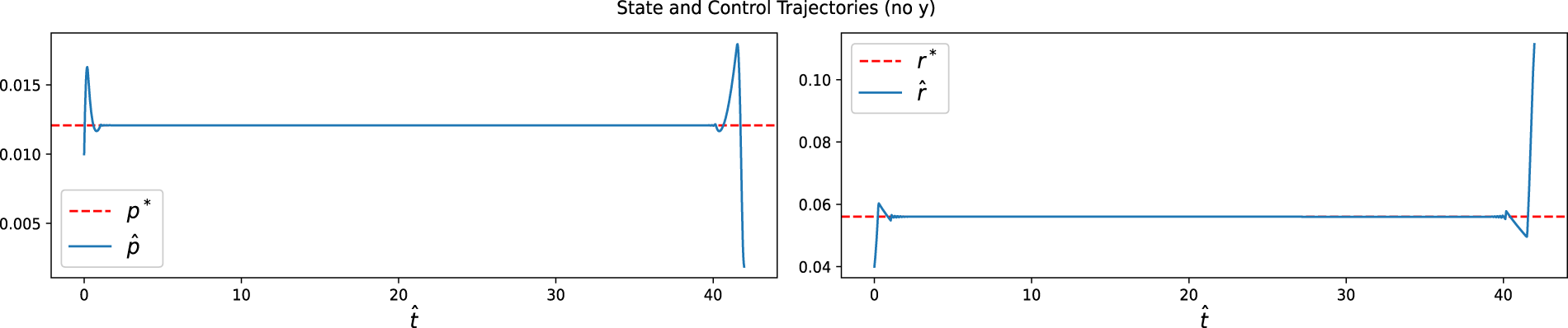
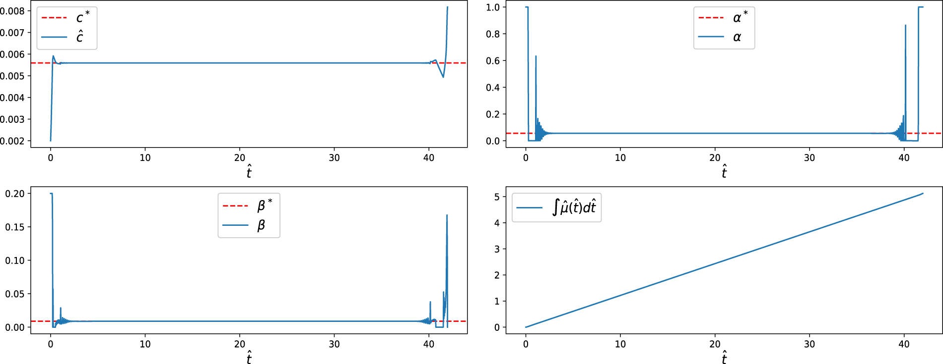
Figure 8: State and control trajectories for without a terminal condition. The dotted lines represent the steady-state optimal values, while the solid lines show the optimal trajectories. Both controls,
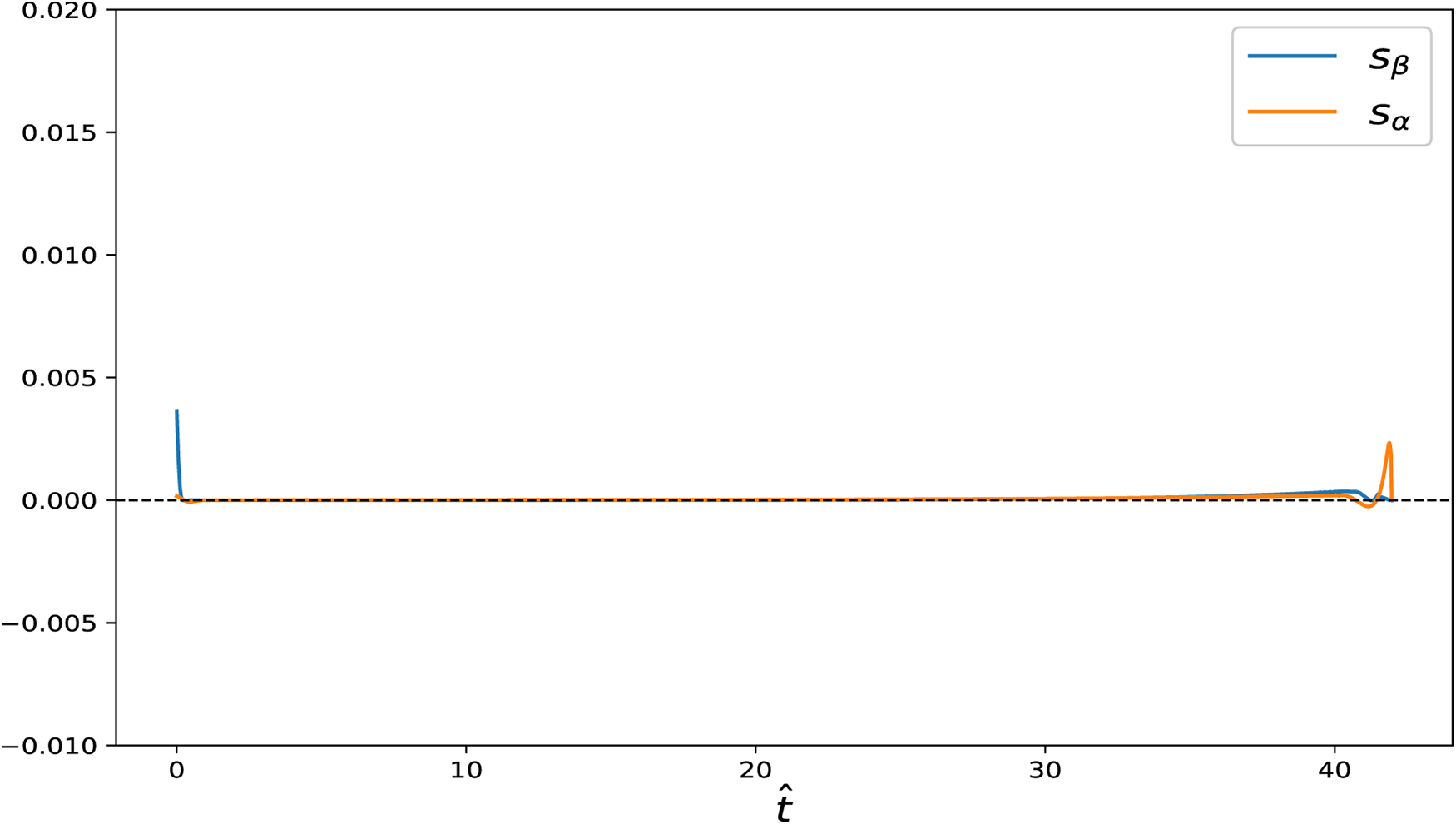
Figure 9: Switching functions
We further examined two specific cases in the free-final-state setting: (i)
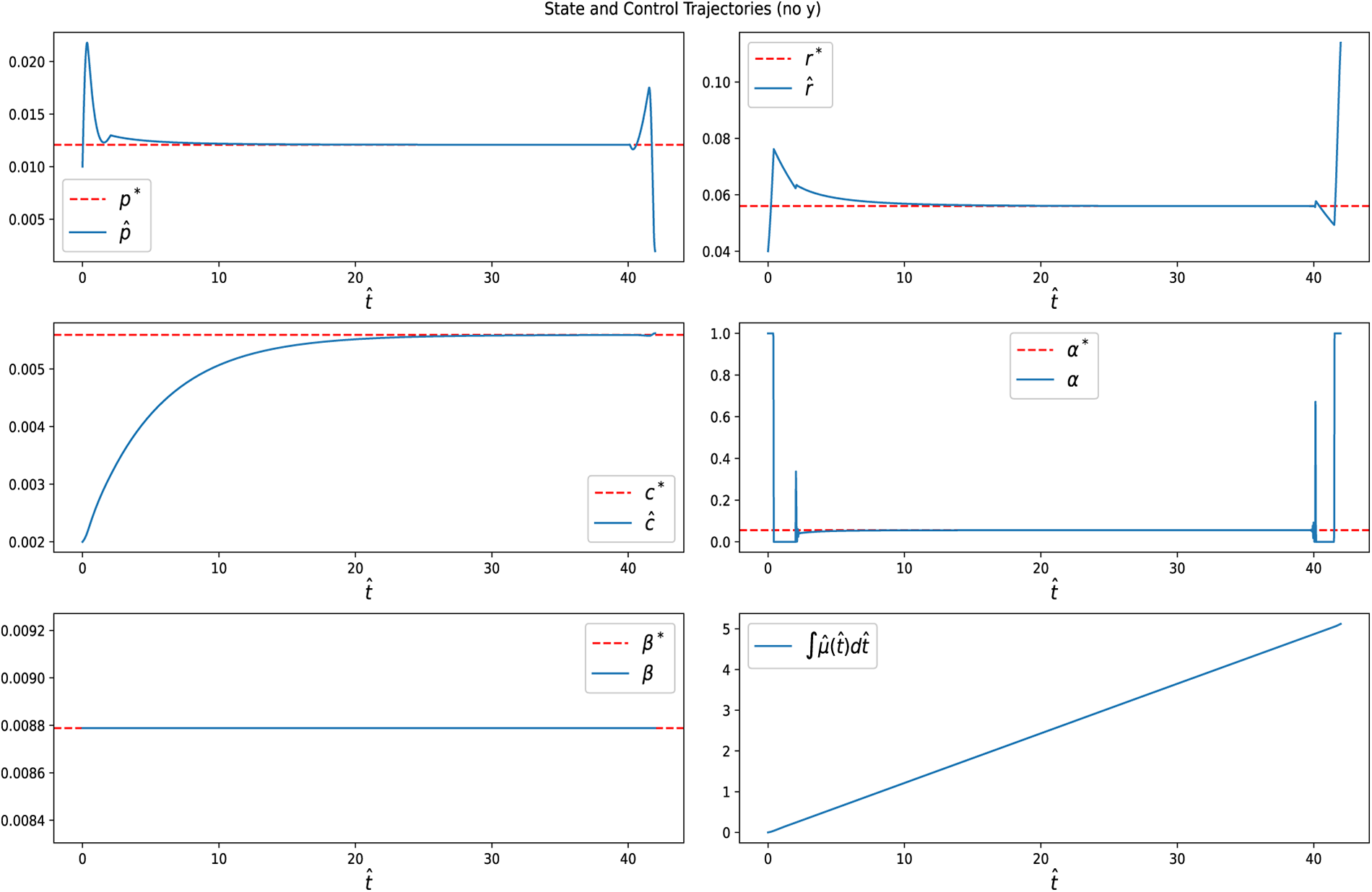
Figure 10: State variables and control input
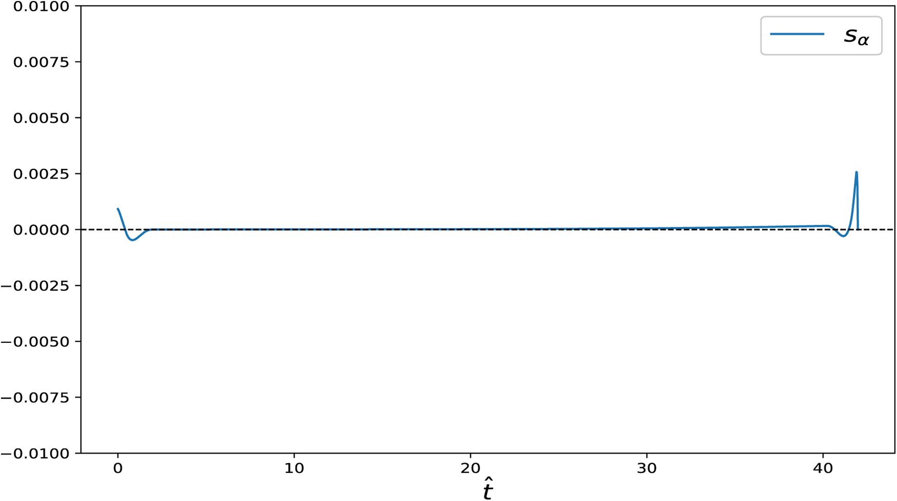
Figure 11: Switching function
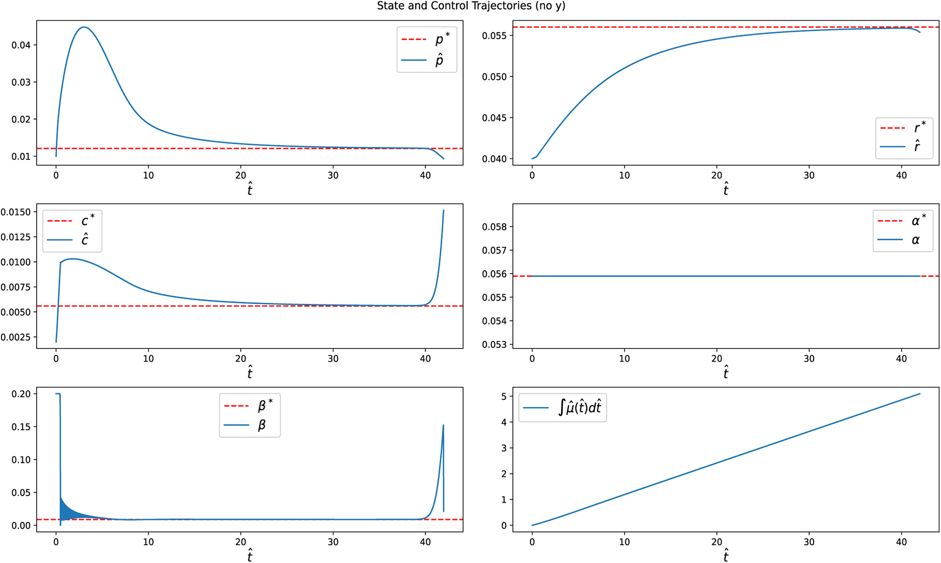
Figure 12: State variables and control input
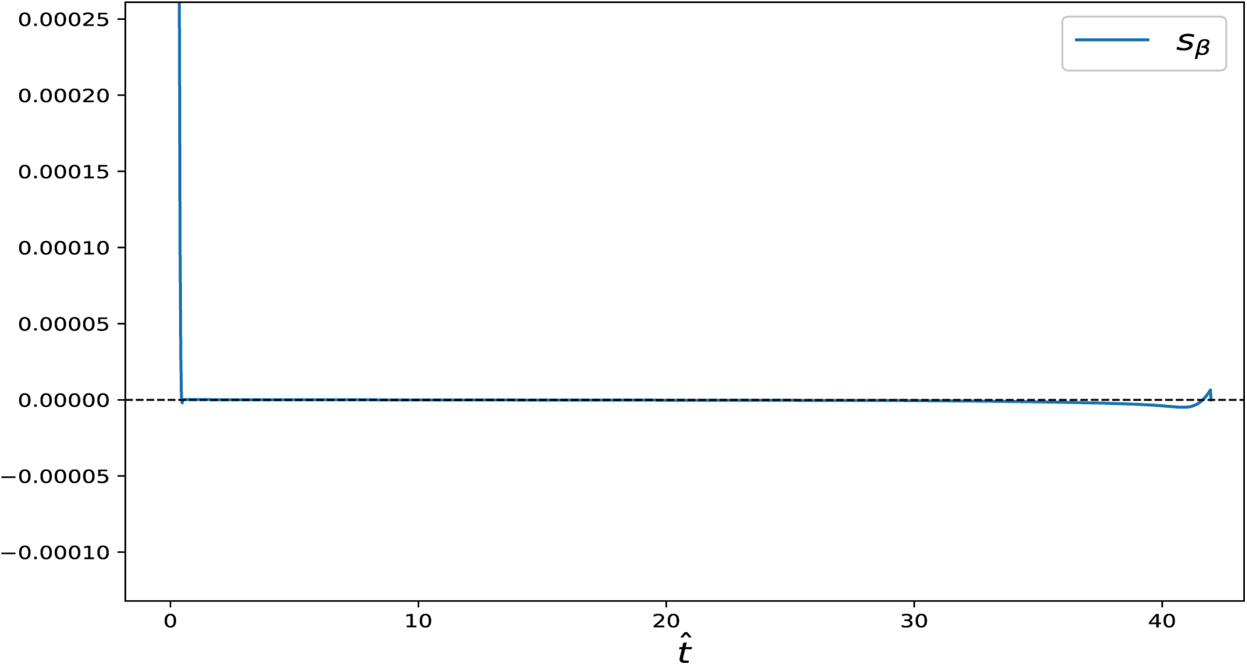
Figure 13: Switching function
When a terminal condition (11) is imposed, the system is required to reach the steady-state optimal allocation at the final time. Under this condition, both the state variables and controls remain at their steady-state values throughout the singular phase, effectively eliminating the final chattering arcs observed without the terminal condition (Fig. 14). Similar to the free-final-state case, we also examined scenarios with (i)
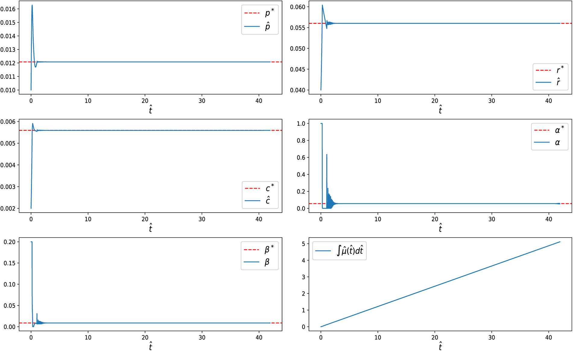
Figure 14: State variables and control inputs
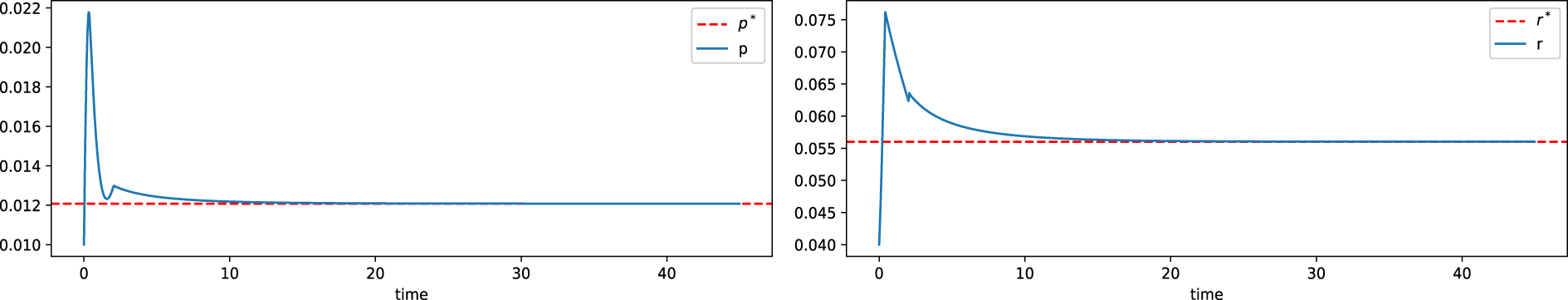
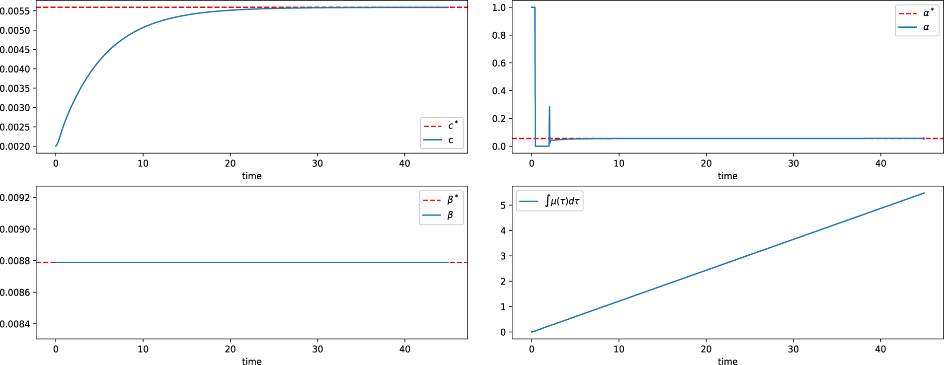
Figure 15: State variable and control input
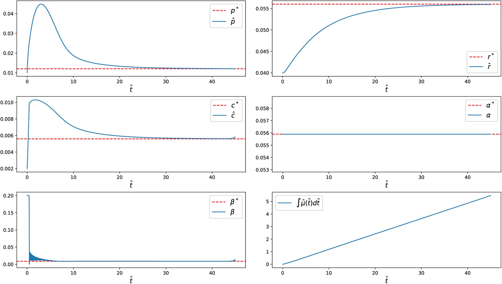
Figure 16: State variable and control input
Overall, the numerical results obtained using CasADi and IPOPT are fully consistent with the predictions of Pontryagin’s Maximum Principle. From a biological perspective, this behavior reflects rapid reallocation of translational resources during initial adjustment, followed by maintenance of a balanced growth state. The singular phase corresponds to sustained optimal proteome allocation, linking the bang-bang-singular control structure to bacterial adaptation under cold conditions.
In this study, we developed and analyzed a quantitative framework to investigate how Escherichia coli allocates limited cellular resources under cold-shock conditions, with particular emphasis on the role of the major cold-shock protein CspA. At low temperatures, the stabilization of mRNA secondary structures inhibits translation, reducing growth. CspA acts as an RNA chaperone that alleviates these inhibitory structures, thereby partially restoring translational efficiency. However, synthesizing CspA consumes translational capacity, creating a fundamental trade-off between stress response investment and biomass production. Incorporating CspA explicitly as a competing resource demand allowed us to capture the fundamental trade-off between stress-response investment and biomass production in a coarse-grained self-replicator model.
Across the temperature range considered (13°C–19°C), steady-state analysis revealed a distinct, locally stable equilibrium allocation of precursors, ribosomes, and CspA for each temperature. The predicted optimal investment in CspA remains small but nonzero, consistent with its role as a facilitator of translation rather than a major proteomic burden. Numerical simulations confirmed that system trajectories converge robustly to the temperature-specific steady states from initial conditions, indicating that the qualitative stability structure is preserved across physiologically relevant temperatures.
At the reference temperature (15°C), we examined the structure of optimal allocation using Pontryagin’s Maximum Principle. Our analysis revealed that the optimal allocation of resources exhibits a bang-bang-singular structure, where investment sharply shifts between biomass production and translational maintenance. This reflects the biological reality that bacteria must dynamically reallocate resources to respond efficiently to environmental changes, such as sudden temperature downshifts. While the exact bang-bang-singular pattern may not be fully realized in nature, it serves as a gold standard, providing a benchmark for understanding cellular decision-making and guiding the evaluation of real bacterial strategies.
Overall, this framework offers quantitative insight into how bacteria balance translational maintenance and biomass production during cold stress. By linking molecular aspects of the cold-shock response with optimal control theory, the study provides a foundation for interpreting bacterial adaptation strategies and suggests potential applications in synthetic biology and biotechnology, where improved performance at low temperatures is often desirable. Future work may include experimental validation, extension to multi-stress scenarios, the incorporation of additional biological constraints, and the development of adaptive or feedback-based strategies for quasi-optimal resource allocation. However, there are some limitations to this study: the model was developed for a restricted temperature range of
Acknowledgement: We would like to thank NASA Oklahoma Established Program to Stimulate Competitive Research (EPSCoR) Infrastructure Development, “Machine Learning Ocean World Biosignature Detection from Mass Spec” (PI: Brett McKinney), and Tandy School of Computer Science, University of Tulsa.
Funding Statement: This work was partly supported by NASA Oklahoma Established Program to Stimulate Competitive Research (EPSCoR) Infrastructure Development, “Machine Learning Ocean World Biosignature Detection from Mass Spec,” (PI: Brett McKinney), Grant No. 80NSSC24M0109, and Tandy School of Computer Science, The University of Tulsa.
Author Contributions: The authors confirm contribution to the paper as follows: Saira Batool: Conceptualization, Data curation, Formal analysis, Software, Validation, Writing—original draft. Muhammad Imran: Data curation, Formal analysis, Investigation, Project administration, Resources, Writing—review & editing. Brett McKinney: Supervision, Software, Validation, Visualization, Writing—review & editing. All authors reviewed and approved the final version of the manuscript.
Availability of Data and Materials: All data supporting the findings of this study are available in the article.
Ethics Approval: Not applicable.
Conflicts of Interest: The authors declare no conflicts of interest.
References
1. Barria C, Malecki M, Arraiano CM. Bacterial adaptation to cold. Microbiology. 2013;159(Pt_12):2437–43. doi:10.1099/mic.0.052209-0. [Google Scholar] [PubMed] [CrossRef]
2. Zhang Q, Li R, Li J, Shi H. Optimal allocation of bacterial protein resources under nonlethal protein maturation stress. Biophys J. 2018;115(5):896–910. doi:10.1016/j.bpj.2018.07.021. [Google Scholar] [PubMed] [CrossRef]
3. Ehrenberg M, Bremer H, Dennis PP. Medium-dependent control of the bacterial growth rate. Biochimie. 2013;95(4):643–58. doi:10.1016/j.biochi.2012.11.012. [Google Scholar] [PubMed] [CrossRef]
4. Serbanescu D, Ojkic N, Banerjee S. Cellular resource allocation strategies for cell size and shape control in bacteria. FEBS J. 2022;289(24):7891–906. doi:10.1111/febs.16234. [Google Scholar] [PubMed] [CrossRef]
5. Trickovic B, Lynch M. Resource allocation to cell envelopes and the scaling of bacterial growth rate. Phys Biol. 2025;22(4):046002. doi:10.1101/2022.01.07.475415. [Google Scholar] [CrossRef]
6. Dourado H, Lercher MJ. An analytical theory of balanced cellular growth. Nat Commun. 2020;11(1):1226. doi:10.1101/607374. [Google Scholar] [CrossRef]
7. Scott M, Gunderson CW, Mateescu EM, Zhang Z, Hwa T. Interdependence of cell growth and gene expression: origins and consequences. Science. 2010;330(6007):1099–102. doi:10.1126/science.1192588. [Google Scholar] [PubMed] [CrossRef]
8. Jiang W, Hou Y, Inouye M. CspA, the major cold-shock protein of Escherichia coli, is an RNA chaperone. J Biol Chem. 1997;272(1):196–202. doi:10.1074/jbc.272.1.196. [Google Scholar] [PubMed] [CrossRef]
9. Giuliodori AM, Belardinelli R, Duval M, Garofalo R, Schenckbecher E, Hauryliuk V, et al. Escherichia coli CspA stimulates translation in the cold of its own mRNA by promoting ribosome progression. Front Microbiol. 2023;14:1118329. doi:10.3389/fmicb.2023.1118329. [Google Scholar] [CrossRef]
10. Ivancic T, Jamnik P, Stopar D. Cold shock CspA and CspB protein production during periodic temperature cycling in Escherichia coli. BMC Res Notes. 2013;6(1):248. doi:10.1186/1756-0500-6-248. [Google Scholar] [CrossRef]
11. Li H, Giuliodori AM, Wang X, Tian S, Su Z, Gualerzi CO, et al. Cold shock proteins mediate transcription of ribosomal RNA in Escherichia coli under cold-stress conditions. Biomolecules. 2025;15(10):1387. doi:10.3390/biom15101387. [Google Scholar] [PubMed] [CrossRef]
12. Giuliodori AM, Di Pietro F, Marzi S, Masquida B, Wagner R, Romby P, et al. The cspA mRNA is a thermosensor that modulates translation of the cold-shock protein CspA. Mol Cell. 2010;37(1):21–33. doi:10.1016/j.molcel.2009.11.033. [Google Scholar] [PubMed] [CrossRef]
13. Yegorov I, Mairet F, Gouzé JL. Optimal feedback strategies for bacterial growth with degradation, recycling, and effect of temperature. Optim Control Appl Methods. 2018;39(2):1084–109. doi:10.1002/oca.2398. [Google Scholar] [CrossRef]
14. Imizcoz JI, Djema W, Mairet F, Gouzé JL. Optimal control of a microbial growth model by means of substrate concentration and resource allocation. IFAC-PapersOnLine. 2025;59(6):528–33. doi:10.1016/j.ifacol.2025.07.200. [Google Scholar] [CrossRef]
15. Weiße AY, Oyarzún DA, Danos V, Swain PS. Mechanistic links between cellular trade-offs, gene expression, and growth. Proc Natl Acad Sci U S A. 2015;112(9):E1038–47. doi:10.1073/pnas.1416533112. [Google Scholar] [PubMed] [CrossRef]
16. Molenaar D, Van Berlo R, De Ridder D, Teusink B. Shifts in growth strategies reflect tradeoffs in cellular economics. Mol Syst Biol. 2009;5(1):323. doi:10.1038/msb.2009.82. [Google Scholar] [PubMed] [CrossRef]
17. Yabo AG. Optimal control strategies in a generic class of bacterial growth models with multiple substrates. Automatica. 2025;171(5):111881. doi:10.1016/j.automatica.2024.111881. [Google Scholar] [CrossRef]
18. Mairet F, Gouzé JL, De Jong H. Optimal proteome allocation and the temperature dependence of microbial growth laws. npj Syst Biol Appl. 2021;7(1):14. doi:10.1038/s41540-021-00172-y. [Google Scholar] [PubMed] [CrossRef]
19. Martinez G, Pachepsky YA, Shelton DR, Whelan G, Zepp R, Molina M, et al. Using the Q10 model to simulate E. coli survival in cowpats on grazing lands. Environ Int. 2013;54:1–10. doi:10.1016/j.envint.2012.12.013. [Google Scholar] [PubMed] [CrossRef]
20. Storn R, Price K. Differential evolution—a simple and efficient heuristic for global optimization over continuous spaces. J Glob Optim. 1997;11(4):341–59. doi:10.1023/a:1008202821328. [Google Scholar] [CrossRef]
21. Fiedler A, Raeth S, Theis FJ, Hausser A, Hasenauer J. Tailored parameter optimization methods for ordinary differential equation models with steady-state constraints. BMC Syst Biol. 2016;10(1):80. doi:10.1186/s12918-016-0319-7. [Google Scholar] [PubMed] [CrossRef]
22. Strogatz SH. Nonlinear dynamics and chaos: with applications to physics, biology, chemistry, and engineering. Boca Raton, FL, USA: Chapman and Hall/CRC; 2024. [Google Scholar]
23. Yabo AG, Caillau JB, Gouzé JL. Optimal bacterial resource allocation: metabolite production in continuous bioreactors. Math Biosci Eng. 2020;17(6):7074–100. [Google Scholar] [PubMed]
24. Augier N, Yabo AG. Time-optimal control of piecewise affine bistable gene-regulatory networks. Int J Robust Nonlinear Control. 2023;33(9):4967–88. doi:10.1002/rnc.6012. [Google Scholar] [CrossRef]
25. Yabo AG, Caillau JB, Gouzé JL. Optimal bacterial resource allocation strategies in batch processing. SIAM J Appl Math. 2024;84(3):S567–91. doi:10.1137/22m1506328. [Google Scholar] [CrossRef]
26. Trélat E, Zuazua E. The turnpike property in finite-dimensional nonlinear optimal control. J Differ Equ. 2015;258(1):81–114. doi:10.1016/j.jde.2014.09.005. [Google Scholar] [CrossRef]
27. Lenhart S, Workman JT. Optimal control applied to biological models. Boca Raton, FL, USA: Chapman and Hall/CRC; 2007. [Google Scholar]
28. Pontryagin LS. Mathematical theory of optimal processes. London, UK: Routledge; 2018. [Google Scholar]
29. Van der Schaft AJ. Symmetries in optimal control. SIAM J Control Optim. 1987;25(2):245–59. doi:10.1137/0325015. [Google Scholar] [CrossRef]
Cite This Article
 Copyright © 2026 The Author(s). Published by Tech Science Press.
This work is licensed under a Creative Commons Attribution 4.0 International License , which permits unrestricted use, distribution, and reproduction in any medium, provided the original work is properly cited.
 Downloads
 Citation Tools