A Unified Deep Supervised Network for Effective Animal Voice Recognition

1  Introduction

In recent decades, animal species identification/recognition has been an extremely important area of research and has extensive applications in domains such as wildlife conservation, animal behavior analysis, habitat monitoring, and ecological research. It provides an organized context for grouping and recognizing the massively diverse range of animal species on Earth [1–3]. Therefore, approximately 2.17 million species have been formally described worldwide, while the total number of species on Earth remains uncertain because many species have yet to be discovered and described. Animals represent one of the major groups of global biodiversity, including mammals, birds, amphibians, fish, reptiles, and invertebrates [4]. There are approximately 6815 species of mammals, with a remarkable variety of adaptations that allow them to thrive in various habitats, which can be classified into two groups, namely domestic animals and wildlife. Examples of the former include cats, dogs, cows, sheep, etc., whereas wildlife animals are bears, lions, monkeys, and rhinoceroses, among others. Both domestic and wildlife animals play crucial roles in biodiversity, agriculture and food production, textiles and materials, search and rescue, and particularly human-animal relationships [5,6]. The ability to identify these animals can significantly aid in preservation efforts, protection from hazards, and the promotion of biodiversity, sustainable agriculture, and effective ecosystem management, and is made possible via different forms of sensor data. In recent years, biodiversity has begun to decrease rapidly worldwide, necessitating the immediate and cost-effective deployment of scalable monitoring systems to better study and understand the behavior of domestic and wild animals. These scalable monitoring systems rely on vision and acoustic sensors to capture diverse data across diverse environments [7]. The vision and acoustic sensors are considered the primary sources of data that can help in monitoring bioacoustics, wildlife management, a greater understanding of conservation, understanding of human-animal interactions, and species identification/recognition [8]. These sensors generate a huge amount of raw data, and processing, monitoring, and analysis of this data can be both labor-intensive and time-consuming [9]. To cope with this, researchers proposed several artificial intelligence-based methods to effectively recognize various animal species [10]. For instance, Clemins et al. [11], presented a hidden Markov model for African elephant breed recognition. Hu et al. [12], developed a hybrid wireless acoustic sensor network to carry out a census of the populations of cane toads and native frogs in Australia. A method based on the mel-frequency cepstral coefficient (MFCC) and Gaussian mixture model was proposed by Cheng et al. [13] to recognize the voices of different birds. Yeo et al. [14] proposed an approach that combined the zero-crossing rate, MFCC, and dynamic time warping (DTW) for animal voice recognition. The zero-crossing rate was used to detect the endpoint of the input voice, in order to remove silence, whereas the MFCC was applied to obtain compact and non-redundant features, and the DTW was used for pattern classification. In another study, Mel cepstral coefficient features were extracted from the vocalizations of pigs, and recognition was carried out with a sparse representation classifier [15]. Salamon et al. [16] utilized convolutional neural network (CNN) methods for the classification of insect and bird sounds. MFCC features were initially extracted from raw data, and a CNN architecture was then used for further refinement and classification. In [17], a system was developed to recognize the voices of anurans using a CNN and a support vector machine (SVM), where the CNN was used for audio feature extraction and the SVM for final classification. The researchers in [18] employed an MFCC feature extraction mechanism to select the optimal features from the given input voice and fed them to a CNN architecture for further refinement and classification. These authors also developed a new animal voice dataset based on the sounds of 10 species collected from online sources, and their model achieved an accuracy of 75%. Kyungdeuk et al. [19] proposed a new channel and frequency attention module with a pre-trained CNN model for the classification of diverse animal sounds. Bishop et al. [6] proposed an effective model based on MFCC, discrete wavelet transform (DWT), and SVM to effectively classify farm soundscapes for livestock vocalization. In [20], the researcher developed a CNN-based method for animal voice recognition (AVR) in a noisy environment using two streams. Nanni et al. [21] developed an ensemble classifier for automatic bird and cat voice recognition and conducted experiments with five different CNN architectures on both original and augmented datasets to improve performance. Nanni et al. [22] combined Siamese neural networks with different clustering approaches to enable the determination of the center points of the spectrum, the processing of spectral features, the calculation of the similarity space, and the exploitation of dissimilarity vectors for classification. Xu et al. [23] presented a multi-view CNN model consisting of three convolution layers with three different filter lengths in parallel, in order to extract long-, medium-, and short-term information at the same time. They performed experiments on two benchmarks, and their scheme achieved promising performance.

Furthermore, ref. [27] proposed a threshold-based approach that incorporated the features of short-time energy, Wiener entropy, and cepstral peak prominence for monitoring the health status of poultry. This is considered an essential subject for various reasons, including the importance of chickens as a significant source of food for humans and the prevalence of disease outbreaks. For use in poultry farming, ref. [5] proposed three different network models, called PV-net1, PV-net2, and PV-net3, to classify the normal and eating-related vocalizations of poultry, based on recordings of 18 different chickens. Ref. [24] were able to recognize five different bird species by extracting the MFCC features from audio data and applying a multi-layer perceptron (MLP) classifier. A one-dimensional local binary pattern and a tunable Q wavelet transform for feature extraction in both the frequency and space domains for the recognition of anuran voices is proposed in [28]. They also created a new dataset of anuran sounds comprising 1536 voice recordings from 26 anuran species. In another approach [29], a convolutional recurrent neural network-based model was used to automatically detect the calls of chimpanzees. They also used several strategies to address class imbalance, including spectrogram denoising, alternative loss functions, and resampling. By applying these strategies, they improved their model’s performance compared to other state-of-the-art methods. Kim et al. [9], proposed an approach based on vision and acoustic sensors for the recognition of 15 different animal species using deep learning. They proposed two multimodality datasets containing visual and audio data for the AVR. They also trained two different deep learning models to analyze visual and audio data, with visual features extracted using EfficientNetB0 and audio features using MFCCs. Finally, a modified Visual Geometry Group (VGG) was used for classification. Next [25] proposed a light-CNN model called VGG11 to automatically recognize distress in chickens from 1973 recordings of normal vocalizations and 3363 distress calls. They used data augmentation approaches to increase the amount of training data, and their scheme achieved an average accuracy of 95.07%. Shorten & Hunter [26] developed a collar that included acoustic sensors to differentiate between vocalizations by cows and background sounds. They used a CNN model to classify cow vocalizations into three classes (open, closed, and mixed mouth noises) and applied a bidirectional long short-term memory network (BiLSTM) to estimate the duration of each vocalization. Tao et al. [30] proposed a feature extraction process based on linear and nonlinear fusion with a random forest classifier for the health monitoring of white-feather broilers. In [31], the authors combined four different approaches for signal filtering, classification, machine learning, and sparse representation to propose a filtering and classification model for white-feather broiler sounds based on sparse representation.

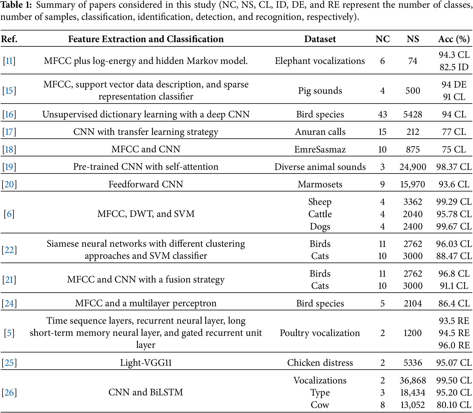
Existing approaches in this area have several limitations; for example, they typically involve extracting features and passing them to machine learning classifiers such as MLPs or SVMs, while recent approaches mainly employ deep learning architectures for AVR, as shown in Table 1. These features include statistical measures (e.g., median, mean, variance), MFCC, fast Fourier transform (FFT) spectra, wavelets, spectrograms, and Wigner-Ville distributions (WVDs). Traditional feature extraction and classification approaches require extensive calibration, and the classifiers rely heavily on the quality of the extracted features, meaning that domain knowledge and engineering expertise are required for robust feature extraction. In addition, traditional feature extraction is time-consuming and resource-intensive. To cope with these challenges, deep learning-based methods have been increasingly used for their ability to automatically extract salient features. However, these methods also have limitations, such as the need for further refinement and selection of extracted features, high computational hardware requirements, and large amounts of training data. Furthermore, existing methods in the animal voice recognition domain often face data limitations. Mostly, the available datasets consist of a limited number of classes or an insufficient number of samples. Additionally, many of the datasets used in the previous studies are not publicly available, further hindering progress in this field. These approaches, therefore, lack the scalability demanded by new applications.

1.1 Research Objectives

The main objective of the proposed work is to advance the AVR field by addressing key challenges related to species recognition from vocalizations. In this research work, the main focus is to develop an efficient method for representing voice signals by transforming them into two-dimensional (2D) spectrograms, which is significant for effective voice classification. The proposed work also introduces an efficient CNN model, AVRNet, that incorporates depthwise-separable convolutions and a modified attention mechanism for focused recognition of animal species. Our study includes the creation of a comprehensive animal species recognition dataset, with a view to overcoming the limitations of existing datasets, which represents a valuable asset for research into wildlife care systems and conservation. Through an empirical validation process, a comparison of AVRNet with state-of-the-art approaches, and an ablation study, demonstrate the efficiency and effectiveness of our proposed model in terms of advancing AVR research. The major contributions of this research work are as follows:

•   2D voice signal representation with spectrograms: In the proposed research, voice signals are transformed into a 2D representation through spectrograms, which can be used as visual representations of voice signals. The spectrograms show the signal intensity across various frequencies over time. The short-term Fourier transform (STFT) is used to obtain this representation, allowing the FFT to process the Fourier spectrum for each signal segment. This transformation into spectrogram representations is crucial for developing an effective voice classification and recognition system, as it facilitates the extraction of rich, salient features.

•   Efficient CNN model with multi-scale feature extraction: The proposed work introduces an efficient CNN model that employs depthwise-separable convolutions, which reduces the number of learning parameters and computational complexity. Multi-scale feature extraction improves the performance for objects of varying sizes (varying voice durations in the spectrograms), enhances robustness to variations in the spectrograms, and effectively captures diverse acoustic patterns. A modified attention mechanism is also integrated with the proposed model to focus on more critical features for effective animal species recognition.

•   Animal species recognition dataset: In this research work, a new medium-scale dataset is created for animal species recognition with the aim of addressing the limitations of existing datasets, which often focus on specific species and have only small numbers of instances for training. The proposed dataset comprises 15 animal species and accommodates imbalances in the number of audio clips per class. The proposed work also includes a “silent/noisy class” for silent clips or background noise monitoring, with the aim of supporting developments in wildlife care systems and conservation research.

•   Experimental validation: Comprehensive experiments are performed on two datasets, including a benchmark dataset and a proposed custom dataset, to provide empirical validation of the efficiency and effectiveness of our model. Through these experiments, the proposed model is compared with state-of-the-art approaches. Furthermore, an ablation study and statistical test of the proposed model using metrics such as accuracy, precision, recall, and F1-score confirm the robustness and reliability of the proposed model and demonstrate its value as a tool for AVR research.

1.2 Paper Organization

The rest of the paper is organized as follows. Section 2 provides an in-depth discussion of the preprocessing stages and the proposed model. Section 3 presents the evaluation metrics, datasets, and comparative analysis. Section 4 discusses the results and their implications. Finally, Section 5 concludes the paper and outlines directions for future research.

2  Proposed Framework

AVR has recently attracted significant attention from the research community, and deep learning-based methods have emerged as the leading approach in this domain due to their notable performance [16,19,25]. Therefore, an efficient and effective CNN-based architecture is developed for animal voice recognition. Our work includes a crucial additional step to transform voice signals into spectrograms, thus enabling a visual representation of the signal intensity across frequencies over time using the STFT technique. All components of our model, including the transformation of voice signals into image-like spectrograms and the details of the proposed CNN, are described in depth in the following sections.

2.1 Generation of Spectrograms

The conversion of a voice signal into a 2D representation plays a significant role in several research domains, as explained in [21,32]. A spectrogram represents a voice signal in 2D and provides a useful visualization of a voice recording, showing the intensity of the signal across various frequencies. For this purpose, the STFT is used, in which the signal is segmented into short, fixed-length frames and the FFT is applied to obtain the Fourier spectrum of each frame. The resulting spectrogram shows the frequency content over time, where the x-axis represents time (t) and the y-axis represents frequency (f), as shown in Fig. 1 and Eq. (1).

X(τ,ω)=∫−∞∞S(t)f(t−τ)e−iωtdt.(1)

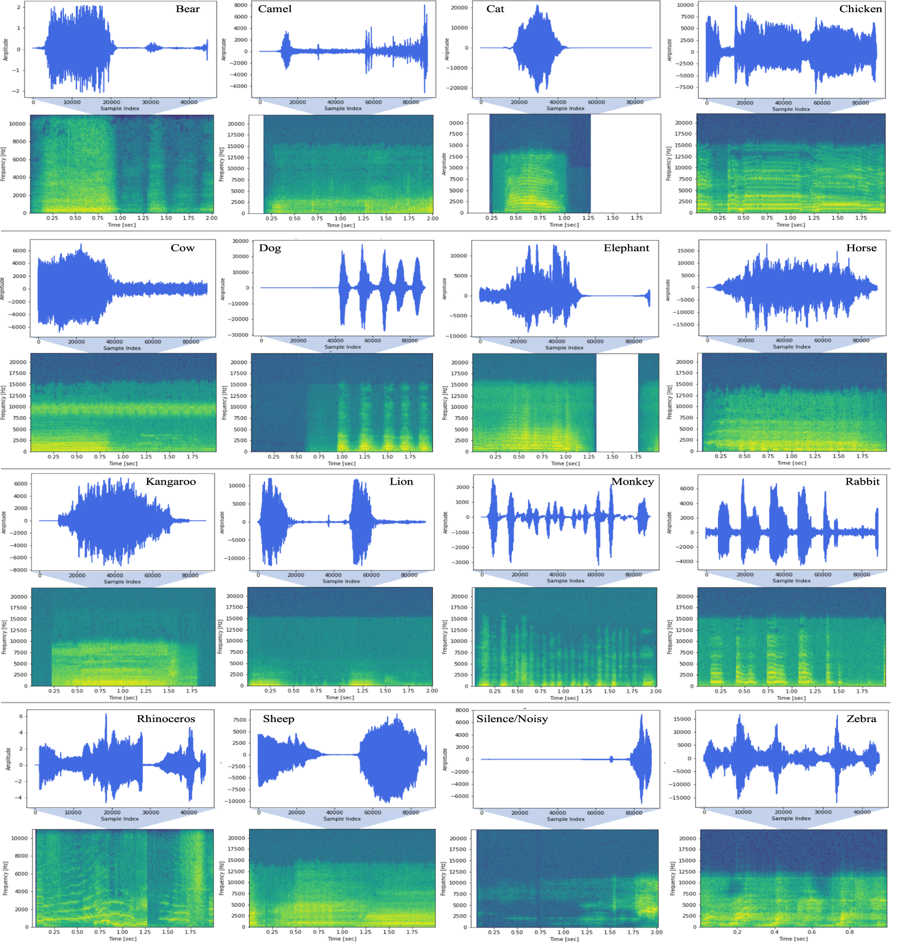
Figure 1: Conversion of the waveform into a spectrogram for effective AVR classification.

As indicated above, speech spectrogram S encompasses a range of frequencies distributed across various time intervals S (t, f) for each voice signal. In machine learning, the STFT is widely used for audio preprocessing because it produces a 2D representation that jointly captures time and frequency information. It is effective for localizing events, extracting salient features, and recognizing patterns in acoustic data, making it suitable for tasks such as music analysis, sound event detection, and speech recognition. Its ability to handle time variations while providing a clear frequency breakdown makes it a suitable choice for training deep learning models on audio datasets [33,34].

All recordings used in the proposed work were first resampled to a sampling rate of 22.05 kHz. The original recordings were collected from heterogeneous sources and had different native sampling rates. Specifically, the complete dataset comprised 3848 recordings originally sampled at 44.1 kHz, including recordings from local sources in Pakistan, YouTube, and silence/noise samples; 503 recordings originally sampled at 22.05 kHz, including recordings from EmreSasmaz, Facebook, and National Geographic; and 27 recordings from Facebook originally sampled at 48 kHz. Multi-channel recordings were converted to mono by retaining the first channel. The STFT was computed using a Tukey window (shape parameter α = 0.25) with a window length of 256 samples (≈11.6 ms), an FFT size of 256, and an overlap of 32 samples, corresponding to a hop length of 224 samples (≈10.2 ms). The transform returned the power spectral density (power scaling), to which a natural-logarithm compression was applied to reduce the dynamic range; no decibel (10·log10) conversion was used. The STFT parameters were selected to provide an effective compromise between temporal and spectral resolution for animal vocalizations. The selected FFT size and window length provide sufficient frequency resolution to capture harmonic structures and species-specific spectral characteristics, while the chosen hop length preserves adequate temporal continuity without introducing excessive redundancy. The Tukey window (α = 0.25) tapers only the outer 25% of each frame with a cosine profile while leaving the central region flat, providing a balance between the low spectral leakage of a fully tapered window and the resolution of a rectangular window. Each log-power spectrogram was normalized to the range [0, 1] using per-image min–max scaling and rendered with the perceptually uniform viridis colormap, in which higher log-power values appear brighter and lower values darker. Per-image min–max normalization scales each spectrogram to a common [0, 1] range but removes the absolute amplitude information of the original recording. As a result, recordings with similar spectral structures but different recording gains produce identical normalized spectrograms. This is an intentional trade-off because our dataset is compiled from heterogeneous sources, including local field recordings and publicly available online recordings, where recording gain, microphone characteristics, and environmental conditions introduce significant amplitude variability. Consequently, scale-invariant time–frequency patterns provide more reliable cues for species recognition than absolute loudness, and this normalization also improves numerical stability during training.

2.2 Proposed Model for AVR

To address the challenges in AVR, the proposed research leverages the adaptability of CNN models, which have traditionally excelled across a wide range of computer vision tasks, including object detection, segmentation, recognition, localization, identification, and classification. Their use in voice classification is inspired by the remarkable success of CNN models in related domains. The basic building blocks of a CNN model include convolutional layers, pooling layers, and dense layers. Convolutional layers are designed with a variety of filters to extract distinctive features from the input data, whereas pooling layers play a significant role in reducing the input dimensions, and dense layers combine the extracted features into a global representation used for classification. The extracted features are then passed to the output layer (SoftMax function), which outputs distinct probabilities for different classes. In the proposed research, a novel CNN architecture AVRNet is proposed, which is composed of several layers and components that are carefully designed to learn and extract meaningful features from the data input. The input of the AVRNet model has dimensions of 224 × 224 × 3, followed by several core blocks designed for deep feature extraction. An attention mechanism is incorporated to refine these features, and a SoftMax layer is used for the final classification, as shown in Fig. 2.

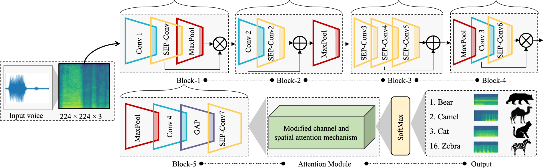
Figure 2: General framework of the proposed AVRNet for AVR.

In the proposed AVRNet model, the first block consists of three different types of layers, such as convolutional, separable convolutional, and max pooling. The convolutional layer employs 64 kernels of size 3 × 3 to extract low-level spatial and spectral features from the input spectrograms. Subsequently, a separable convolutional layer with 64 filters and a kernel size of 3 × 3 is utilized to reduce computational complexity and parameter overhead compared with standard convolution operations. A max-pooling layer with a pool size of 2 × 2 is then applied to reduce the spatial dimensions while preserving the most informative features. The second block consists of a standard convolutional layer with 128 filters of size 3 × 3, followed by a separable convolutional layer with 128 filters of the same size. The outputs of both layers are added using a feature fusion strategy to preserve complementary feature information extracted by conventional and separable convolutions. A max-pooling layer is then applied for dimensionality reduction. The third block of the proposed model has three separable convolution layers, each layer utilizes 256 filters with a size of 3 × 3. A skip connection is then used to add the output features from the second and third layers, followed by a max-pooling layer. Additionally, a multi-scale feature fusion strategy is adopted by combining features from different convolutional layers. The multiple convolution operations with 3 × 3 filters are used to extract rich and intricate features. This strategy allows the model to capture rich hierarchical representations and detailed spectrogram patterns while effectively learning discriminative features. Afterwards, a max-pooling operation is applied. In addition, an auxiliary classification branch is connected after Block 3 to implement hierarchical deep supervision during training. Each auxiliary branch consists of a Global Average Pooling layer followed by a dense layer containing 64 neurons, dropout regularization, and a SoftMax classifier. This auxiliary classifier helps strengthen gradient propagation to intermediate layers, improves feature discriminability, and accelerates network convergence.

The fourth block consists of a conventional convolutional layer with 256 filters, followed by a separable convolutional layer with 512 filters. The extracted feature maps are concatenated to preserve complementary local and global representations before being passed to a max-pooling layer. Similar to Block 3, another auxiliary classifier is connected after Block 4 to provide additional supervision during training. The auxiliary classifier structure is identical to that used in Block 3 and contributes to improving training stability and reducing vanishing gradient issues. These auxiliary classifiers are used only during the training stage and are removed during inference/testing.

The fifth block includes a conventional convolutional layer with 256 filters with 3 × 3 kernel and a separable convolutional layer with 512 filters and a 3 × 3 kernel. The outputs of these layers are concatenated and passed through a 2 × 2 max-pooling layer. The combination of standard and separable convolutions across multiple stages enables AVRNet to perform multi-scale feature extraction by learning both local fine-grained patterns and broader contextual representations from spectrogram inputs. After deep feature extraction, the proposed AVRNet incorporates a modified channel-spatial attention mechanism to refine discriminative feature representations. The detailed mathematical formulation and working mechanism of the proposed attention module are presented in Section 2.3. Following the attention mechanism, Global Average Pooling (GAP), fully connected layers, batch normalization, and SoftMax classification are employed for the final prediction.

To improve gradient propagation and encourage discriminative multi-level feature learning, the proposed AVRNet incorporates a hierarchical deep supervision strategy through the integration of auxiliary classifiers at intermediate stages of the network. Specifically, auxiliary supervision branches are connected after Blocks 3 and 4, where intermediate feature maps are processed using Global Average Pooling (GAP), followed by a fully connected layer and a SoftMax classification layer. All three branches, i.e., the final classifier and the two auxiliary classifiers, were trained against the same ground-truth labels using sparse categorical cross-entropy, and the overall training objective is defined as a weighted combination of these losses:

Ltotal=wfLCE(y,y^final)+λ1LCE(y,y^aux1)+λ2LCE(y,y^aux2)(2)

LCE=−1N∑i=1Nlog(y^i,yi)(3)

where LCE denotes the sparse categorical cross-entropy; y^final, y^aux1, and y^aux2 are the softmax outputs of the final classifier and the Block-3 and Block-4 auxiliary classifiers, respectively; wf=1.0, λ1=0.3, and λ2=0.2 are the corresponding loss weights; yi∈{0,1,…,C−1} is the integer-valued ground-truth label of the ith sample; y^i,yi is the predicted SoftMax probability assigned to the true class; N is the batch size; and C is the number of target classes in the dataset. The smaller auxiliary weights ensure that the intermediate supervision guides the shared feature-extraction layers without dominating the primary objective. The reason is that each auxiliary branch shares all preceding layers with the main network; its gradients propagate back into those shared layers during training; this improves optimization stability, mitigates the vanishing-gradient problem, accelerates convergence, and enhances the discriminative capability of intermediate feature representations. The auxiliary classifiers are utilized only during the training phase and are removed during inference/testing to maintain computational efficiency.

2.3 Proposed Attention Mechanism

This subsection provided detailed information on the modified attention mechanism. The proposed attention mechanism is inspired by CBAM but introduces architectural modifications in both the channel and spatial attention branches to improve feature extraction while maintaining computational efficiency. Unlike the standard CBAM, the proposed attention module introduces two architectural modifications. In the channel attention branch, shared 1 × 1 convolutional layers are employed together with skip concatenation to enhance feature reuse while maintaining a lightweight design. In the spatial attention branch, the single convolution operation of CBAM is replaced by a lightweight multi-stage structure consisting of a 1 × 1 convolution, a depthwise-separable convolution, and a second 1 × 1 convolution, followed by skip concatenation. These modifications enable richer feature representation while preserving computational efficiency, making the attention mechanism better suited for spectrogram-based animal voice recognition. In the modified attention mechanism, the channel and spatial attention mechanisms are used to focus on the most significant region in a spectrogram, enabling efficient and effective AVR. The attention module operates on the output feature tensor of the final convolutional stage, denoted by α ∈ RH × W × C, where H, W, and C represent the spatial height, spatial width, and number of channels, respectively. For the proposed AVRNet architecture and an input spectrogram size of 224 × 224 × 3, the feature tensor entering the attention module has dimensions 7 × 7 × 768. Throughout this section, ϕ(·) denotes the ReLU activation function, σ(·) denotes the sigmoid activation function, ⊕ represents element-wise addition, ⊙ denotes element-wise multiplication, and [·,·] denotes channel-wise concatenation.

2.3.1 Channel Attention Module

The channel attention mechanism aims to model inter-channel dependencies and identify the most informative feature channels. Unlike previous approaches that employ either average pooling or max pooling alone [35], the proposed method utilizes both operations. Average pooling captures global contextual information, whereas max pooling emphasizes the most salient activation. First, global average pooling (GAP) and global max pooling (GMP) are applied to the input feature tensor:

ACavg=GAP(α)∈R1×1×C,(4)

ACmax=GMP(α)∈R1×1×C.

For AVRNet, ACavg and ACmax have dimensions 1 × 1 × 768. The resulting descriptors are then passed through two shared 1 × 1 convolutional layers with a channel reduction ratio of r = 8. The first convolution reduces the channel dimension from C to C/r and is followed by a ReLU activation function, while the second convolution restores the original channel dimension:

Mavg=f2(ϕ(f1(ACavg))),(5)

Mmax=f2(ϕ(f1(ACmax)))∈R1×1×C.

The intermediate bottleneck representation has dimensions 1 × 1 × 96, and the outputs Mavg and Mmax have dimensions 1 × 1 × 768.

The outputs of the two branches are fused through element-wise addition and transformed using a sigmoid activation function to generate the channel attention weights (attention-weight generation):

Mc=σ(Mavg⊕Mmax)∈R1×1×C.(6)

The channel attention weights Mc have dimensions 1×1×768. These weights are broadcast over the spatial dimensions and applied to the input feature tensor through element-wise multiplication to recalibrate channel responses (feature reweighting):

αc=Mc⊙α∈RH×W×C.(7)

The reweighted feature tensor αc has dimensions 7×7×768. The original and refined feature representations are subsequently combined through channel-wise concatenation, thereby preserving the original information while integrating the attention-enhanced features (skip concatenation).

CAM=[α,αc]∈RH×W×2C.(8)

The channel attention module produces CAM∈R(7×7×1536). The channel dimension doubles from 768 to 1536 because the skip connection employs channel-wise concatenation of the original and reweighted feature tensors instead of element-wise addition.

2.3.2 Spatial Attention Module

The spatial attention mechanism complemented channel attention by identifying the most informative spatial locations within the feature maps. Spatial attention received input from CAM, where average pooling and max pooling were applied along the channel dimension to generate two spatial descriptors:

ASavg=AvgPoolch(CAM)∈RH×W×1,(9)

ASmax=MaxPoolch(CAM)∈RH×W×1.

In the proposed model, both ASavg and ASmax have dimensions of 7×7×1. These descriptors are then fused through channel-wise concatenation to form the input to the spatial attention module, as computed below:

S=[ASavg,ASmax]∈RH×W×2.(10)

For AVRNet, the concatenated spatial descriptor S has dimensions 7 × 7 × 2 and is subsequently processed by a modified spatial attention network consisting of a 1 × 1 convolution with 32 filters, a depthwise-separable 3 × 3 convolution with 64 filters, and a second 1 × 1 convolution with 32 filters, where each convolutional layer is followed by a ReLU activation function:

X1=ϕ(f32(1×1)(S))∈RH×W×32.(11)

X2=ϕ(f64SEP(X1))∈RH×W×64.(12)

Z=ϕ(f32(1×1)(X2))∈RH×W×32.(13)

For AVRNet, the corresponding tensor dimensions are 7 × 7 × 32, 7 × 7 × 64, and 7 × 7 × 32, respectively. A final 1 × 1 convolution with a single filter, followed by a sigmoid activation function were used to generate the spatial attention map (attention-weight generation):

Ms=σ(f1(1×1)(Z))∈RH×W×1.(14)

The generated spatial attention map Ms has dimensions 7 × 7 × 1. These attention weights are subsequently broadcast across all channels and multiplied with the input feature tensor to emphasize informative spatial locations (feature reweighting):

CAMs=Ms⊙CAM∈RH×W×2C.(15)

For AVRNet, the reweighted feature tensor CAMs has dimensions 7 × 7 × 1536. The original and spatially refined feature representations are subsequently combined through channel-wise concatenation, thereby preserving the original information while integrating the attention-enhanced features (skip concatenation):

SAM=[CAM,CAMs]∈RH×W×4C.(16)

The output of the spatial attention module is SAM∈R7×7×3072, where the channel dimension increases from 1536 to 3072 due to the skip connection employing channel-wise concatenation of the original and reweighted feature tensors instead of element-wise addition. The refined feature tensor SAM∈R7×7×3072, is reduced by global average pooling to a 3072-dimensional feature vector, which is then passed through a fully connected layer of 128 units with ReLU activation, dropout with a rate of 0.25, batch normalization, and a second fully connected layer of 64 units with ReLU activation. A final SoftMax layer of dimension C predicts the input into one of the C animal vocalization categories (C = 16 for the proposed AVR dataset, C = 10 for the EmreSasmaz dataset). The refined feature maps generated by the spatial attention module are then passed through a global average pooling layer to obtain compact, discriminative feature representations. These feature representations are then processed using fully connected layers, dropout, and batch normalization operations before final classification. Finally, two dense layers consisting of 128 and 64 neurons, respectively, receive the extracted feature representations, followed by a SoftMax classification layer used to classify the input spectrogram images into their corresponding animal vocalization categories, as shown in Fig. 3. The complementary integration of channel and spatial attention mechanisms enables the proposed AVRNet architecture to effectively focus on both “what” and “where” information within the spectrogram representations, thereby enhancing discriminative feature learning capability and improving overall animal vocalization recognition performance under acoustically diverse environmental conditions.

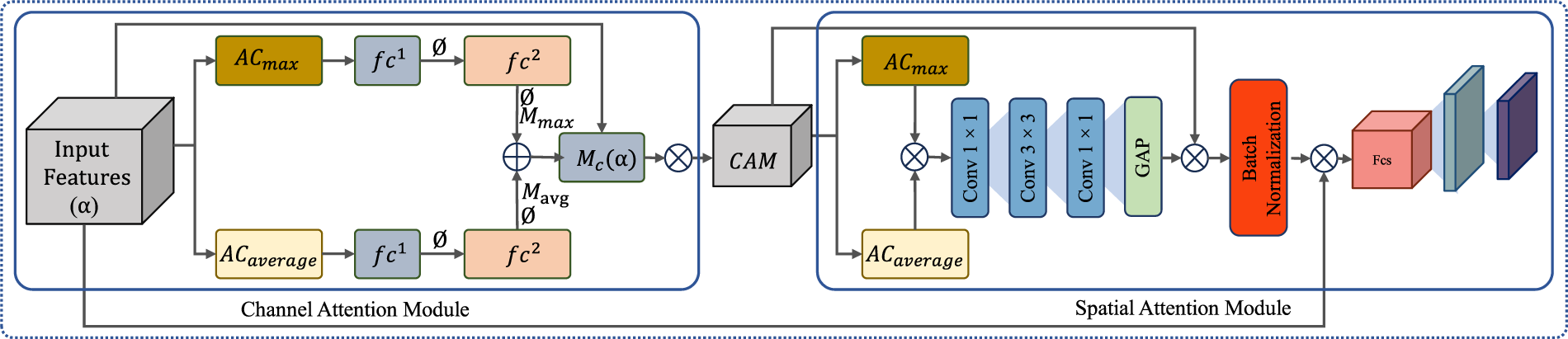
Figure 3: General overview of the attention mechanism.

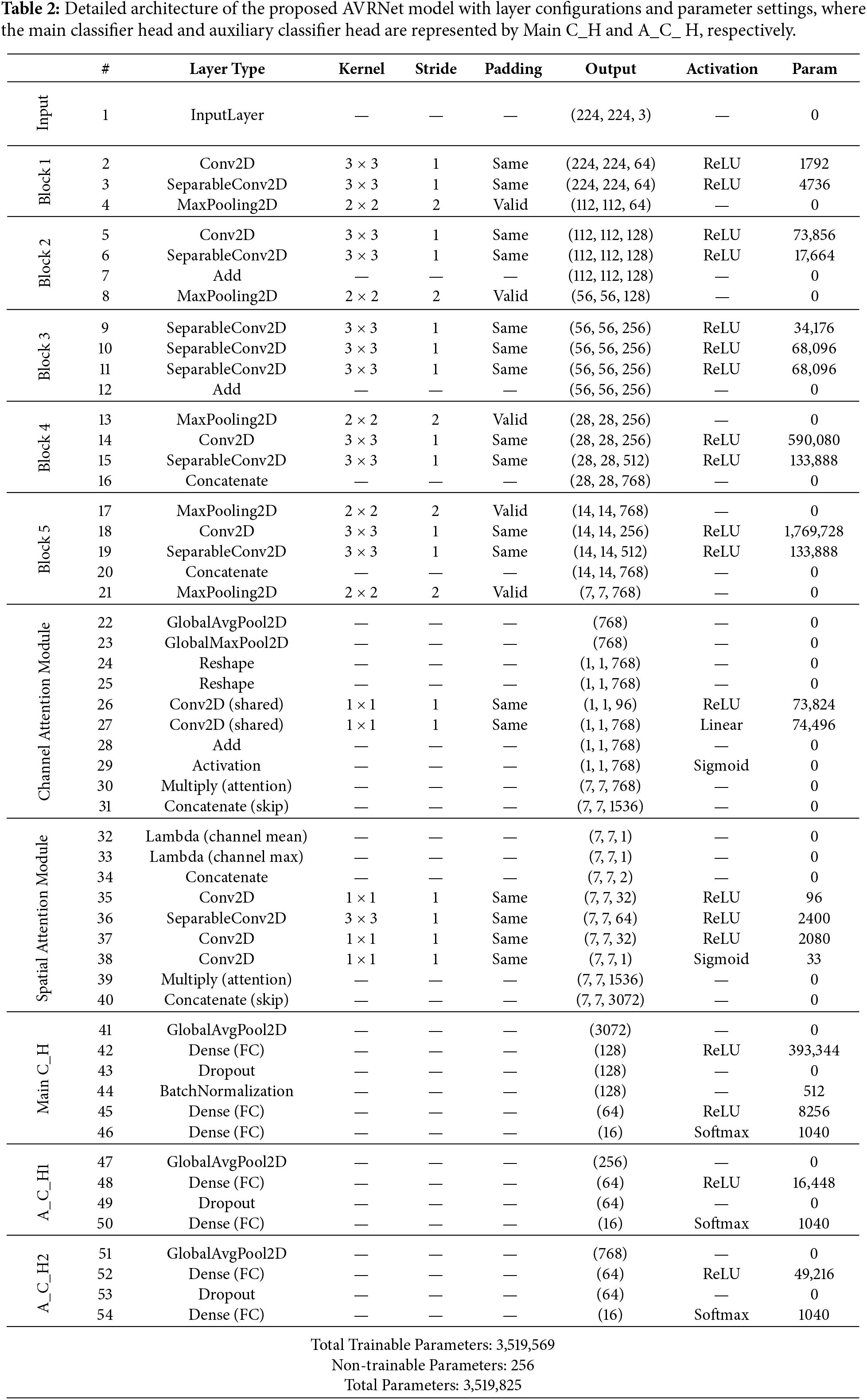
Table 2 summarizes the complete architecture of the proposed AVRNet model. The proposed network consists of five convolutional feature extraction blocks integrated with modified channel and spatial attention mechanisms, along with auxiliary classifiers for hierarchical deep supervision. Overall, the proposed AVRNet contains approximately 3.51 million trainable parameters, providing an effective balance between classification performance and computational efficiency.

3  Experimental Results

The proposed AVRNet model was experimented on a 13th Generation Intel Core™ i7 CPU operating at 2.60 GHz with 24 GB of RAM, with additional support of an NVIDIA GeForce RTX 4060 GPU having 8 GB VRAM, providing sufficient computational capability to train the deep learning models. The system runs on Windows 11; the implementation employed TensorFlow 2.10 as the back-end and Keras as a front-end framework, chosen for their efficiency and GPU acceleration support. Several supporting libraries were also utilized, including Pandas and NumPy for data manipulation, Scikit-learn for dataset splitting, stratified partitioning, and performance evaluation, and Matplotlib for result visualization. To ensure full reproducibility across all experiments, the model was trained using the Stochastic Gradient Descent (SGD) optimizer with a learning rate of 0.0001 and momentum of 0.9, and a batch size of 8 over a maximum of 100 epochs. To prevent overfitting and reduce unnecessary computation, an EarlyStopping callback was employed with a patience of 20 epochs, monitoring validation accuracy and automatically restoring the best model weights upon termination. In addition, a ModelCheckpoint callback was configured to save the best-performing model based on the highest validation accuracy achieved during training, enabling reliable post-training evaluation and fine-tuning. The hyperparameters were selected empirically based on validation-set performance, using multiple preliminary experiments to achieve stable convergence and improved generalization.

3.1 Evaluation Parameters

In this subsection, the evaluation metrics used to assess the proposed model are defined. Accuracy is the overall recognition rate, computed as the ratio of correctly classified samples to the total number of samples:

Accuracy=TP+TNTP+TN+FP+FN(17)

Precision is the ratio of correctly classified positive samples to the total number of samples predicted as positive. A high precision indicates that the model rarely produces false positives, as computed below:

Precision=TPTP+FP(18)

Recall is the ratio of correctly classified positive samples to the total number of actual positive samples; a high recall indicates that the model rarely misses positive instances, as computed with Eq. (19).

Recall=TPTP+FN(19)

The F1-score is the harmonic mean of precision and recall, providing a single balanced summary. These metrics are formally defined in Eq. (20)

F1−score=2×Precision×RecallPrecision+Recall(20)

3.2 Dataset Information

This subsection provides an explanation of the datasets used in the proposed work implementation. The proposed model is evaluated using two different datasets, such as EmreSasmaz [18], and the proposed custom dataset.

3.2.1 EmreSasmaz Dataset

This dataset consists of ten different animal voices in .wav sound format from various internet sources. To ensure that the voice recordings were clean, the audio files were collected into 1050 pieces, each of which was manually examined to avoid errors. The size of each file was set to at least 3 KB, and if the size was less than the specified threshold, the data could not be processed. Their final dataset consisted of 875 voices of 10 different animals, including birds, cats, chickens, cows, dogs, donkeys, frogs, lions, monkeys, and sheep [18]. The number of samples per class is given in Fig. 4. The dataset size is small, and some of the classes have very few training examples, which increases the chances of model overfitting and reduces robustness. Therefore, Sisodia et al. [36] applied data augmentation techniques to the EmreSasmaz dataset. To improve the model robustness and reduce overfitting, we employed the same data augmentation strategy previously used by Sisodia et al. [36] for animal vocalization recognition on the EmreSasmaz dataset. During training, additional samples were generated from the original audio recordings using additive white noise, time stretching, time shifting (rolling), and pitch shifting, as explained in [37]. Additive noise simulates real-world environmental disturbances, while time stretching modifies the playback speed without altering the signal content. Time shifting changes the temporal position of the audio signal, and pitch shifting adjusts the frequency characteristics of the vocalization. For a fair comparison with Sisodia et al. [36], the same augmentation techniques were applied in all experiments conducted on the EmreSasmaz dataset. The augmentation parameters were applied on complete dataset and fixed as a noise factor of 0.005, time stretching rate of 0.8, pitch shifting of ±2 semitones, and time shifting of 10% of signal length. These transformations were designed to simulate realistic acoustic variations while preserving the semantic content of animal vocalizations. Experiments on the EmreSasmaz dataset followed the original protocol of [18]: 80% training and 20% testing, with no separate validation set (early stopping monitored the training-set behaviour). This split matches the published baseline so that our EmreSasmaz numbers are directly comparable to prior work.

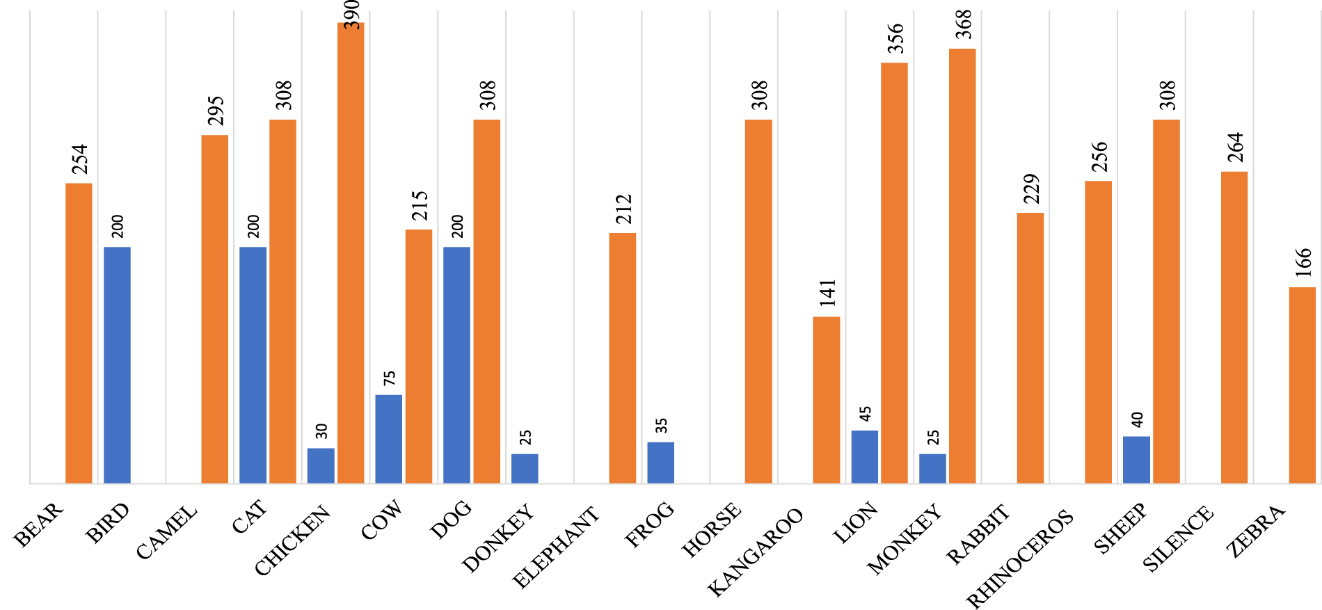
Figure 4: Distribution of samples in each class of the two datasets considered here: the blue bar represents EmreSasmaz (10 classes), and the orange bar shows the proposed dataset (16 classes).

3.2.2 The Proposed Dataset

A new animal vocalization dataset was developed for this study using audio recordings collected from both real-world environments and publicly available online multimedia sources. The dataset contains vocalizations from 15 animal classes, namely cats, dogs, horses, sheep, cows, elephants, bears, zebras, lions, monkeys, rhinoceroses, kangaroos, camels, chickens, and rabbits. In addition, a separate Silence/Noise class was incorporated to represent environmental background noise, silent intervals, wind noise, and sensor artefacts that may occur in practical acoustic monitoring scenarios where no animal vocalization is present. The inclusion of this class improves the robustness of the proposed model by reducing confusion between animal sounds and non-vocal acoustic events.

The dataset was constructed using recordings collected locally from real environments in Pakistan as well as publicly accessible online sources, including YouTube, Facebook, National Geographic documentaries, publicly available animal sound datasets such as the EmreSasmaz dataset, and other online audio resources. This multi-source collection strategy was adopted to increase acoustic diversity and improve the generalization capability of the model under varying environmental and recording conditions. Overall, the dataset contains 4378 audio clips distributed across 16 classes. The source-wise distribution of the collected samples is illustrated in Fig. 5a. Approximately 38.2% of the samples were obtained from local field recordings, 37.7% from YouTube, 6.0% from other online resources, 6.0% from extracted silence/noise segments, 5.5% from the EmreSasmaz dataset, 4.2% from Facebook, and 2.4% from National Geographic sources, as shown in Fig. 5a. Similarly, in each class, the number of samples from each source is shown in Fig. 5b.

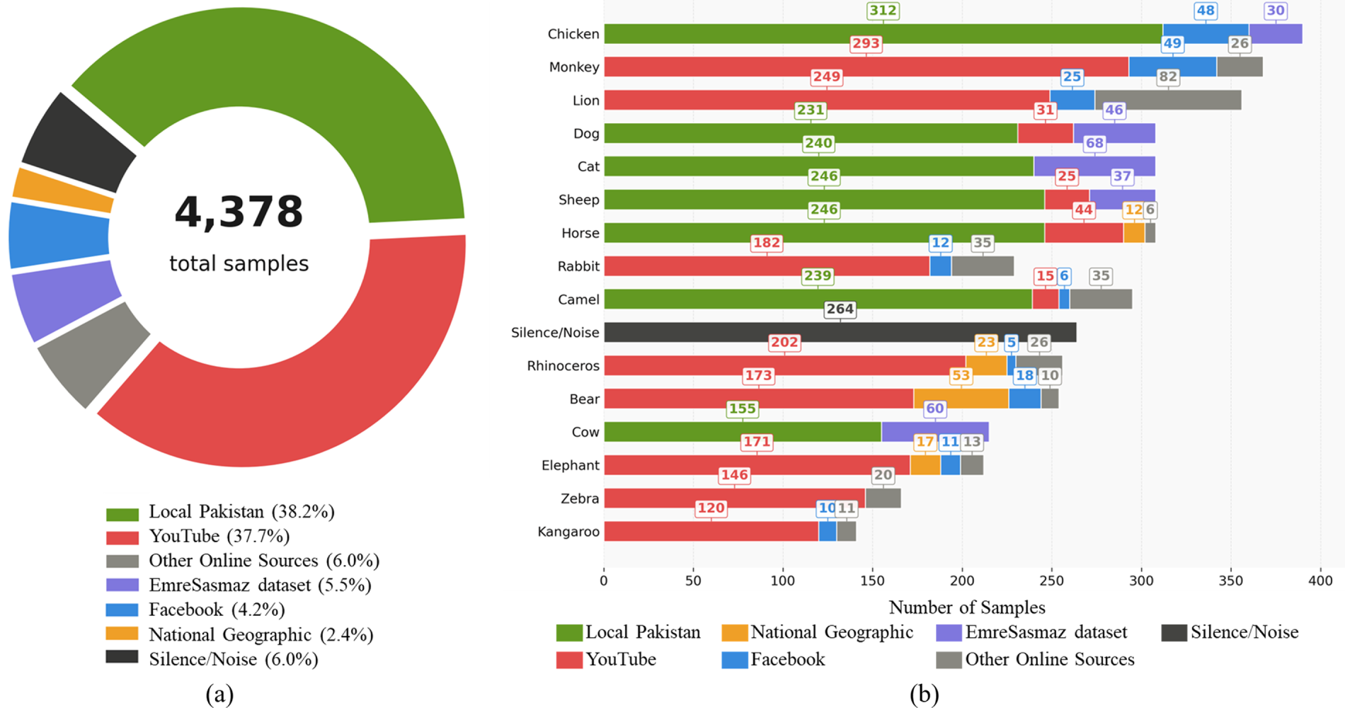
Figure 5: The proposed dataset collection information. (a) Total source distribution of the collected samples. (b) Class-wise source distribution illustrating the contribution of different sources across each category.

Dataset annotation was performed by three independent annotators with expertise in machine learning and audio signal analysis. The annotators included a PhD student from Gachon University (Republic of Korea), a Postdoctoral Researcher from Umeå University (Sweden), and a Postdoctoral Researcher from KAIST and Research Professor at Dongguk University (Republic of Korea). Following the source-wise partitioning procedure, recordings longer than 2 s were segmented into non-overlapping 2-s clips using Python audio-processing libraries (Librosa). This standardization ensured uniform temporal length across all samples prior to annotation. Each audio clip was independently reviewed through careful listening using the VideoLAN Client (VLC) media player. The annotators followed a consistent labeling guideline in which each clip was assigned to a single prevalent class based on the most prominent acoustic content. Clips containing multiple simultaneously vocalizing animal species, clips without identifiable animal vocalizations, and clips dominated by environmental/background sounds were separated during the initial screening stage. Following this process, the final dataset was organized into 16 classes, consisting of 15 animal vocalization categories and one additional noise class. The noise class included silence segments, environmental sounds, and recordings without identifiable target animal vocalizations. To ensure labeling consistency and reduce subjective bias, a cross-checking annotation strategy was adopted. After the initial labeling phase, each annotator independently reviewed and verified the labels assigned by the other annotators by re-listening to the corresponding audio clips. Any disagreements were resolved through discussion and consensus among all annotators before finalizing the dataset.

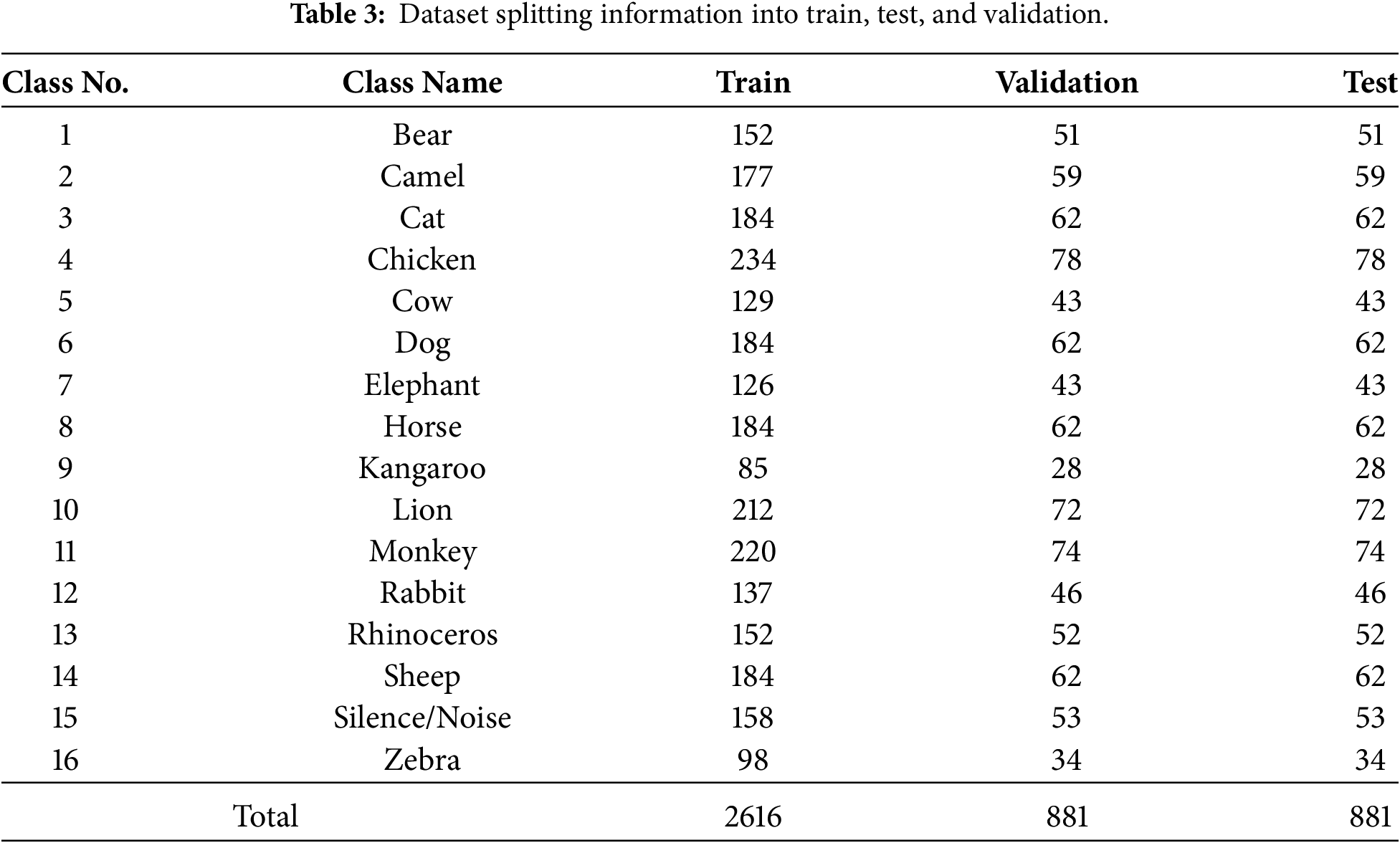
The annotation process was conducted manually after source-level partitioning and segmentation, with each audio clip assigned to the dominant animal vocalization category present in the recording. Annotation consistency was verified through repeated listening and cross-checking during preprocessing to minimize labelling inconsistencies. The source-recording-level partitioning ensured that all recordings were assigned exclusively to the training, validation, or test subset before clip segmentation. Consequently, clips originating from the same original recording, source video, or continuous recording session were not distributed across multiple subsets. This source-independent splitting strategy prevents data leakage and avoids overly optimistic performance estimates caused by acoustic similarities between training and testing samples. To ensure a fair evaluation, a subset of the source recordings was retained to maintain a 60%, 20%, and 20% distribution across the training, validation, and test sets, respectively (Table 3). The validation set was used exclusively for early stopping and best-checkpoint selection during training. The test set was held out completely and was used only once, for the final reported metrics; validation and test are strictly disjoint at both the clip level and the source-recording level. Since the AVR dataset was compiled from multiple heterogeneous sources, including local field recordings and publicly available online recordings, source-specific characteristics such as microphone response, compression artifacts, recording devices, and environmental conditions may introduce source-related bias. To mitigate this effect, recordings for each animal class were intentionally collected from multiple independent sources rather than relying on a single source, as illustrated in Fig. 5b. Furthermore, the source-recording-level partitioning was performed before segmentation, preventing clips from the same original recording from appearing in different subsets. Although these measures help reduce source-specific bias, they may not completely eliminate its influence on model performance.

3.3 Quantitative Results

This subsection provides a concise overview of the performance of AVRNet for efficient AVR. We conduct comparative analyses with the most prominent existing models on a benchmark dataset and a proposed custom dataset. This comparison aids in assessing the generalization capabilities of AVRNet in relation to other state-of-the-art models.

3.3.1 Experiments on the EmreSasmaz Dataset

Fig. 6 presents a detailed visualization of the confusion matrix, which provides a structured overview of the predictive accuracy of the model for each individual class within the classification task, thereby enabling a deeper understanding of the model’s strengths and potential areas for improvement. On the EmreSasmaz dataset, the Chicken, Frog, Lion, and Sheep classes exhibit comparatively lower recall than the remaining categories. These observations suggest that recognition errors mainly occur for classes exhibiting greater acoustic variability or overlapping spectro-temporal characteristics. Furthermore, the relatively small number of training samples available for several classes in the EmreSasmaz dataset increases the difficulty of learning robust class-specific representations.

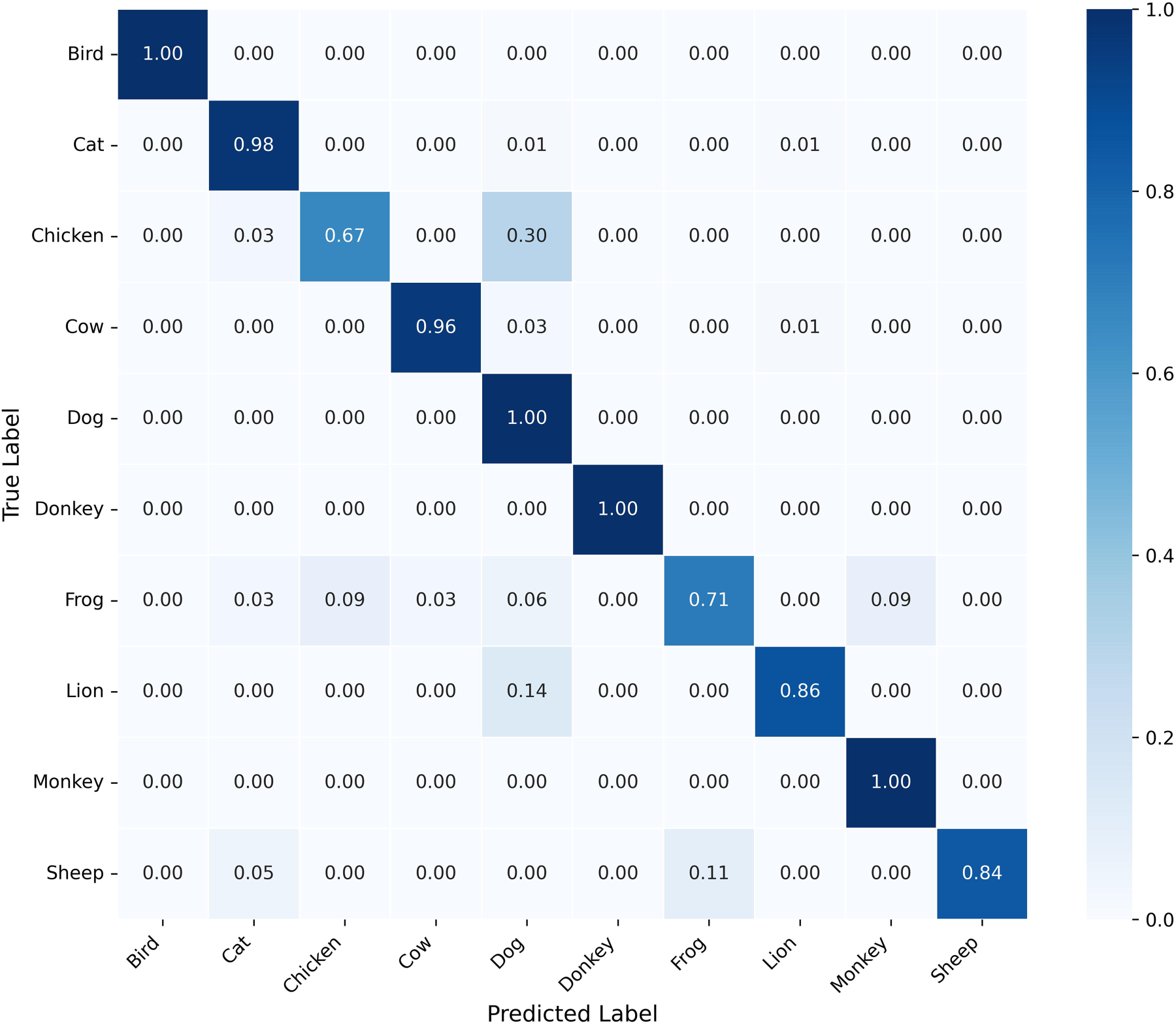
Figure 6: Confusion matrix of the proposed model on the EmreSasmaz dataset.

Table 4 presents a comprehensive assessment of AVRNet for AVR classification using the EmreSasmaz dataset. The recall, precision, F1-score, and accuracy metrics were used to gauge the efficiency of the proposed model. From Table 4, it can be seen that our model achieved higher precision for the classes of birds, donkeys, sheep, cows, cats, and lions; a lower precision was associated with the class of frogs and chickens, which reflects its competence in accurately identifying true positives among all the predicted positives. A high value for the precision indicates that the proposed model minimizes the occurrence of false positives. Likewise, the AVRNet achieved high values of recall for cows, dogs, birds, monkeys, and donkeys classes, although a lower recall was obtained for the chickens class. These results show that the AVRNet effectively captures and identifies a substantial proportion of actual positive cases in the dataset, with few false negatives. Table 4 shows that the AVRNet obtained higher F1 scores for the birds and Donkey classes, indicating a harmonious trade-off between recall and precision. This metric considers both false positives and negatives, enabling a holistic assessment of the model by considering its capability to find positive instances while reducing misclassifications. The proposed AVRNet model obtained an average accuracy of 95.53%.

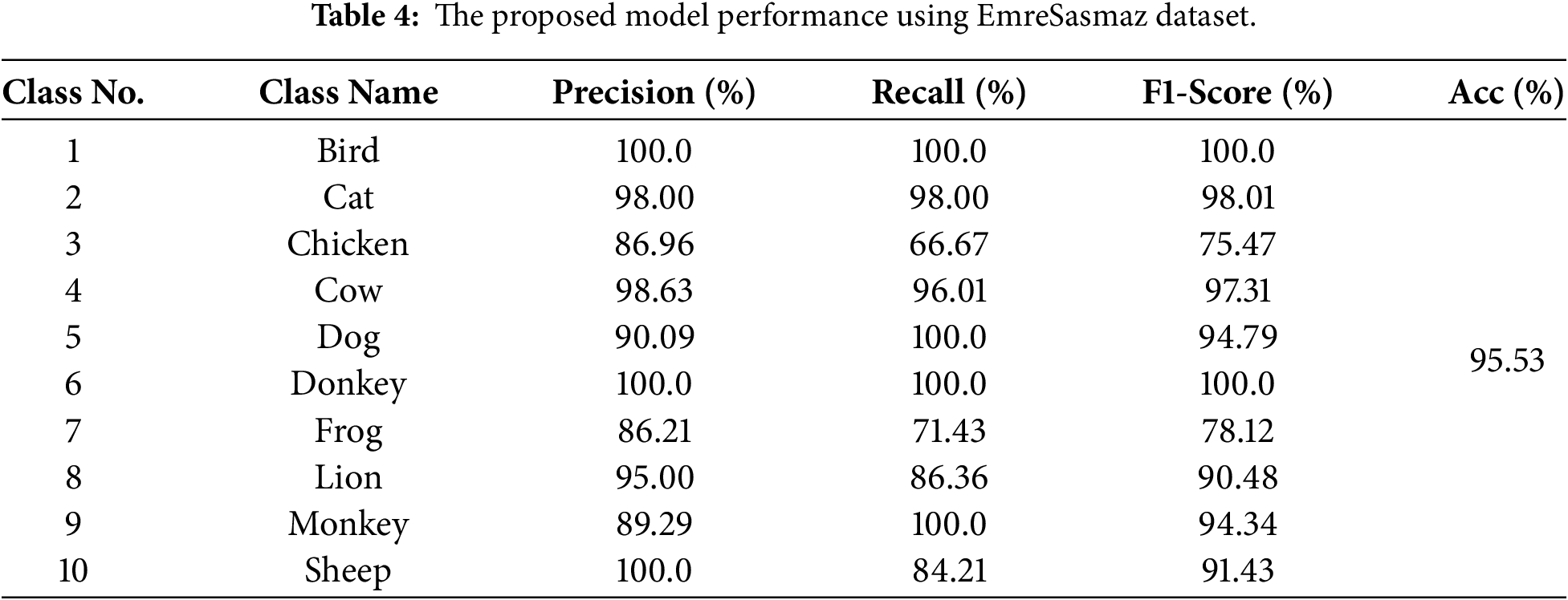
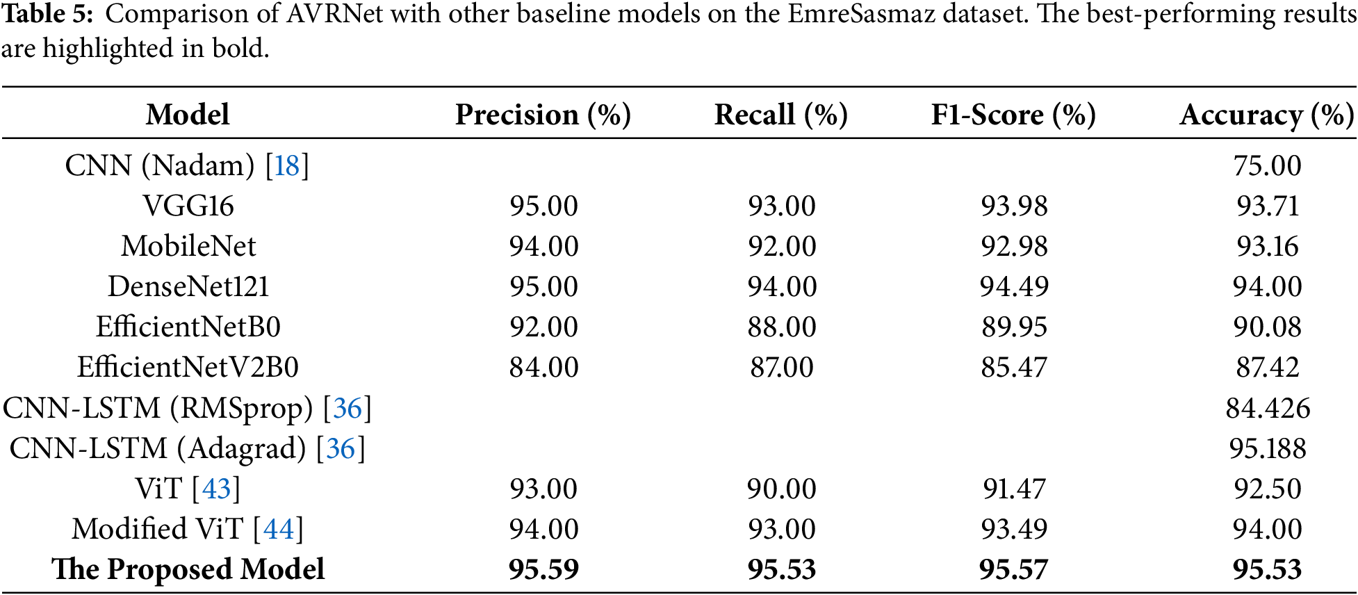
Table 5 shows the proposed model performance and its comparison with different deep learning models for AVR. The proposed AVRNet model obtained promising results using all evaluation parameters compared with several state-of-the-art deep learning models that had obtained promising results in other domains. In the comparative analysis, the proposed model surpassed the performance of VGG16 [38], MobileNet [39], DenseNet121 [40], EfficientNetB0 [41], and EfficientNetV2B0 [42] in terms of accuracy. The margins by which the proposed model outperformed these models were significant, with accuracy improvements of 1.82%, 2.37%, 1.53%, 5.45%, and 8.11% over VGG16, MobileNet, DenseNet121, EfficientNetB0, and EfficientNetV2B0, respectively. In the comparison as given in Table 5, the CNN (Nadam) [18] gave the worst results for the precision, recall, F1-score, and accuracy. Furthermore, Sisodia et al. [36] proposed a composite deep-learning model for animal voice recognition using the EmreSasmaz dataset. They used multiple strategies, combining a bidirectional long short-term memory (LSTM) network with a sequential convolutional neural network (CNN). Sisodia et al. [36] experimented with augmented and non-augmented EmreSasmaz datasets, using different model configurations and optimizers. In these methods, the CNN-LSTM(Adagrad) [36] obtained higher performance with 95.188% accuracy using an augmented dataset, and CNN-LSTM(RMSprop) [36] with 84.426% accuracy without an augmented dataset. However, the proposed model outperformed the CNN-LSTM (Adagrad) and CNN-LSTM (RMSprop), achieving accuracy improvements of 0.342% and 11.104%, respectively. Furthermore, the proposed research work reimplements the most recent methods, such as the Vision Transformer (ViT) proposed by Dosovitskiy [43] and a modified version of ViT proposed by Yar et al. [44] thereby, highlighting the proposed model’s effectiveness for animal voice recognition. The proposed model surpassed the Dosovitskiy [43], and Yar et al. [44] methods with better performance. These results indicate that AVRNet achieves the best overall performance across all evaluation metrics.

3.3.2 Experiments on the Proposed Dataset

Fig. 7 shows a detailed visualization of the confusion matrix, which provides a structured overview of the model’s predictive accuracy for each individual class within the classification task, thereby enabling a deeper understanding of the model’s strengths and possible areas for improvement.

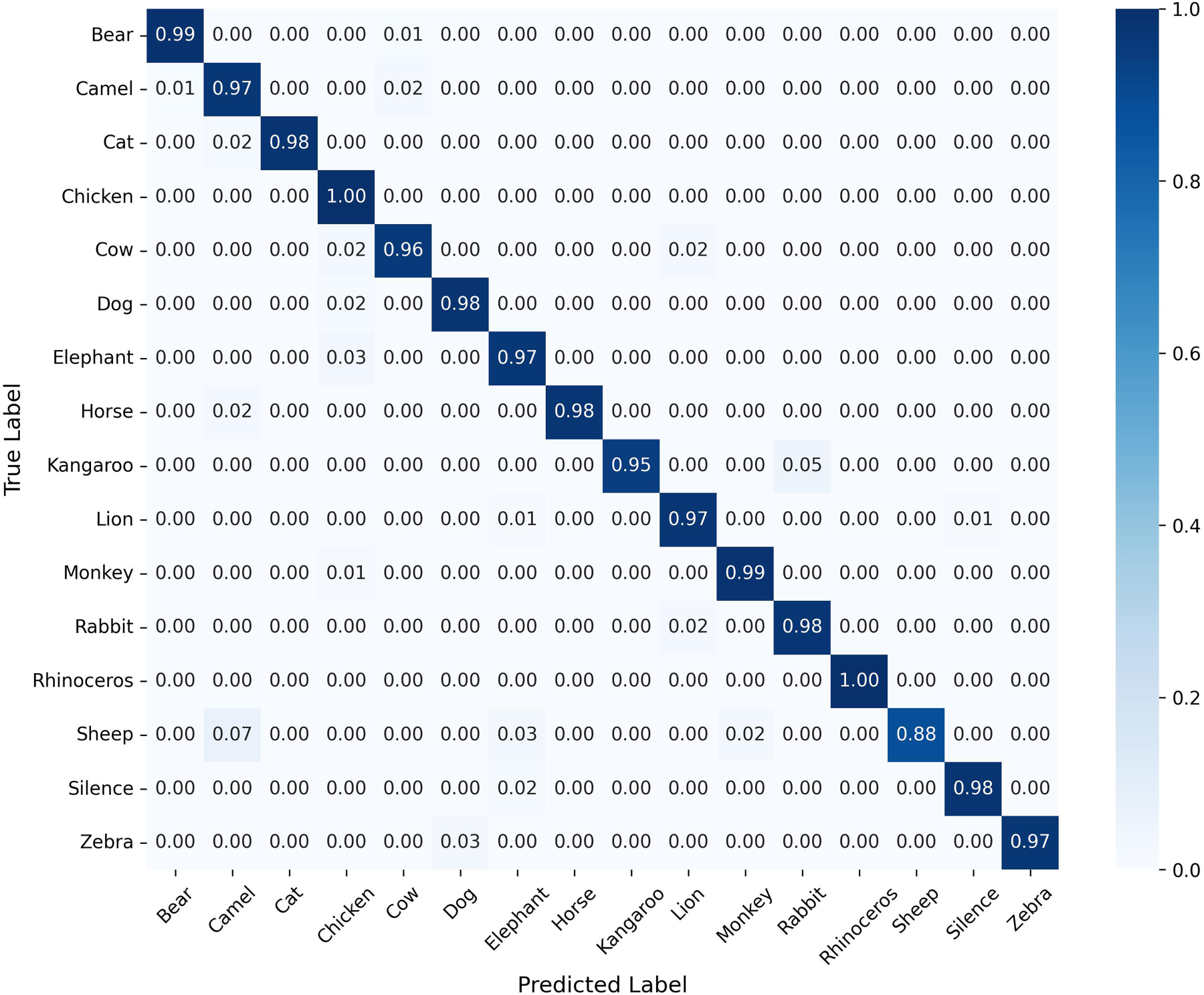
Figure 7: Confusion matrix for the proposed model on the newly developed dataset.

Table 6 shows the results for the proposed model on the newly developed dataset for AVR classification. The highest values of precision were found for the classes of bears, cats, dogs, horses, kangaroos, monkeys, rhinoceros, sheep, silence, and zebra classes, whereas the lowest precision was achieved for the class of camels. Likewise, higher values of the recall score were found for the classes of bears, camels, cats, chickens, dogs, elephant, horses, lions, monkeys, rabbits, rhinoceros, silence, and zebra whereas the lowest recall was seen for the sheep class. From Table 6, it can be seen that higher F1-scores were achieved for the classes of bears, cats, and rhinoceros, ranging from 99%–100%, representing a harmonious trade-off between precision and recall. The proposed model achieved an average accuracy rate of 97.19%.

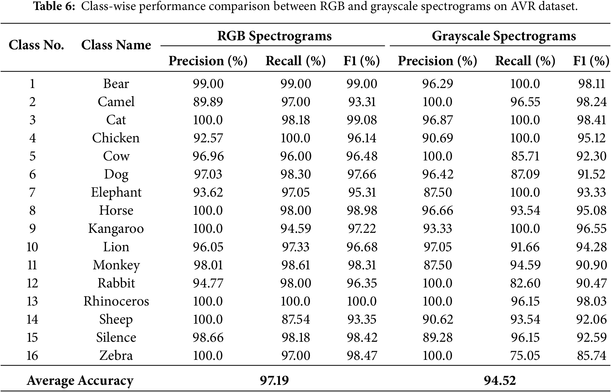
To justify the choice of RGB colormap spectrograms as the input representation for AVRNet, we performed an additional comparative experiment against grayscale spectrograms on the same dataset. Both representations are derived from the same underlying log-mel spectrogram of the audio signal: the RGB representation applies a perceptually non-linear colormap to encode the log-mel energy values across three channels, while the grayscale representation retains the raw log-mel spectrogram as a single-channel intensity image. Table 6 reports the class-wise Precision, Recall, and F1-score obtained using both representations. As shown in Table 6, the RGB colormap spectrogram consistently outperforms the grayscale spectrogram across most classes, achieving an average accuracy of 97.19% compared to 94.52% for the grayscale representation, a margin of 2.67%. Notably, the classes of Sheep, Rabbit, and Zebra, which contain acoustically overlapping or closely-spaced frequency components, show a considerably lower F1-score under the grayscale representation (92.06%, 90.47%, and 85.74%, respectively) compared to the RGB representation of Sheep, Rabbit, and Zebra (93.35, 96.35, and 98.47, respectively). This suggests that colormap encoding enhances the visual separability of subtle spectral energy variations that are otherwise compressed in a single-channel grayscale image, enabling the convolutional layers of AVRNet to extract more discriminative texture and edge information. Furthermore, since AVRNet’s backbone follows a standard CNN design optimized for three-channel inputs, the RGB representation allows extensive utilization of the network’s feature-extraction capacity relative to the grayscale input. These findings confirm that the RGB colormap spectrogram is a more effective input representation for the proposed AVRNet framework, supporting its adoption throughout this study.

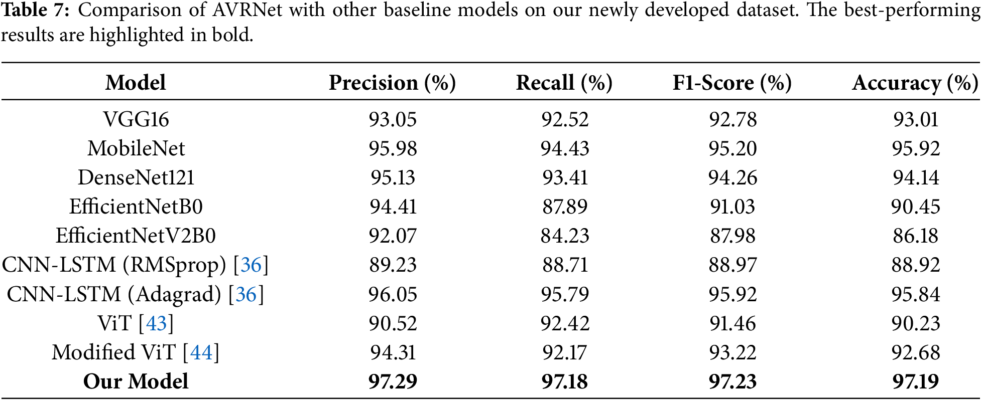
Table 7 compares the results of different deep learning models for AVR. The lowest performance in terms of the accuracy metric was achieved by EfficientNetV2B0, whereas the proposed model outperformed the other methods. In terms of average accuracy, our model achieved values that were 4.18%, 1.27%, 3.05%, 6.74%, and 11.01% higher than VGG16, MobileNet, DenseNet121, EfficientNetB0, and EfficientNetV2B0, respectively. Furthermore, the ViT [43] and a modified ViT [44] obtained an average accuracy of 90.23 and 92.68. The proposed model obtained 6.96% and 4.51% higher accuracy as compared to the ViT [43] and modified ViT [44], respectively. These results indicate that our model performs best across all evaluation metrics.

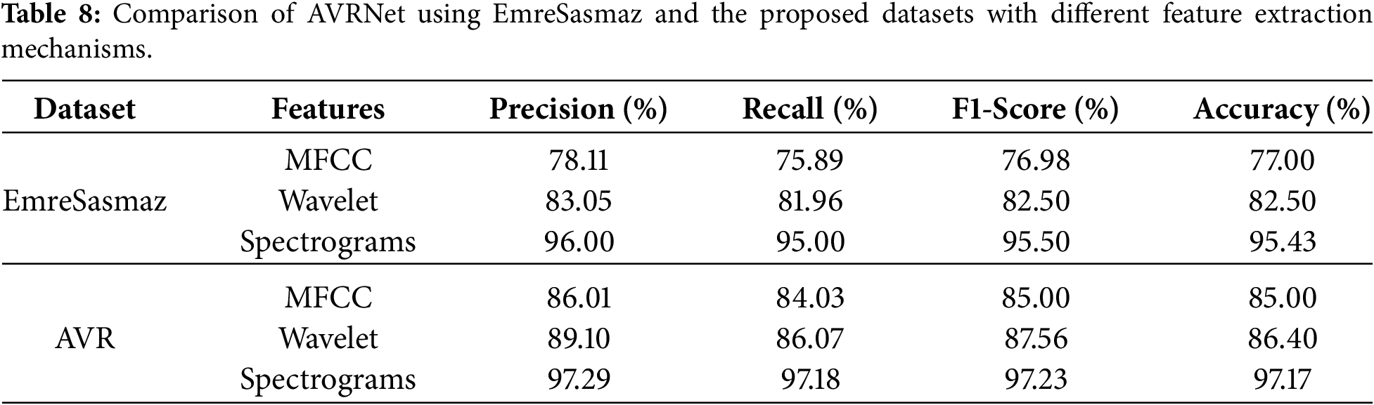
Furthermore, Table 8 shows the performance of the AVRNet on both the EmreSasmaz and the proposed datasets, using different feature extraction methods, including MFCC, wavelet, and spectrogram. The results indicate that the AVRNet trained on spectrogram features consistently achieved higher performance than other feature extraction techniques. On the EmreSasmaz dataset, the model trained with MFCC features obtained an average accuracy of 77.00%, which is 18.43% lower than the accuracy achieved with spectrogram features. Similarly, the model trained with spectrogram features achieved 12.93% higher accuracy than the model trained with wavelet features. For the proposed dataset, AVRNet trained with spectrogram features outperformed MFCC- and wavelet-based feature extraction methods, achieving 12.17% and 10.77% higher accuracy, respectively. These results demonstrate the superiority of spectrogram features in enhancing the performance of the AVRNet across different datasets.

3.4 Visualization

This section visualizes the model’s predictions in conjunction with each spectrogram image, as shown in Figs. 8 and 9. Fig. 8 shows a range of sample images that the proposed model predicted accurately. These include the classes of camels, cats, dogs, kangaroos, lions, rabbits, rhinoceros, and instances of silence. Despite this success, however, there are some cases where misclassification occurs due to the similarities between the features of classes within a given image, as given in Fig. 9. For example, the last images for the classes of bears, horses, monkeys, sheep, and zebras are misclassified. A bear is confused with a cow, a horse with a camel, a monkey with a chicken, a sheep with a camel, and a zebra with a dog. The confusion between bears and cows could be due to various factors, even though the vocalizations of these two animals are generally distinct. For example, both animals may produce low-frequency sounds with similar features, such as low-pitched growling or rumbling. In the scenario of a horse and a camel, both can exhibit a degree of flexibility in their sounds. Naturally, Horses can produce different forms of vocalization, including whinnies, neighs, and snorts, which can vary in pitch and intensity. This irregularity occasionally results in the overlapping of the acoustic features. The individual variability or certain environmental factors affecting vocalizations might cause shallow relationships that the model finds challenging to differentiate, and this may cause confusion. Furthermore, if the training data contains examples in which each class’s spectrograms are acoustically similar due to recording conditions or other factors, the model might struggle to distinguish between them. Class imbalance is also a factor affecting misclassification. Despite some misclassifications, our model produces promising results compared to the other models considered in our experiments.

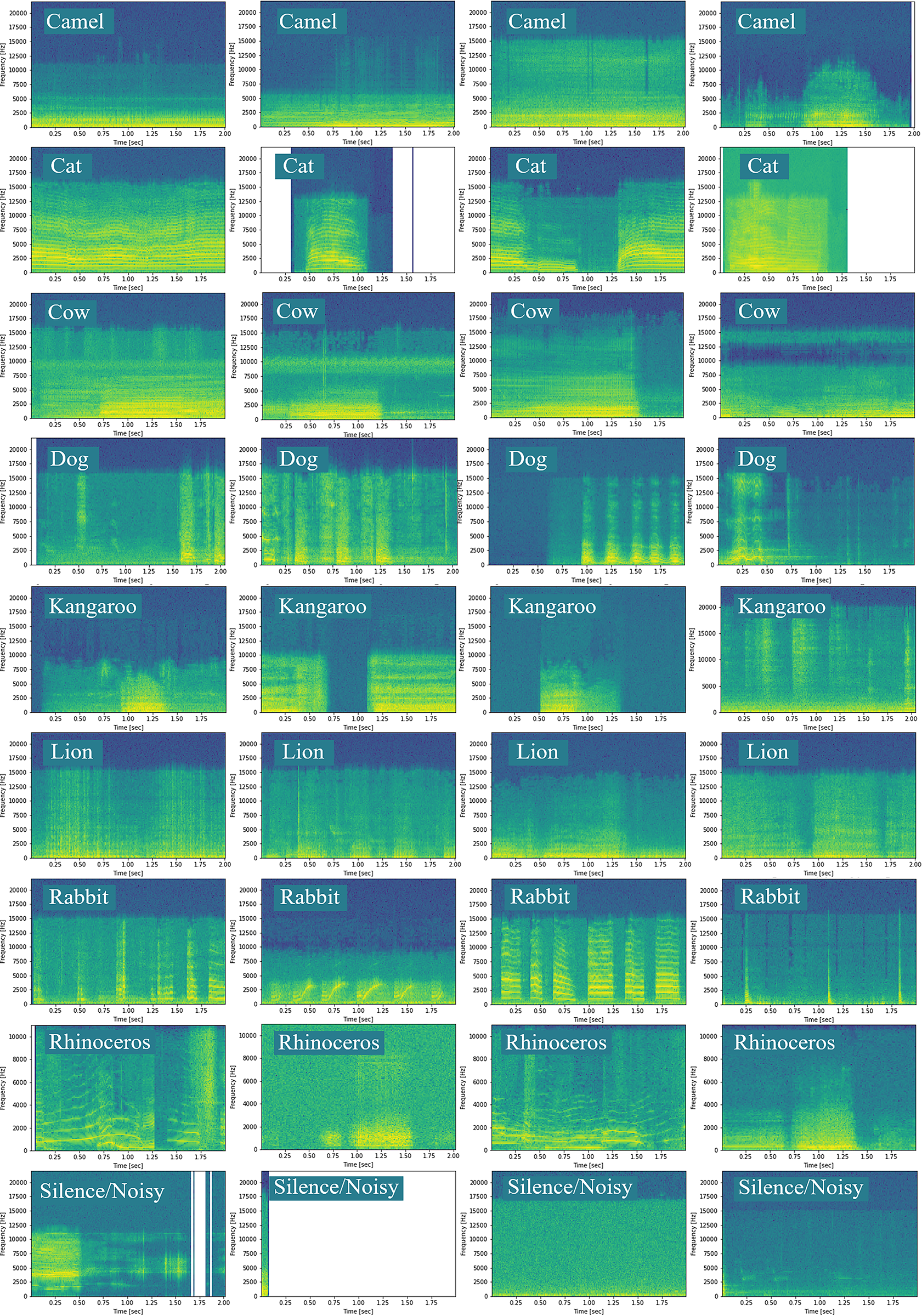
Figure 8: Results from the proposed model on the newly developed dataset.

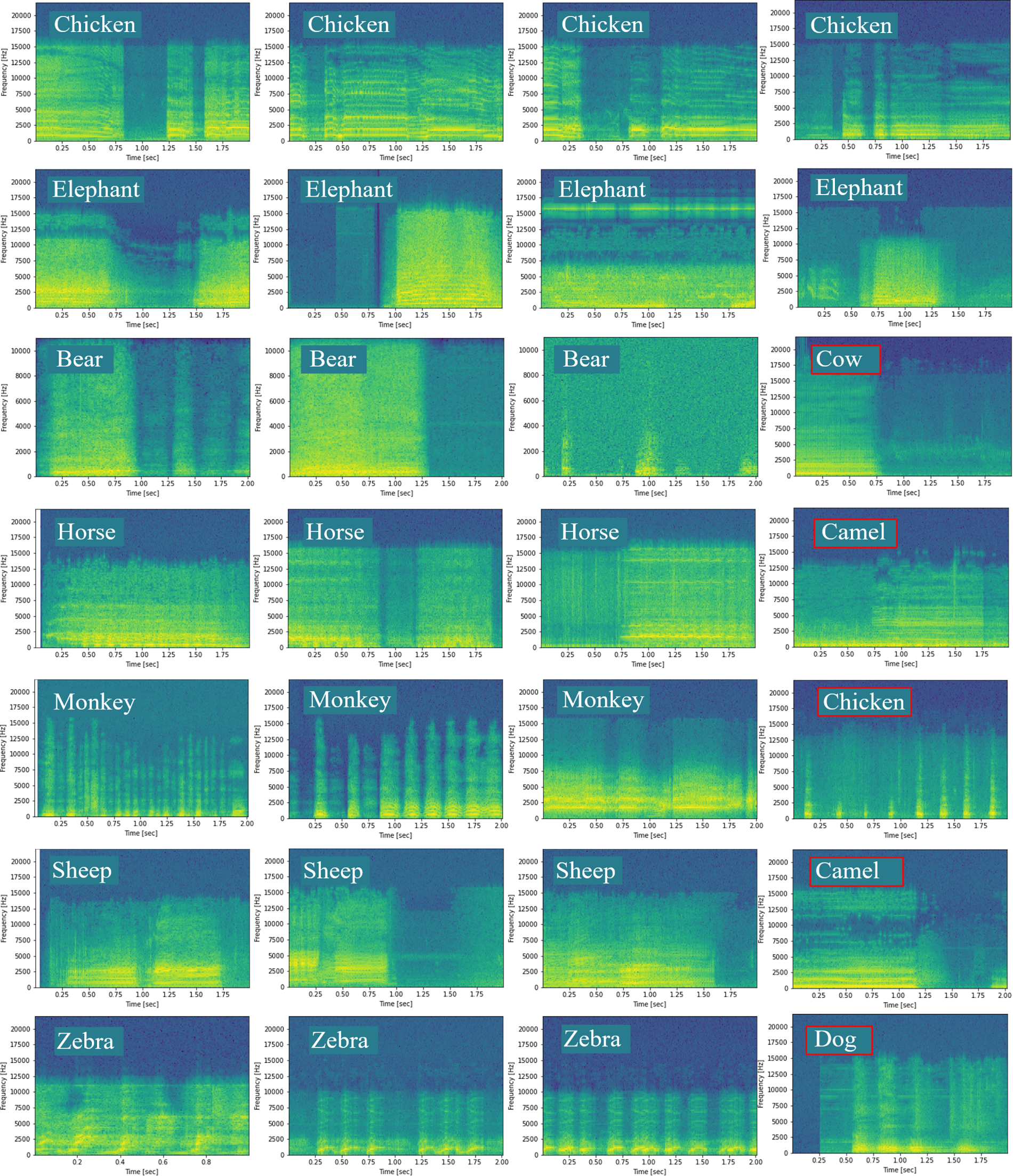
Figure 9: Results from the proposed model on the newly developed dataset with some misclassified samples.

3.5 Ablation Study of Our Model for AVR Classification

The objective of the ablation study is to evaluate the cumulative contribution of the principal architectural components integrated into AVRNet rather than to isolate the effect of every individual module independently. Consequently, each experiment progressively incorporates additional components to illustrate how the overall network evolves toward the final architecture, as shown in Table 9. Therefore, this strategy considers eight different variations. The initial experiment used only 2D convolutions, without incorporating other modules. This configuration involved 5.99 million learning parameters. In Experiment 2, only the skip connections were introduced to retain the information from the preceding layers. The use of this strategy substantially improved the model’s performance but increased the number of training parameters to 6.59 million. Experiment 3 applied a separable convolution operation in some layers instead of traditional convolutions to reduce the training parameters; however, the performance of the model was diminished compared to the previous experiments. Experiment 4 utilized traditional convolution along with separable convolutions, spatial attention, and a skip connection. This strategy improved the performance while giving a more efficient structure, with 3.17 million training parameters. Experiment 5 introduced channel attention instead of spatial attention, and the other network remains the same as experiment 4, which improved the performance compared to the previous experiment 4. In the next experiment, we introduced CBAM, which incorporated channel and spatial attention mechanisms, separable convolutions, and skip connections, achieving better the previous experiments as given in Table 9. Experiment 7 incorporated the CBAM (channel and spatial attention) mechanism along with auxiliary classifiers without separable convolutions, and achieved the best performance; however, it doubled the model complexity as compared with the proposed model. The final experiment incorporated modified CBAM (channel attention and spatial attention), separable convolutions, skip connections, and auxiliary classifiers. This arrangement obtained a better trade-off between model accuracy and computational complexity. As shown in Table 9, the progressive incorporation of separable convolutions, attention mechanisms, skip connections, and auxiliary supervision consistently improves the recognition performance. Although Experiment 7 achieves the highest classification performance, it requires approximately twice the number of learnable parameters compared with the proposed AVRNet architecture. In contrast, AVRNet achieves comparable recognition accuracy while reducing the model complexity by nearly 50%, demonstrating a more favorable balance between predictive performance and computational efficiency. Therefore, the proposed architecture was selected as the final model because it offers an effective trade-off between accuracy and computational complexity.

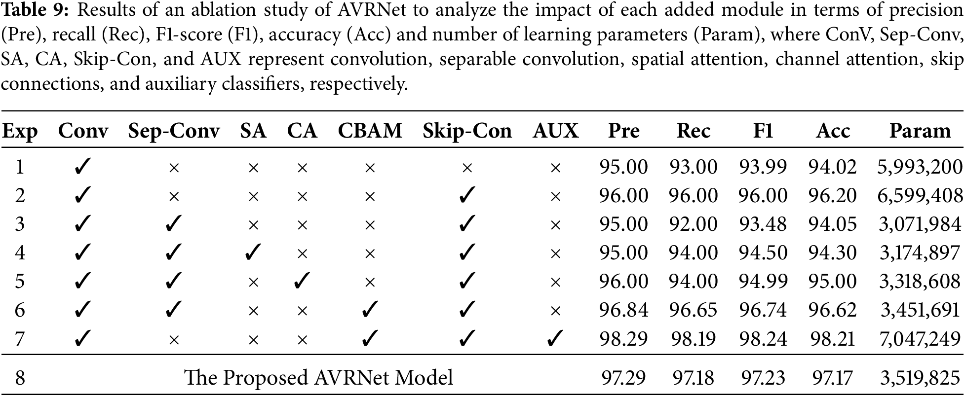
Furthermore, we investigated the effect of the auxiliary loss weights, and a sensitivity analysis was conducted using five different weight configurations while maintaining all other training parameters unchanged. The results are summarized in Table 10. The proposed weight configuration of (0.3, 0.2) achieved the highest performance on both datasets, yielding test accuracies of 98.46% and 96.11% on the AVR and EmreSasmaz datasets, respectively, together with the highest macro-F1 scores. Lower auxiliary weights did not provide sufficient intermediate supervision, whereas larger weights caused the auxiliary objectives to dominate the optimization process, resulting in a slight decrease in the final classification performance. These results indicate that the selected auxiliary loss weights provide an effective balance between the auxiliary branches and the primary classification objective, leading to improved optimization and generalization.

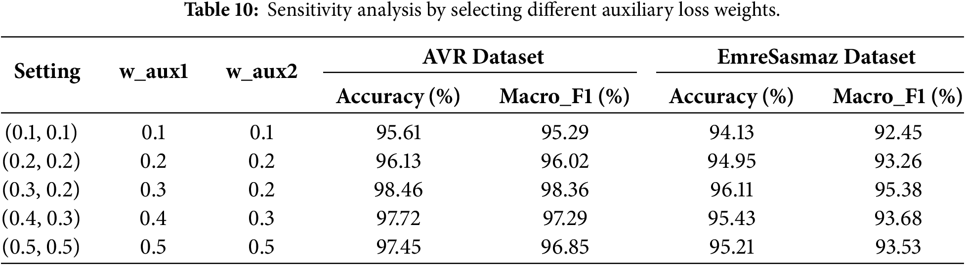
Fig. 10 presents the training convergence of the proposed AVRNet with and without the auxiliary classifiers on both datasets: panels (a, b) correspond to the EmreSasmaz dataset and panels (c, d) to the AVR dataset, reporting the training loss and training accuracy, respectively, over 100 epochs. All other architecture, hyper-parameters, optimizer, and data settings are identical between the two configurations, so any difference in the trajectories is attributable to the auxiliary classifiers. Across both datasets, the auxiliary classifiers produce a faster, lower, and significantly more stable optimization trajectory. On the EmreSasmaz dataset, the model with auxiliary classifiers reaches 95% training accuracy substantially earlier than the ablated model (epoch 57 vs. 71) and results in a lower training loss with less epoch-to-epoch fluctuation. The effect is even more obvious on the AVR dataset, where the ablated model exhibits large loss spikes and pronounced accuracy fluctuations throughout training, whereas the model with auxiliary classifiers converges smoothly to a low loss and stabilizes close to its final accuracy. In both cases, the final training loss is lower, and the final training accuracy is higher with the auxiliary classifiers than without them. This behavior is consistent with the role of deep supervision: the auxiliary classifiers inject supervisory gradients at intermediate layers, improving gradient flow through the network and producing faster and more stable convergence. These convergence and training-loss curves therefore provide direct evidence that the auxiliary classifiers improve the optimization of the network.

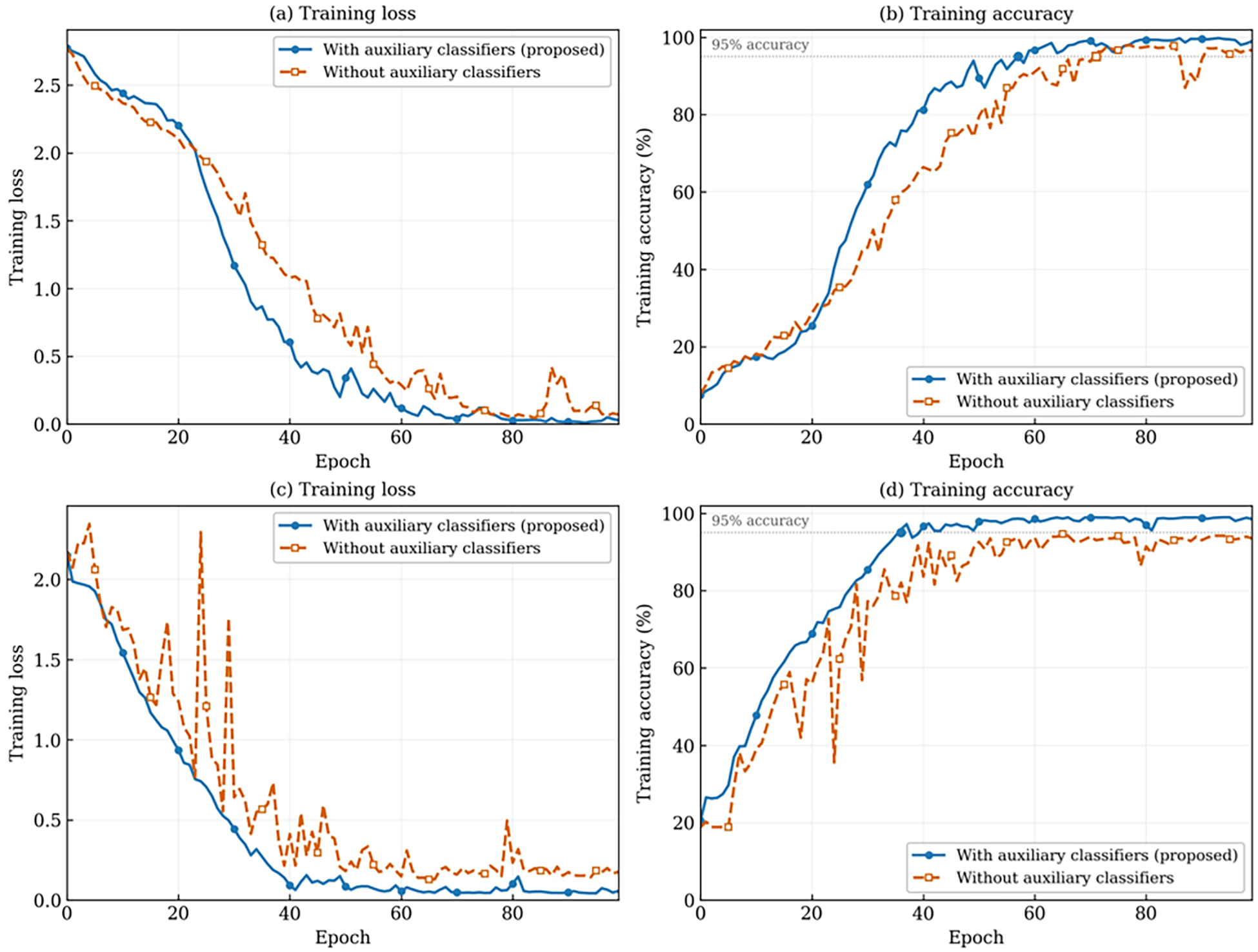
Figure 10: Effect of the auxiliary classifiers, shown for both datasets: (a,b) EmreSasmaz and (c,d) AVR.

3.6 Statistical Analysis

To evaluate the robustness and reproducibility of the proposed model, we performed two different experiments such as experiment with five different random seed selections using 42–46 and experiments with 5-Fold cross validation for a statistical significance test, as explained in the following subsections.

3.6.1 Performance Stability across Random Seeds

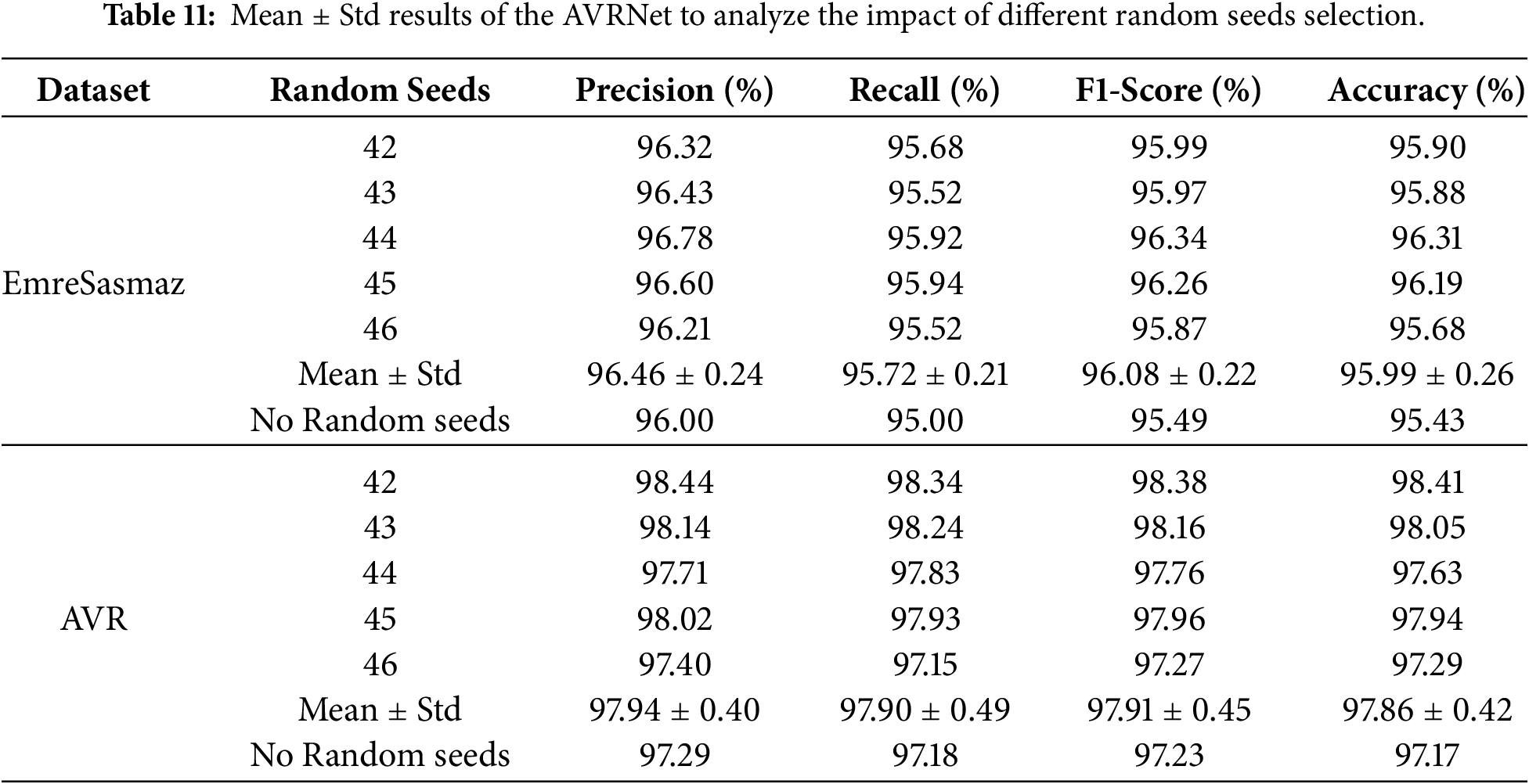
Table 11 shows the obtained results in terms of precision, recall, F1-score, and accuracy for both the EmreSasmaz dataset and the proposed dataset. In Table 11, it can be seen that the experiments were also performed without fixing a random seed, referred to as the “No Random Seeds” setting. These results represent the primary reported performance of the proposed framework. For the EmreSasmaz dataset, the proposed model achieved an average precision of 96.46 ± 0.24%, recall of 95.72 ± 0.21%, F1-score of 96.08 ± 0.22%, and accuracy of 95.99 ± 0.26% across different random seeds. Similarly, on the proposed dataset, the model achieved an average precision of 97.94 ± 0.40%, recall of 97.90 ± 0.49%, F1-score of 97.91 ± 0.45%, and accuracy of 97.86 ± 0.42%. The proposed model achieved the best performance with random seeds 44 and 42 over EmreSasmaz and the proposed datasets, respectively. The relatively low standard deviation values observed in both datasets indicate that the proposed model demonstrates stable and consistent performance under different random initializations.

3.6.2 Statistical Significance Test

To further validate the effectiveness and generalization capability of the proposed AVRNet model, a statistical significance test based on the paired t-test was conducted. The t-test is a statistical hypothesis test used to determine whether a significant difference exists between the means of two groups by computing a t-statistic and a corresponding p-value. The t-statistic measures the difference between the means of the two groups relative to the variability of the paired observations; a larger absolute value indicates that the two means differ more strongly in terms of the standard error. The p-value is the probability of obtaining a difference at least as large as the one observed, assuming the null hypothesis is true, where the null hypothesis states that the two models have equal mean accuracy. A significance level of 0.05 is adopted as the decision threshold: if the p-value is less than 0.05, the null hypothesis is rejected, and the difference between the two models is considered statistically significant.

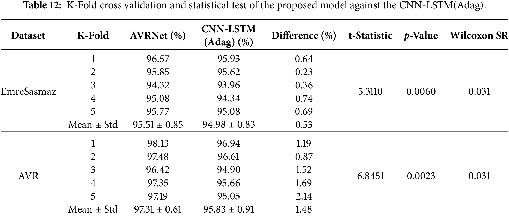
In this work, the paired t-test was applied to the accuracies obtained from five-fold cross-validation, pairing the proposed AVRNet with the strongest baseline, CNN-LSTM (Adagrad), on each fold. In the experiments, both models were evaluated on identical fold partitions; the paired formulation isolates the effect of the model from any variability introduced by the data splits. The test was performed independently on the EmreSasmaz dataset and the proposed AVR dataset; the per-fold accuracies, their mean ± standard deviation, the fold-wise differences, and the resulting t-statistics and p-values are reported in Table 12. On the EmreSasmaz dataset, AVRNet achieved an average accuracy of 95.51 ± 0.85%, and the CNN-LSTM (Adag) obtained an average accuracy of 94.98 ± 0.83%. The paired t-test produced a t-statistic of 5.3110 and a p-value of 0.0060, which is considerably lower than the significance threshold of 0.05. This confirms that the performance improvement achieved by AVRNet on the EmreSasmaz dataset is statistically significant. Similarly, on the AVR dataset, the proposed model outperformed CNN-LSTM (Adag) across all folds, obtained an average accuracy of 97.31 ± 0.61%, and the CNN-LSTM (Adag) model obtained an average accuracy of 95.83 ± 0.91%. The paired t-test yielded a t-statistic of 6.8451 and a p-value of 0.0023. Since the p-value is significantly below 0.05, the null hypothesis is rejected, indicating that AVRNet provides a statistically significant improvement over CNN-LSTM (Adag) on the AVR dataset. Furthermore, we investigated the improvements of AVRNet over the strongest baseline (CNN-LSTM optimized with Adagrad), which are statistically significant without assuming normally distributed differences. We complemented the paired t-test with a non-parametric Wilcoxon signed-rank test applied to the per-fold accuracies of the five-fold cross-validation. As summarized in Table 12, AVRNet achieved a higher accuracy than the baseline in every one of the five folds on both datasets, so the signed-rank statistic reached its most extreme value (W = 0). The corresponding one-sided p-value was 0.031 for the EmreSasmaz dataset (mean difference 0.53%) and 0.031 for the AVR dataset (mean difference 1.48%), indicating a statistically significant improvement at the 0.05 level in both cases. These non-parametric results agree with the parametric paired t-test and confirm that the performance gains of the proposed model are consistent across folds rather than the result of random variation.

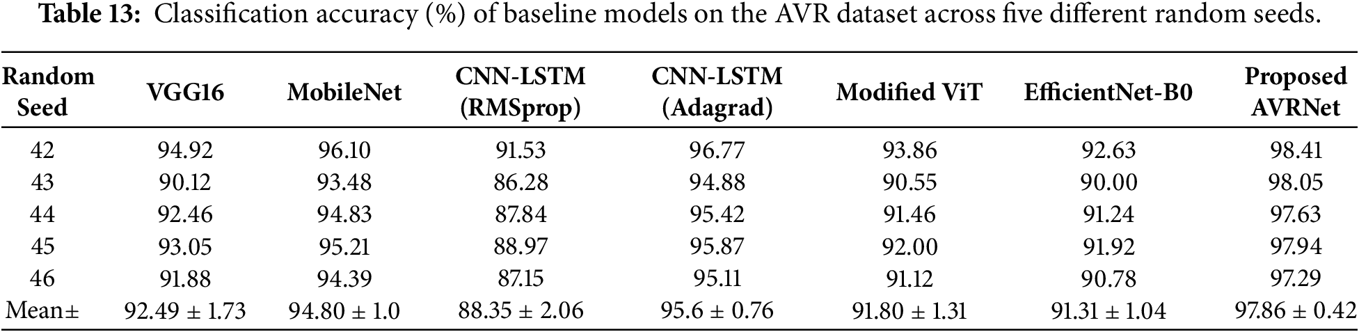
To further analyze the stability of each model and enable a fair comparison under identical conditions, every baseline and the proposed AVRNet were trained and evaluated over five independent runs on the AVR dataset, using different random seeds. Table 13 reports the per-run accuracy together with the mean and sample standard deviation over the five runs for all models. The proposed AVRNet attains the highest mean accuracy (97.86%) and, simultaneously, the smallest standard deviation (±0.42), indicating that the proposed model is a suitable choice for the targeted domain. Among the baselines, CNN-LSTM with the Adagrad optimizer is the strongest (95.61 ± 0.75), followed by MobileNet (94.80 ± 0.97) and VGG16 (92.49 ± 1.73), while the CNN-LSTM model trained with RMSprop shows both the lowest mean accuracy and the largest variability (88.35 ± 2.06). Overall, the proposed method improves the mean accuracy by 2.25 percentage points over the best-performing baseline while also reducing the run-to-run standard deviation, confirming that its reported performance is consistent rather than the outcome of a single favorable run.

3.7 Complexity Analysis

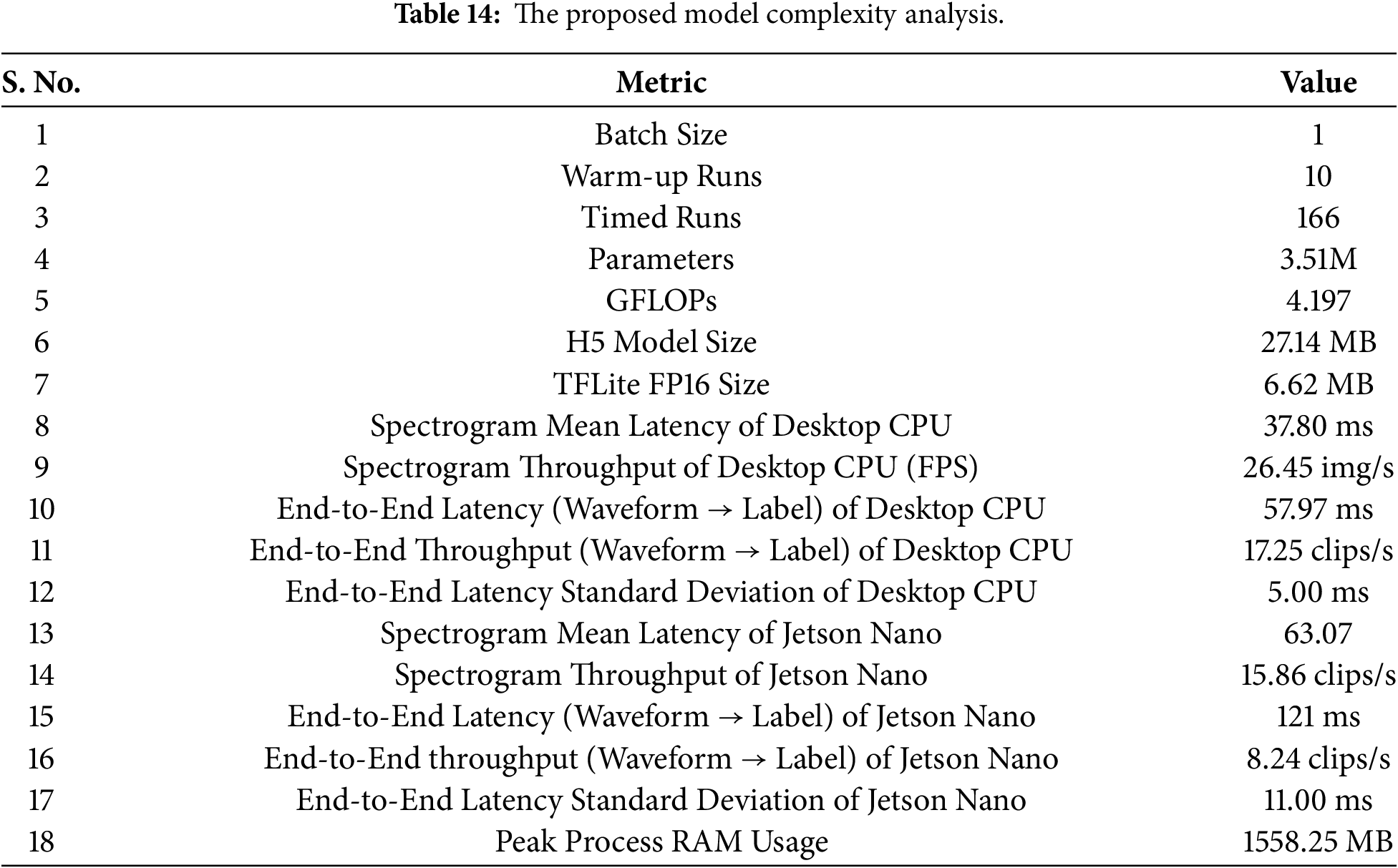
To further evaluate the computational efficiency of the proposed framework, a desktop CPU and NVIDIA Jetson Nano-based inference analysis was conducted. Before recording the measurements, 10 warm-up runs were performed to eliminate initialization overhead. The benchmark was then conducted on 166 audio clips using a batch size of one, and the reported latency corresponds to only the spectrogram classification and a complete end-to-end processing pipeline from waveform input to predicted class label. The proposed model contains approximately 3.51 million parameters with a computational complexity of 4.197 GFLOPs, and a model size of 27.14 MB, as given in Table 14. Experimental evaluation demonstrated an average inference latency of 37.80 ms per spectrogram image and a throughput of 26.45 images per second under CPU-only execution. The complete end-to-end waveform-to-label latency, covering audio loading, STFT computation, spectrogram rendering, resizing, normalization, and inference. All measurements use a batch size of 1, reflecting the single-clip nature of real-time monitoring. On the desktop CPU, AVRNet achieved an end-to-end latency of 57.97 ms (17.25 clips/s). To assess the feasibility on an embedded platform, the complete pipeline was deployed on an NVIDIA Jetson Nano (quad-core ARM Cortex-A57 CPU at 1.43 GHz, 128-core Maxwell GPU at 0.92 GHz, 4 GB shared LPDDR4 memory, Ubuntu 18.04 with CUDA 10.2, cuDNN 8, and TensorFlow 2.4.1), with inference executed on the Jetson GPU. The AVRNet achieved a mean end-to-end latency of 121.30 ms, corresponding to a throughput of 8.24 clips/s, demonstrating the practicality of AVRNet for on-device acoustic monitoring. Additionally, the trained model was converted into TensorFlow Lite (TFLite) formats to assess deployment feasibility on resource-constrained platforms. The FP16 TFLite model reduced the storage requirement to only 6.62 MB, demonstrating the suitability of the proposed framework for edge-device and embedded deployment scenarios. The low latency variation observed across benchmark runs further confirms the stability and practical applicability of the proposed architecture for intelligent audio classification systems. The reported peak process RAM of 1558.25 MB reflects the full Python-based inference environment (interpreter, TensorFlow/TFLite runtime, and imported libraries) rather than the model itself, which occupies only 6.62 MB in FP16 TFLite form. The current deployment envelope of AVRNet is therefore edge-class devices with ≥2 GB of memory, such as the NVIDIA Jetson Nano (4 GB), Raspberry Pi 4 (2–8 GB), and comparable single-board computers, but it exceeds the memory available on ultra-low-power microcontroller platforms (e.g., ARM Cortex-M-class devices). Deployment on such platforms would require additional compression techniques, INT8 quantisation, structured pruning, or knowledge distillation into a smaller student network.

4  Discussion and Implications

This research contributes both theoretically and practically to the field of AVR. The following points highlight the distinctive aspects and implications of our work.

4.1 Theoretical Contributions

4.1.1 Task-Specific Model Architecture

The proposed AVRNet model is a task-specific CNN architecture based on depthwise-separable convolutions, which foster a more resource-efficient learning process with fewer parameters and lower computational complexity. The multiscale feature extraction mechanism improves the model’s adaptability to objects of varying sizes, thereby enhancing its robustness when analyzing animal vocalizations of different durations, represented as 2D spectrograms. Furthermore, the integration of a modified attention mechanism enables the model to focus on critical regions in spectrograms, enabling more precise and discriminative species recognition. This configuration offers a favorable accuracy–efficiency trade-off relative to strong image-classification backbones, while being explicitly designed for spectrogram-based vocalization recognition.

4.1.2 2D Voice Signal Representation

The proposed model utilizes STFT-based spectrograms as the input representation for voice classification. STFT is a well-established signal processing technique that transforms raw audio signals into 2D time–frequency spectrograms, providing, representing signal intensity across different frequencies over time. This representation facilitates the extraction of rich and salient features from audio signals, enabling AVRNet to learn robust feature representations and improve classification performance. The novelty of the proposed approach lies in the AVRNet architecture and its effective exploitation of STFT-based spectrogram representations, rather than in the STFT transformation itself.

4.2 Practical Implications

4.2.1 Enhanced Species Identification

AVRNet’s state-of-the-art performance in species identification reflects its remarkable ability to distinguish between and categorize various animal species based on their vocalizations. As it achieves high levels of accuracy and efficiency across both datasets, AVRNet is shown to be applicable to real-world scenarios. This enhanced species identification capability is crucial for ecological studies, wildlife monitoring, and biodiversity conservation efforts. AVRNet’s precision in terms of recognizing distinct vocal patterns contributes significantly to the accurate classification of animal species and enables researchers to gather precise data for biodiversity assessments and ecological research. The proficiency of our model in species identification is not only a technological achievement but is also a valuable tool for advancing our understanding and conservation of diverse ecosystems.

4.2.2 Dataset Contribution

The impact of this study extends beyond the architecture of the AVRNet model and includes the development of a tailored dataset designed specifically for animal species recognition. This dataset addresses the limitations of existing datasets, which often focus on specific species, have limited numbers of instances for training, or lack a diverse range of vocalizations. The newly created dataset for AVRNet encompasses a diverse set of 15 animal species and accommodates class-level imbalances in the number of audio clips. It also includes a “silent/noisy class” for monitoring silent clips or background noise. This contribution not only enriches the available resources for researchers in the domain of animal voice recognition but also sets a standard for comprehensive and diverse datasets, fostering advancements in the field.

4.2.3 Efficiency in Wildlife Conservation

The practical implications of AVRNet are significant for wildlife conservation efforts. Accurate recognition of distinct animal species through vocalizations can serve as a powerful tool in monitoring and conservation initiatives. By deploying AVRNet on edge-class monitoring devices (Jetson Nano, Raspberry Pi 4, or comparable single-board computers) in natural habitats, researchers and conservationists can non-invasively identify and track species, contributing to population monitoring, habitat assessment, and overall biodiversity conservation. The efficiency of our model in terms of discerning different vocalizations means it can aid in understanding species behavior, population dynamics, and ecosystem health. AVRNet emerges not just as a technological innovation but as a valuable asset supporting the broader goals of wildlife conservation and environmental stewardship.

4.3 Comparison with Existing Work

The proposed model advances animal voice recognition by effectively leveraging the discriminative information embedded in animal vocalizations through time–frequency spectrogram representations. Unlike traditional approaches that rely on manually designed acoustic features, AVRNet learns informative spectral and temporal patterns from STFT-based spectrograms using a CNN architecture. By capturing complex acoustic characteristics within these visual representations of audio signals, the model enhances its ability to distinguish between different species. This integration of acoustic signal processing and deep feature learning provides an effective framework for advancing animal voice recognition methodologies.

Comparative evaluations with existing models provide robust validation of the efficacy and distinctiveness of AVRNet within the field. More specifically, compared with the strongest baseline on each dataset, AVRNet achieves an improvement of 0.53 percentage points on EmreSasmaz (statistically significant but small in absolute magnitude) and 1.48 percentage points on the proposed AVR dataset (statistically significant with a considerably larger effect size). This numerical evidence underscores the better performance of our model in terms of classification accuracy. The meticulous benchmarking process reported here solidifies AVRNet’s position as a leading solution that outperforms its counterparts and sets a new performance standard in AVR. These enhancements not only reinforce the distinctiveness of our model but also emphasize its potential impact in terms of advancing the state of the art in this domain.

4.4 Limitations

Although the proposed AVRNet demonstrates promising performance, several limitations should be acknowledged. First, the complete AVR dataset cannot currently be publicly released because it contains recordings collected from third-party sources (e.g., YouTube and Facebook) that are subject to copyright and licensing restrictions. To support reproducible research, the locally collected recordings and other distributable components of the dataset, together with the corresponding metadata, will be made publicly available through an online repository upon acceptance of this work. The remaining recordings can be obtained from their original publicly accessible sources, subject to their respective licensing terms. In addition, although the dataset was collected from multiple sources to reduce source-specific bias, residual recording-source bias may still exist. The dataset also exhibits some class imbalance, and the proposed framework relies on RGB spectrogram representations, which may not capture all discriminative acoustic characteristics. Finally, AVRNet primarily integrates existing deep learning components into an effective task-specific framework and obtains a better trade-off between accuracy and model complexity.

5  Conclusion and Future Work

The study of animal species, behavior recognition, and animal counting through acoustic data monitoring is a rapidly evolving field of research. This research proposed an innovative CNN model called AVRNet, which is based on a depthwise-separable convolutions structure. AVRNet incorporates multi-scale feature extraction, a skip connection strategy, and a customized attention mechanism tailored specifically for animal species recognition. One of our main contributions is the development of a medium-scale animal species recognition dataset, which encompasses audio clips from 15 distinct animal species. The dataset is imbalanced, with different numbers of audio clips in each class, and contains one extra class representing silence (used for background noise or silent clips). The proposed work conducted comprehensive experiments on two datasets: a newly developed dataset and the existing EmreSasmaz dataset. The efficiency and effectiveness of the proposed model were empirically evaluated through comparisons with state-of-the-art methods and ablation studies using precision, recall, and F1-score as evaluation metrics. Overall, the proposed model obtained accuracy values of 95.43% and 97.17% on EmreSasmaz and the newly developed dataset, respectively. Thus, the proposed model is a suitable choice for efficient and effective AVR to improve biodiversity, prioritize preservation efforts, and manage ecosystems.

The future work aims to further improve the performance of the model, increase the number of classes in the datasets, and reduce the number of FLOPs, implement direct voice recognition methods, and employ various model compression approaches to reduce the computational burden without affecting the performance. Combining data from visual and acoustic sensors offers the potential for more precise and effective results. This integrated method will give improved accuracy, advancing species recognition and animal behavior analysis for a deeper understanding of our natural world.

Acknowledgement: We would like to express our sincere gratitude to the National Research Foundation of Korea (NRF) for its support through the NRF grant funded by the Korea government (MSIT) (No. RS-2026-25476741, Cross-View Adaptive Representation Learning Based Early Prediction Method for Abnormal Behaviors in Multi-space Environments). We also gratefully acknowledge the InnoCORE program of the Ministry of Science and ICT (N10260002) for its valuable support.

Funding Statement: This work was supported by the National Research Foundation of Korea (NRF) grant funded by the Korea government (MSIT) (No. RS-2026-25476741, Cross-View Adaptive Representation Learning Based Early Prediction Method for Abnormal Behaviors in Multi-space Environments) and also supported by the InnoCORE program of the Ministry of Science and ICT (N10260002).

Author Contributions: Hikmat Yar: Conceptualization, Data curation, Methodology, Software, Writing—original draft, Writing—review & editing. Zulfiqar Ahmad Khan: Formal analysis, Data curation, Methodology, Validation, Writing—review & editing. Samee Ullah Khan: Data curation, Investigation, Validation, Writing—review & editing. Habib Khan: Formal analysis, Data curation, Validation, Visualization, Software. Sung Wook Baik: Funding acquisition, Project administration, Supervision, Resources. All authors reviewed and approved the final version of the manuscript.

Availability of Data and Materials: Data available on the GitHub (https://github.com/Hikmat-Yar/AVRNet) and can be also available upon request from the authors.

Ethics Approval: Not applicable. This study used animal sounds recorded without touching, capturing, or disturbing the animals. Therefore, animal ethics approval was not required. Additional audio data were obtained from publicly available third-party sources and used according to their terms. No third-party audio is redistributed by the authors.

Conflicts of Interest: The authors declare no conflicts of interest.

References

1. Kate M, Neethirajan S. Giving cows a digital voice—AI-enabled bioacoustics and smart sensing in precision livestock management—a review. Ann Anim Sci. 2026;26(2):751–88. doi:10.2478/aoas-2025-0091. [Google Scholar] [CrossRef]

2. Manikandan V, Neethirajan S. AI-powered vocalization analysis in poultry: systematic review of health, behavior, and welfare monitoring. Sensors. 2025;25(13):4058. doi:10.3390/s25134058. [Google Scholar] [CrossRef]

3. Reza MN, Ali MR, Haque MA, Jin H, Kyoung H, Choi YK, et al. A review of sound-based pig monitoring for enhanced precision production. J Anim Sci Technol. 2025;67(2):277–302. doi:10.5187/jast.2024.e113. [Google Scholar] [CrossRef]

4. Ritchie H. How many species are there?. Oxford, UK: Our World in Data; 2026. [Google Scholar]

5. Huang J, Zhang T, Cuan K, Fang C. An intelligent method for detecting poultry eating behaviour based on vocalization signals. Comput Electron Agric. 2021;180(2):105884. doi:10.1016/j.compag.2020.105884. [Google Scholar] [CrossRef]

6. Bishop JC, Falzon G, Trotter M, Kwan P, Meek PD. Livestock vocalisation classification in farm soundscapes. Comput Electron Agric. 2019;162(1):531–42. doi:10.1016/j.compag.2019.04.020. [Google Scholar] [CrossRef]

7. Colonna JG, Cristo M, Salvatierra M, Nakamura EF. An incremental technique for real-time bioacoustic signal segmentation. Expert Syst Appl. 2015;42(21):7367–74. doi:10.1016/j.eswa.2015.05.030. [Google Scholar] [CrossRef]

8. Luque A, Romero-Lemos J, Carrasco A, Barbancho J. Non-sequential automatic classification of anuran sounds for the estimation of climate-change indicators. Expert Syst Appl. 2018;95(1):248–60. doi:10.1016/j.eswa.2017.11.016. [Google Scholar] [CrossRef]

9. Kim MJ, Hussain T, Ullah W, Yar H, Lee MY, Sajjad M, et al. Dual modality-based animals species recognition using deep learning techniques. In: Proceedings of the Korean Society for Next-Generation Computer Conference. Seoul, Republic of Korea: Korean Society for Next-Generation Computer; 2022. p. 153–6. (In Korean). [Google Scholar]

10. Zhang Y, Zhang Y, Li K, Luo J, Liu G, Pan R. iFBI: lightweight breed and individual recognition for cats and dogs. IEEE Trans Instrum Meas. 2025;74(1):2533215. doi:10.1109/TIM.2025.3576017. [Google Scholar] [CrossRef]

11. Clemins PJ, Johnson MT, Leong KM, Savage A. Automatic classification and speaker identification of African elephant (Loxodonta africana) vocalizations. J Acoust Soc Am. 2005;117(2):956–63. doi:10.1121/1.1847850. [Google Scholar] [CrossRef]

12. Hu W, Bulusu N, Chou CT, Jha S, Taylor A, Tran VN. Design and evaluation of a hybrid sensor network for cane toad monitoring. ACM Trans Sen Netw. 2009;5(1):1–28. doi:10.1145/1464420.1464424. [Google Scholar] [CrossRef]

13. Cheng J, Sun Y, Ji L. A call-independent and automatic acoustic system for the individual recognition of animals: a novel model using four passerines. Pattern Recognit. 2010;43(11):3846–52. doi:10.1016/j.patcog.2010.04.026. [Google Scholar] [CrossRef]

14. Yeo CY, Al-Haddad SAR, Ng CK. Animal voice recognition for identification (ID) detection system. In: Proceedings of the 2011 IEEE 7th International Colloquium on Signal Processing and its Applications; 2011 Mar 4–6; Penang, Malaysia. p. 198–201. doi:10.1109/CSPA.2011.5759872. [Google Scholar] [CrossRef]

15. Chung Y, Oh S, Lee J, Park D, Chang HH, Kim S. Automatic detection and recognition of pig wasting diseases using sound data in audio surveillance systems. Sensors. 2013;13(10):12929–42. doi:10.3390/s131012929. [Google Scholar] [CrossRef]

16. Salamon J, Bello JP, Farnsworth A, Kelling S. Fusing shallow and deep learning for bioacoustic bird species classification. In: Proceedings of the 2017 IEEE International Conference on Acoustics, Speech and Signal Processing (ICASSP); 2017 Mar 5–9; New Orleans, LA, USA. p. 141–5. doi:10.1109/ICASSP.2017.7952134. [Google Scholar] [CrossRef]

17. Strout J, Rogan B, Seyednezhad SMM, Smart K, Bush M, Ribeiro E. Anuran call classification with deep learning. In: Proceedings of the 2017 IEEE International Conference on Acoustics, Speech and Signal Processing (ICASSP); 2017 Mar 5–9; New Orleans, LA, USA. p. 2662–5. doi:10.1109/ICASSP.2017.7952639. [Google Scholar] [CrossRef]

18. Sasmaz E, Tek FB. Animal sound classification using a convolutional neural network. In: Proceedings of the 2018 3rd International Conference on Computer Science and Engineering (UBMK). Piscataway, NJ, USA: IEEE; 2018. p. 625–9. doi:10.1109/ubmk.2018.8566449. [Google Scholar] [CrossRef]

19. Kyungdeuk KO, Park J, Han DK, Hanseok KO. Channel and frequency attention module for diverse animal sound classification. IEICE Trans Inf Syst. 2019;102(12):2615–8. doi:10.1587/transinf.2019edl8128. [Google Scholar] [CrossRef]

20. Oikarinen T, Srinivasan K, Meisner O, Hyman JB, Parmar S, Fanucci-Kiss A, et al. Deep convolutional network for animal sound classification and source attribution using dual audio recordings. J Acoust Soc Am. 2019;145(2):654–62. doi:10.1121/1.5087827. [Google Scholar] [CrossRef]

21. Nanni L, Maguolo G, Paci M. Data augmentation approaches for improving animal audio classification. Ecol Inform. 2020;57:101084. doi:10.1016/j.ecoinf.2020.101084. [Google Scholar] [CrossRef]

22. Nanni L, Brahnam S, Lumini A, Maguolo G. Animal sound classification using dissimilarity spaces. Appl Sci. 2020;10(23):8578. doi:10.3390/app10238578. [Google Scholar] [CrossRef]

23. Xu W, Zhang X, Yao L, Xue W, Wei B. A multi-view CNN-based acoustic classification system for automatic animal species identification. Ad Hoc Netw. 2020;102(4):102115. doi:10.1016/j.adhoc.2020.102115. [Google Scholar] [CrossRef]

24. Chalmers C, Fergus P, Wich S, Longmore SN, editors. Modelling animal biodiversity using acoustic monitoring and deep learning. In: Proceedings of the 2021 International Joint Conference on Neural Networks (IJCNN); 2021 Jul 18–22; Shenzhen, China. p. 1–7. doi:10.1109/ijcnn52387.2021.9534195. [Google Scholar] [CrossRef]

25. Mao A, Giraudet CSE, Liu K, De Almeida Nolasco I, Xie Z, Xie Z, et al. Automated identification of chicken distress vocalizations using deep learning models. J R Soc Interface. 2022;19(191):20210921. doi:10.1098/rsif.2021.0921. [Google Scholar] [CrossRef]

26. Shorten PR, Hunter LB. Acoustic sensors for automated detection of cow vocalization duration and type. Comput Electron Agric. 2023;208:107760. doi:10.1016/j.compag.2023.107760. [Google Scholar] [CrossRef]

27. Mahdavian A, Minaei S, Yang C, Almasganj F, Rahimi S, Marchetto PM. Ability evaluation of a voice activity detection algorithm in bioacoustics: a case study on poultry calls. Comput Electron Agric. 2020;168:105100. doi:10.1016/j.compag.2019.105100. [Google Scholar] [CrossRef]

28. Akbal E, Barua PD, Dogan S, Tuncer T, Acharya UR. Explainable automated anuran sound classification using improved one-dimensional local binary pattern and Tunable Q Wavelet Transform techniques. Expert Syst Appl. 2023;225:120089. doi:10.1016/j.eswa.2023.120089. [Google Scholar] [CrossRef]

29. Anders F, Kalan AK, Kühl HS, Fuchs M. Compensating class imbalance for acoustic chimpanzee detection with convolutional recurrent neural networks. Ecol Inform. 2021;65(6):101423. doi:10.1016/j.ecoinf.2021.101423. [Google Scholar] [CrossRef]

30. Tao W, Wang G, Sun Z, Xiao S, Pan L, Wu Q, et al. Feature optimization method for white feather broiler health monitoring technology. Eng Appl Artif Intell. 2023;123(19):106372. doi:10.1016/j.engappai.2023.106372. [Google Scholar] [CrossRef]

31. Sun Z, Zhang M, Liu J, Wu Q, Wang J, Wang G. Research on filtering and classification method for white-feather broiler sound signals based on sparse representation. Eng Appl Artif Intell. 2024;127(2):107348. doi:10.1016/j.engappai.2023.107348. [Google Scholar] [CrossRef]

32. Dias FF, Ponti MA, Minghim R. Enhancing sound-based classification of birds and anurans with spectrogram representations and acoustic indices in neural network architectures. Ecol Inform. 2025;90:103232. doi:10.1016/j.ecoinf.2025.103232. [Google Scholar] [CrossRef]

33. Abdel-Hamid O, Mohamed AR, Jiang H, Deng L, Penn G, Yu D. Convolutional neural networks for speech recognition. IEEE/ACM Trans Audio Speech Lang Process. 2014;22(10):1533–45. doi:10.1109/TASLP.2014.2339736. [Google Scholar] [CrossRef]

34. Anvarjon T, Mustaqeem K, Kwon S. Deep-Net: a lightweight CNN-based speech emotion recognition system using deep frequency features. Sensors. 2020;20(18):5212. doi:10.3390/s20185212. [Google Scholar] [CrossRef]

35. Shu X, Yang J, Yan R, Song Y. Expansion-squeeze-excitation fusion network for elderly activity recognition. IEEE Trans Circuits Syst Video Technol. 2022;32(8):5281–92. doi:10.1109/TCSVT.2022.3142771. [Google Scholar] [CrossRef]

36. Sisodia DS, Singh MK, Singhal I. Composite deep learning model with augmented features for accurate animal sound detection and classification. In: Proceedings of the 2024 10th International Conference on Control, Decision and Information Technologies (CoDIT); 2024 Jul 1–4; Vallette, Malta. p. 2572–7. doi:10.1109/CoDIT62066.2024.10708541. [Google Scholar] [CrossRef]

37. Salamon J, Bello JP. Deep convolutional neural networks and data augmentation for environmental sound classification. IEEE Signal Process Lett. 2017;24(3):279–83. doi:10.1109/LSP.2017.2657381. [Google Scholar] [CrossRef]

38. Simonyan K, Zisserman A. Very deep convolutional networks for large-scale image recognition. arXiv:1409.1556. 2014. [Google Scholar]

39. Howard AG, Zhu M, Chen B, Kalenichenko D, Wang W, Weyand T, et al. MobileNets: efficient convolutional neural networks for mobile vision applications. arXiv:1704.04861. 2017. [Google Scholar]

40. Huang G, Liu Z, Van Der Maaten L, Weinberger KQ. Densely connected convolutional networks. In: Proceedings of the 2017 IEEE Conference on Computer Vision and Pattern Recognition (CVPR); 2017 Jul 21–26; Honolulu, HI, USA. p. 2261–9. doi:10.1109/cvpr.2017.243. [Google Scholar] [CrossRef]

41. Tan M, Le QV. EfficientNet: rethinking model scaling for convolutional neural networks. In: Proceedings of the 36th International Conference on Machine Learning. Cambridge, MA, USA: PMLR; 2019. p. 6105–14. [Google Scholar]

42. Tan M, Le QV. EfficientNetV2: smaller models and faster training. In: International Conference on Machine Learning. Cambridge, MA, USA: PMLR; 2021. p. 10096–106. [Google Scholar]

43. Dosovitskiy A. An image is worth 16×16 words: transformers for image recognition at scale. arXiv:2010.11929. 2020. [Google Scholar]

44. Yar H, Ahmad Khan Z, Hussain T, Baik SW. A modified vision transformer architecture with scratch learning capabilities for effective fire detection. Expert Syst Appl. 2024;252(9):123935. doi:10.1016/j.eswa.2024.123935. [Google Scholar] [CrossRef]