FPGA Implementation of a Multilayer Perceptron for the Reconstruction of Chaotic Time Series

1  Introduction

Nonlinear dynamical systems have been extensively studied due to their ability to model a wide range of physical, biological, and engineering phenomena. Within this class, chaotic systems play an important role because of their complex behavior, which is characterized by extreme sensitivity to initial conditions, nonlinear interactions, and deterministic aperiodic dynamics. Among the most representative chaotic systems are those proposed by Lorenz [1], Chen and Ueta [2], and Rössler [3], which have been widely used as benchmark models for the study of deterministic chaos and its applications. These systems exhibit strange attractors whose dynamics can be represented through time series containing rich information about the temporal evolution of the system [4].

The reconstructions of chaotic time series have gained significant importance in various applications, including image encryption [5–7], signal processing [8], secure communications [9], and biomedical systems [10]. However, due to the nonlinear nature of chaotic systems and their sensitivity to small perturbations, accurately reconstructing the chaotic behavior remains a challenging task. Traditional analytical modeling approaches present limitations when dealing with highly nonlinear dynamics or when the exact mathematical model of the system is unknown. Consequently, alternative approaches based on artificial neural networks (ANNs) have been widely explored, owing to their capability to approximate complex nonlinear functions.

Among ANN architectures, the Multilayer Perceptron (MLP) has been proven to be a universal approximator of nonlinear functions, making it a suitable tool for modeling chaotic dynamical systems [11]. An MLP consists of multiple layers of interconnected artificial neurons that learn complex input–output relationships through supervised training. Due to their strong generalization capability, MLPs are applied herein for the reconstruction of chaotic time series, enabling the recovery of the system’s underlying dynamics from temporal observations.

Traditionally, ANNs have been designed and trained using software platforms such as Python and specialized machine learning libraries. These tools provide high flexibility and precision for model development, training, and validation. However, software-based implementations present important limitations in applications requiring real-time processing, low latency, energy efficiency, or deterministic execution. These constraints are particularly relevant in embedded systems and Very Large Scale Integration (VLSI) applications, where computational and energy resources are limited. On the one hand, reconfigurable hardware devices such as Field Programmable Gate Arrays (FPGAs) have emerged as an efficient platform for implementing ANNs [12]. On the other hand, FPGAs enable the direct implementation of neural architectures in digital hardware, exploiting their inherent parallelism and offering significant advantages in terms of processing speed, reduced latency, and energy efficiency compared to software-based solutions. Furthermore, hardware description languages (HDLs), such as Verilog-HDL, allow the design of customized architectures optimized for specific applications, facilitating the deployment of ANN models in real-time environments.

Various studies have explored FPGA-based implementations of ANNs for classification [13], pattern recognition [14], and signal processing [15]. However, the efficient implementation of neural networks for chaotic time series reconstruction remains an active research area, particularly due to challenges associated with nonlinear function representation, numerical precision, and hardware resource optimization. A common and effective approach consists of training ANN models in software and subsequently deploying the trained parameters in hardware, combining the flexibility of software training with the efficiency of hardware execution.

The proposed work introduces the FPGA implementation of an MLP trained in software for the reconstruction of chaotic time series corresponding to the Lorenz, Chen, and Rössler systems. The MLP is trained using the scikit-learn library in the Python environment, obtaining the synaptic parameters, which are subsequently validated in Python and afterwards they are implemented in hardware using Verilog-HDL. The proposed MLP architectures are designed to enable efficient neural network evaluation by exploiting the inherent parallelism of the MLP structure and the computational capabilities of FPGA devices. The main contributions are summarized as follows:

•   The design and training of a multilayer perceptron for modeling representative chaotic systems.

•   The hardware implementation of the trained neural network using Verilog-HDL on an FPGA platform.

•   The validation of the proposed architecture through the reconstruction of the Lorenz, Chen, and Rössler time series in Python.

•   The demonstration of the feasibility and efficiency of FPGA-based neural network implementations for nonlinear dynamical system modeling and real-time reconstruction.

This paper is organized as follows. Section 2 describes the Lorenz, Chen, and Rössler chaotic systems. Section 3 details the MLP training and time series generation. The subsections describe data normalization, architecture and training of the MLP, neural model accuracy, and end by detailing the reconstruction of chaotic trajectories. Section 4 shows how to perform verification of the MLPs in Python. The FPGA implementation of the MLP for time series reconstruction is shown in Section 5. An application of the chaotic time series generated by the MLPs on FPGAs is given in Section 6, which describes the validation of Pseudo Random Number Generators (PRNGs) by applying TestU01 and NIST tests. Finally, the conclusions and outlines for future research directions are summarized in Section 7.

2  Lorenz, Chen, and Rössler Chaotic Systems

Chaotic dynamical systems are nonlinear deterministic systems that exhibit highly complex behavior, characterized by sensitivity to initial conditions, aperiodicity, and nonlinear coupling among their state variables. These systems can be described by nonlinear ordinary differential equations (ODEs) and exhibit strange attractors in phase space. Due to these properties, chaotic systems are widely used as benchmark models for studying nonlinear dynamics and evaluating reconstruction methods [5–7] based on ANNs.

In the proposed work, three classical chaotic systems widely reported in the literature are considered, namely: Lorenz [1], Chen and Ueta [2], and Rössler system [3]. These systems are three-dimensional (3D) nonlinear dynamical systems defined by three ODEs that exhibit chaotic behavior under specific parameter values and initial conditions. These systems have been extensively used as reference models in chaos theory due to their well-known dynamical properties and their ability to generate complex trajectories. The time series generated by these systems are used as training data for the MLP. For each system, time series are obtained via numerical integration using a step size h that ensures numerical convergence, followed by a uniform sampling process to reduce the correlation between consecutive samples and to obtain suitable datasets for neural network training.

The Lorenz system was introduced by Lorenz in 1963 [1] as a simplified model of atmospheric convection and represents one of the most prominent examples of deterministic chaos. The Chen system [2] is a chaotic system closely related to the Lorenz system but with distinct dynamical characteristics and attractor structure. The Rössler system [3] is another well-known chaotic system widely used due to its relatively simple mathematical formulation and characteristic attractor behavior. Table 1 summarizes the three ODEs, state variables, and system parameters used for each chaotic system considered in the proposed work.

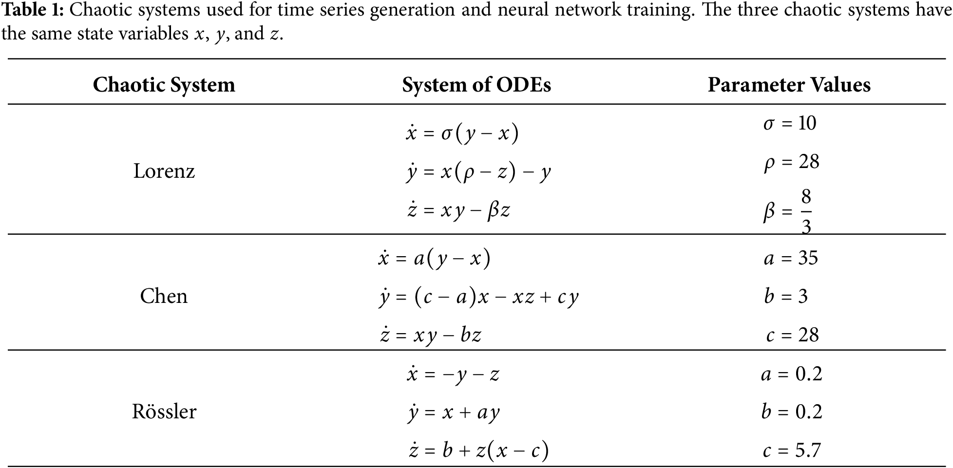
Fig. 1 shows the attractors corresponding to the (a) Lorenz, (b) Chen, and (c) Rössler systems, respectively. The time series are generated by numerically integrating each system using a step size of h=0.002 for the Lorenz system, h=0.0015 for the Chen system, and h=0.005 for the Rössler system. A uniform sampling process is then applied, for the case study of the proposed work, the sampling is performed to extract one sample every 20 integration steps for all systems. The samples per state variable that are saved result in 8000 samples for the Lorenz and Rössler systems, and 9500 samples for the Chen system. A sliding window of length 1 is employed to construct the input-output pairs used for training the proposed MLPs. For the three chaotic systems, the MLPs consist of two hidden layers with seven neurons each and a Rectified Linear Unit (ReLU) as the activation function. The training of the MLPs is carried out using the Limited-memory Broyden-Fletcher-Goldfarb-Shanno (L-BFGS) optimizer for the Lorenz and Rössler systems, and Adaptive Moment Estimation (ADAM) optimizer for the Chen system, with a maximum of 5000 iterations, a convergence tolerance of 10−4, and a random seed of 5. Both the input and output variables are normalized in the interval [−1,1] using MinMaxScaler normalization. The training process ends when either the convergence tolerance is achieved or the maximum number of iterations is reached. All simulations and training procedures have been implemented in Python 3.11.9 using NumPy, Scikit-learn, and Matplotlib.

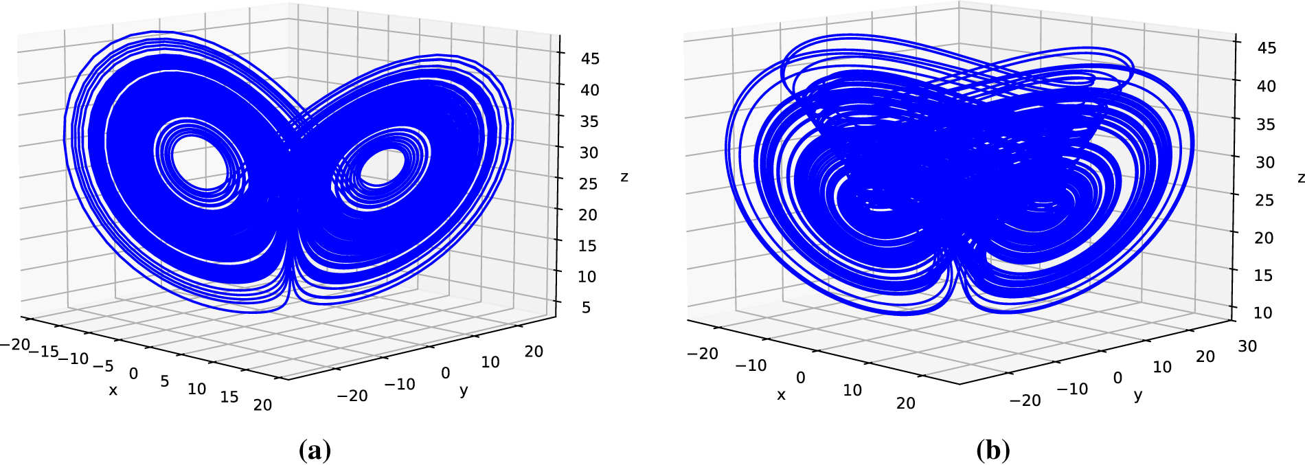
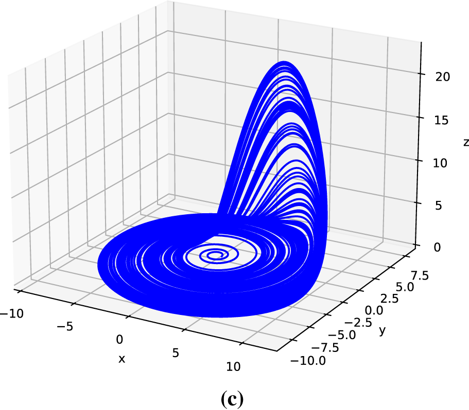
Figure 1: Chaotic attractors generated by numerically integrating each system: (a) Lorenz, (b) Chen, and (c) Rössler systems.

3  Multilayer Perceptron Training and Time Series Reconstruction

To model the dynamics of the chaotic systems, an MLP topology is generated using the scikit-learn library available in the Python environment [16]. The overall methodology, including data normalization, neural network training, accuracy evaluation, and iterative reconstruction, is summarized in Fig. 2.

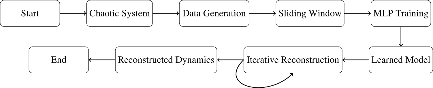
Figure 2: General framework for learning and reconstructing chaotic dynamics using an MLP-based regressor.

The MLP is trained using time series generated from the chaotic systems described in the previous section. The input dataset is constructed using a sliding window approach, where a sequence of past state values is used to reconstruct the next state of the system. This supervised learning approach allows the MLP to approximate the nonlinear mapping that governs the temporal evolution of the chaotic system.

3.1 Data Normalization

The chaotic time series are normalized to improve numerical stability during the training process and to facilitate subsequent hardware implementation. Normalization is performed using the MinMaxScaler method, which scales the data to a specified range. In the proposed work, both the input and output data are scaled in the interval [−1,1], according to

xnorm=2⋅x−xminxmax−xmin−1,(1)

where x is the original value, and xnorm is the normalized value. This normalization improves the convergence of the training algorithm, prevents saturation of activation functions, and facilitates FPGA implementation using fixed-point arithmetic representation, as shown in the following sections.

3.2 Architecture and Training of the Multilayer Perceptron

The implemented neural models correspond to fully connected MLPs composed of one input layer, two hidden layers, and one output layer. The number of neurons in the hidden layers is defined according to the chaotic system being modeled. The output layer consists of three neurons corresponding to the reconstructed state variables of the system. The general architecture of the proposed MLP is illustrated in Fig. 3.

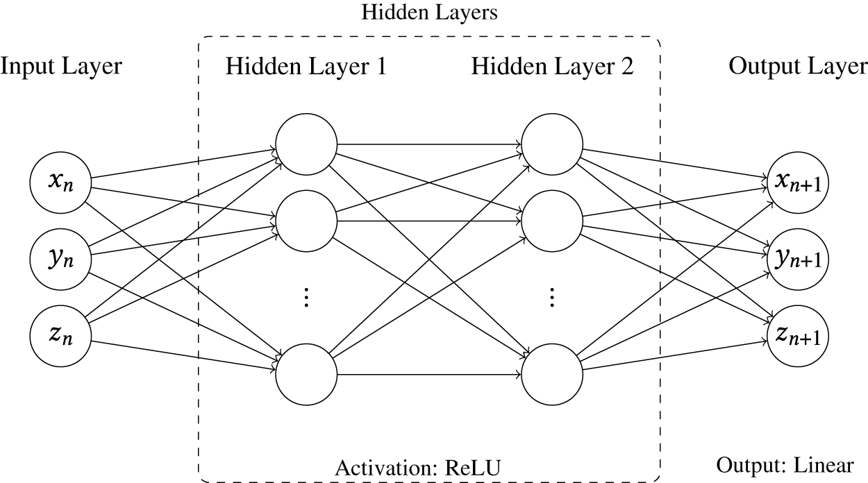
Figure 3: Architecture of the multilayer perceptron used for modeling chaotic dynamics.

The proposed MLPs are trained using the MLPRegressor function with the L-BFGS (Limited-memory Broyden-Fletcher-Goldfarb-Shanno) quasi-Newton optimization algorithm and the Adam (Adaptive Moment Estimation) optimization algorithm. L-BFGS is well suited for regression problems with moderate-sized datasets and provides fast convergence and high accuracy, while Adam offers efficient stochastic optimization with adaptive learning rates, making it suitable for training neural networks with large and complex datasets.

The activation function used in the hidden layers depends on the chaotic system. The Rectified Linear Unit (ReLU) activation function is used for all three chaotic systems. These nonlinear activation functions enable the MLPs to approximate the nonlinear dynamics of the chaotic systems.

Table 2 summarizes the architecture and training parameters of the proposed MLP models used to learn the dynamics of the Lorenz, Chen, and Rössler chaotic systems. The network receives a vector composed of past state values as input and reconstructs the next state of the system, enabling time series reconstruction.

During training, the synaptic weights and bias parameters are iteratively adjusted to minimize the error between the reconstructed outputs and the target values. After training is completed, the neural network parameters, including weight matrices and bias vectors, are extracted and used for hardware implementation in the FPGA.

3.3 Neural Model Accuracy

The accuracy of the neural network models is evaluated using two widely adopted regression performance metrics: the Mean Squared Error (MSE) and the coefficient of determination (R2).

The Mean Squared Error is defined by Eq. (2),

MSE=1N∑i=1N(yi−y^i)2,(2)

and the coefficient of determination is defined by Eq. (3),

R2=1−∑i=1N(yi−y^i)2∑i=1N(yi−y¯)2,(3)

where yi represents the true value, y^i represents the reconstructed value, y¯ represents the mean value of the dataset, and N is the total number of samples.

The MSE measures the average squared reconstruction error, while the R2 coefficient quantifies the proportion of variance explained by the model. Values of R2 close to 1 indicate high reconstruction accuracy.

Table 3 summarizes the accuracy metrics obtained after training the proposed MLP models for each chaotic system. The results demonstrate that the neural networks achieve high reconstruction accuracy and are capable of learning the nonlinear dynamics of the chaotic systems.

3.4 Reconstruction of Chaotic Trajectories

After training, the MLP is used to iteratively reconstruct the temporal evolution of the chaotic systems. The reconstruction process begins with an initial input vector composed of previously observed samples. The neural network generates the next reconstructed state, which is then fed back as input to reconstruct subsequent states.

This iterative process can be expressed by Eq. (4),

x^(n+1)=f(x^(n),x^(n−1),...,x^(n−k)),(4)

where f(⋅) represents the nonlinear function learned by the multilayer perceptron. This approach enables the MLP to reconstruct the system trajectory without requiring explicit knowledge of the governing ODEs.

The reconstructed trajectories allow visualization of the chaotic attractors in phase space. Fig. 4 shows the reconstructed trajectory for the Lorenz system, while Figs. 5 and 6 show the reconstructed trajectories for the Chen and Rössler systems, respectively.

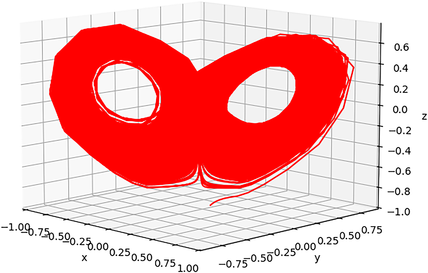
Figure 4: Reconstructed trajectory by the MLP for the Lorenz system.

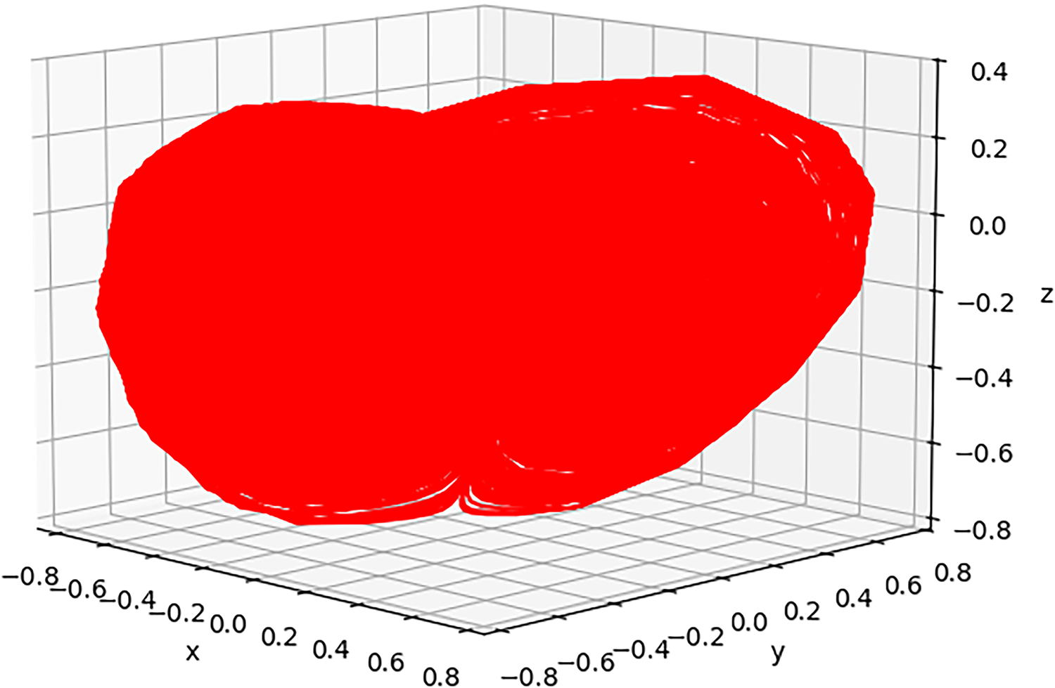
Figure 5: Reconstructed trajectory by the MLP for the Chen system.

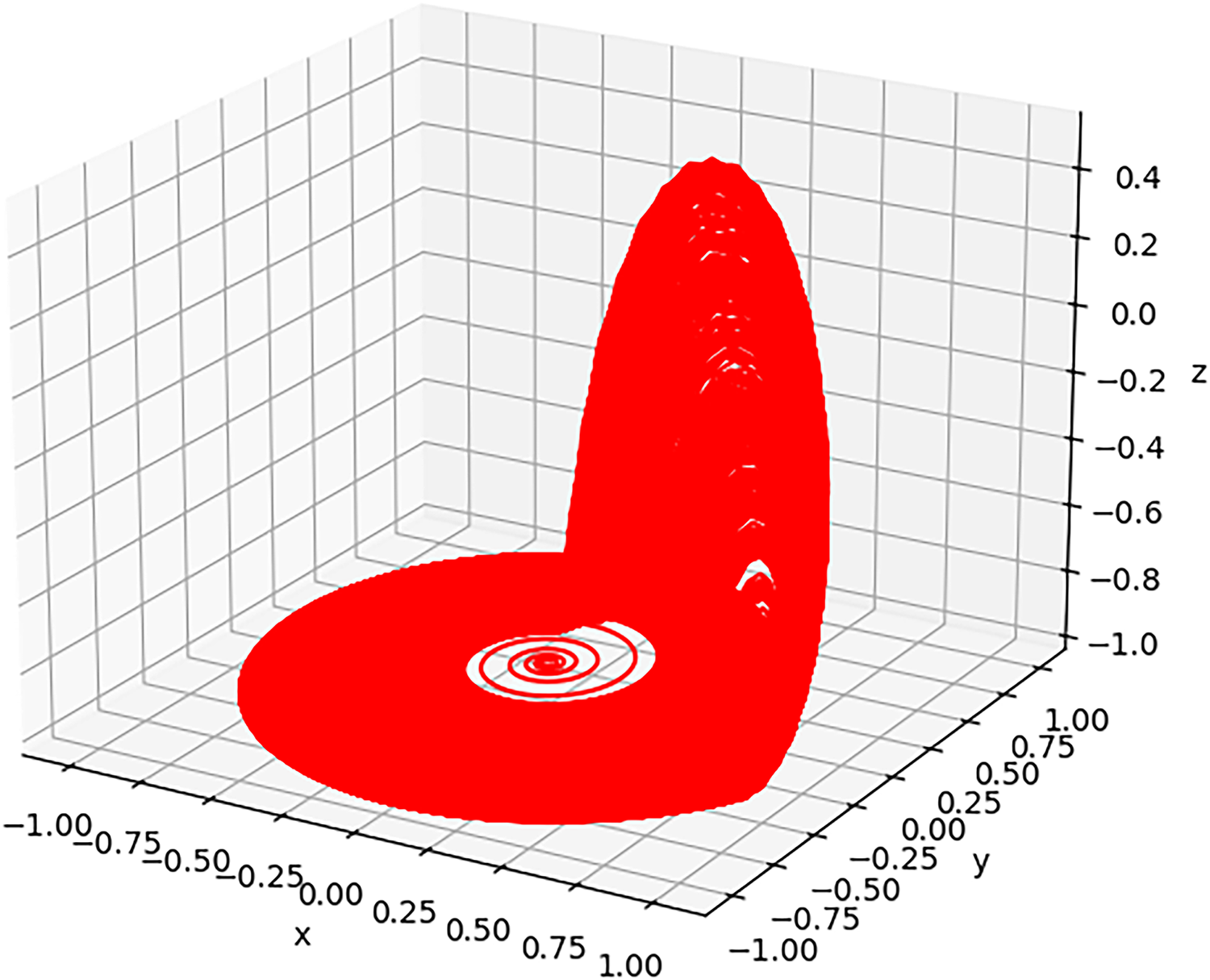
Figure 6: Reconstructed trajectory by the MLP for the Rössler system.

The results demonstrate that the proposed MLPs successfully reproduce the characteristic structure of the chaotic attractors and preserve their nonlinear dynamical behavior. Furthermore, the extracted synaptic weights and bias parameters can be directly implemented in hardware, enabling real-time reconstruction of chaotic systems using FPGA devices.

4  Python Verification of the MLPs

In order to validate the correct operation of the trained neural network models, a verification stage was performed with Python scripts. This step allows confirming that the parameters obtained during the training process, namely the synaptic weight matrices and bias vectors, are capable of accurately reconstructing the dynamics of the chaotic systems studied, regardless of the original training platform.

For each chaotic system, a fully connected MLP is implemented using the previously extracted parameters. The reconstruction process is carried out through forward propagation, where the output of each layer is computed as the weighted sum of its inputs plus a bias term, followed by a nonlinear activation function. Rectified Linear Unit (ReLU) activation function has been used, which is defined by Eq. (5),

ReLU(x)=max(0,x).(5)

The forward propagation through the MLP can be expressed in a general form by Eq. (6),

mlp(x)=f(f(x⋅W1+b1)⋅W2+b2)⋅W3+b3,(6)

where:

•   x and bi, for i={1,2,3}, are row vectors.

•   Wi, for i={1,2,3}, are weight matrices.

•   f(⋅) denotes the ReLU activation function.

•   x is the input state vector (three-dimensional for all the three studied systems).

•   W1 and b1 are the weight matrix and bias vector of the first hidden layer.

•   W2 and b2 are the weight matrix and bias vector of the second hidden layer.

•   W3 and b3 are the weight matrix and bias vector of the output layer.

•   mlp(x) is the reconstructed output representing the next state of the chaotic system.

The activation functions introduce the nonlinearity required for the neural network to approximate the highly nonlinear behavior of chaotic systems. Regarding the Python code of the MLP for modeling chaotic systems: The matrices and bias vectors must be initialized with the numpy.array function, and then the evaluation of the neural network, for any of the three chaotic systems, could be described as

def eval ( x ) :

    o1 = x @ W1 + b1

    o1 = np.where( o1 > 0, o1, 0 )  # The ReLU function

    o2 = o1 @ W2 + b2

    o2 = np.where( o2 > 0, o2, 0 )

    o3 = o2 @ W3 + b3

    return o3

After implementing the neural network models in Python, the reconstructed trajectories of each chaotic system are generated. Fig. 7 shows the reconstructed Lorenz attractor using 30,000 points generated by the MLP, clearly preserving its characteristic double-scroll structure. Similarly, Fig. 8 presents the reconstructed Chen attractor using 30,000 points. Finally, Fig. 9 shows the reconstructed Rössler attractor using 30,000 points to represent its dynamical behavior.

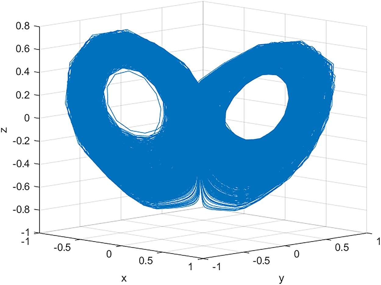
Figure 7: Reconstructed Lorenz attractor using the trained neural network model.

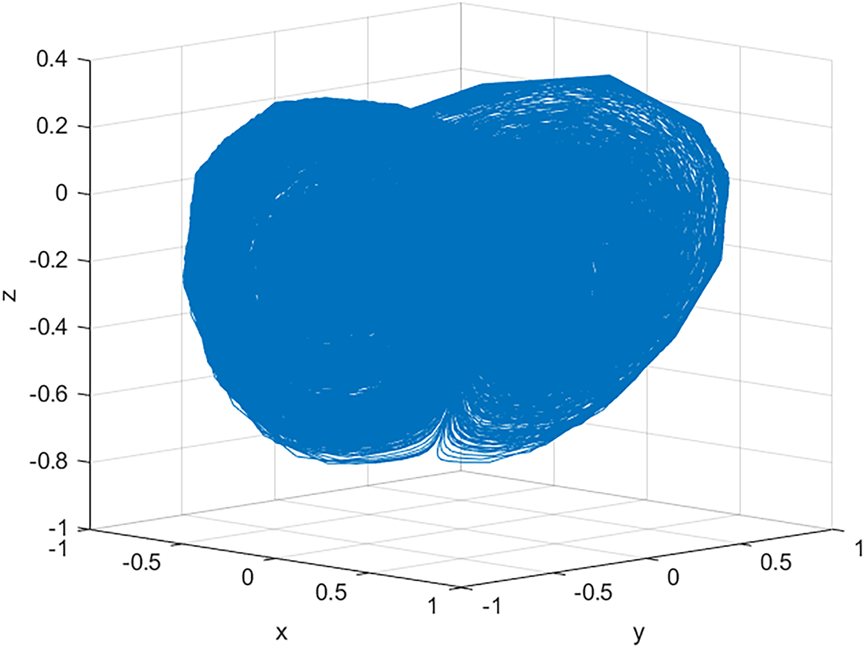
Figure 8: Reconstructed Chen attractor using the trained neural network model.

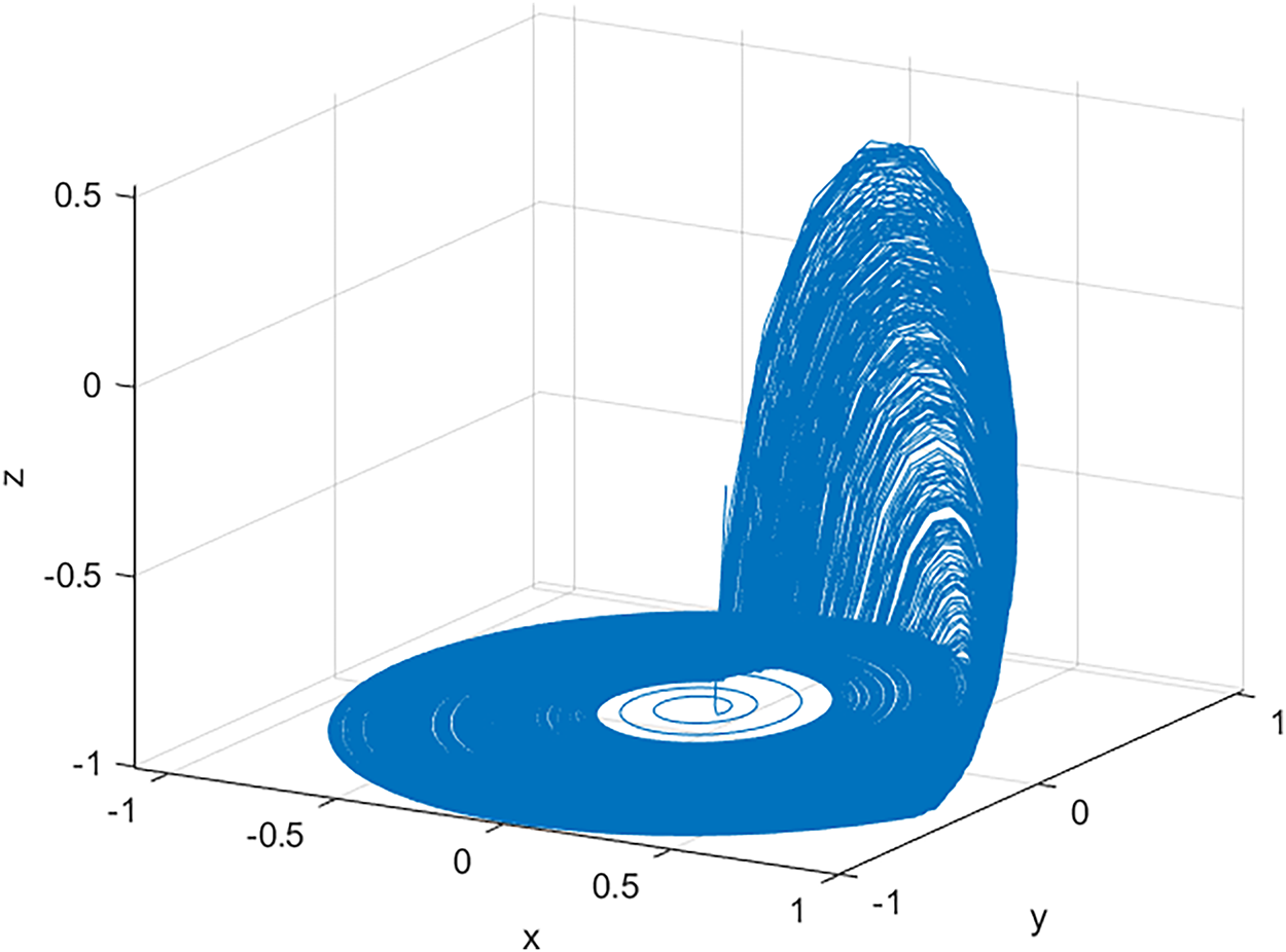
Figure 9: Reconstructed Rössler attractor using the trained neural network model.

The obtained results demonstrate that the reconstructed trajectories preserve the essential geometric and dynamical properties of the original attractors, including their shape, orientation, and phase-space evolution. These results confirm that the trained neural network models are capable of accurately approximating the underlying nonlinear dynamics of the chaotic systems. Furthermore, this verification stage validates the correctness of the extracted parameters and confirms their suitability for hardware implementation in FPGA-based architectures.

5  FPGA Implementation of the MLPs Generating Chaotic Time Series

In Eq. (6), one can identify arithmetic operations that can be associated to digital blocks, which can be implemented in an FPGA with Verilog Hardware description. The digital blocks that can be seen are, for example, adders, matrix multipliers, PIPO registers, control unit, ROM/RAM memories, and the ReLU function. A ReLU block implements the activation function of neural networks that outputs the input directly if it is positive or zero, and zero if it is negative. Fig. 10 shows the block diagram description of Eq. (6) that is used for the reconstruction of Lorenz chaotic system. It is worth mentioning that the Matrix multiplier is typically evaluated by computing C=A×B, where each element Cij is the dot product of row i from matrix A and column j from matrix B, and ROM/RAM memories are implemented with logic resources and Look-up tables (LUTs) [17].

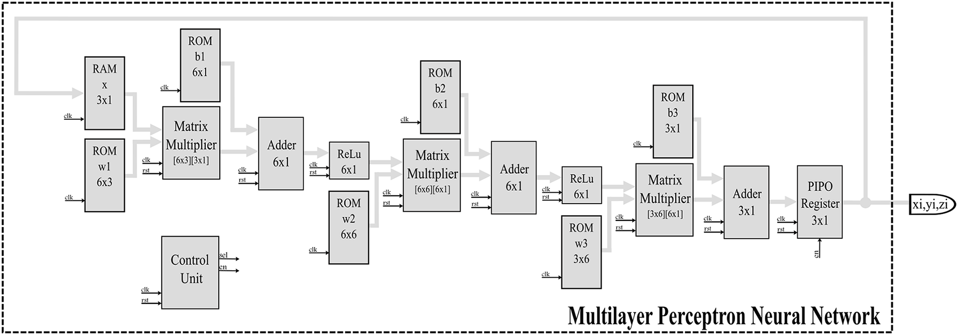
Figure 10: Block description of the MLP for Lorenz system.

For the MLP modeling Lorenz system, the values obtained for the three weight matrices and three bias vectors corresponding to Eq. (6), are:

W1=[7.41504315e−013.09220200e−01−1.32235205e−016.83367382e−011.07094561e−018.42985027e−021.38631933e−01−2.71431895e−01−2.59093351e−01−5.09783961e−01−8.22078086e−016.68356230e−015.39370761e−01−1.93621310e−017.75076142e−01−3.68795796e−01−8.35452532e−01−2.49683782e−04]b1=[0.98878053−0.812450620.84720894−0.382415780.66093551−0.13311896]

W2=[−0.590417680.269452440.066308540.940899660.01575165−0.22322202−0.69440962−0.16720287−0.091673420.39136034−0.56372340.10979630.41011643−0.631387890.997781270.30015407−0.553979680.650025850.523772540.59766463−0.70374744−0.043135990.68067912−0.142867350.820606360.478265051.219296530.46615663−0.482061810.08431699−0.282505010.11415532−0.10837661−0.074263580.989679010.12957186]b2=[−0.148174160.974323390.63132653−0.385938910.90889249−0.55032309]

W3=[−0.11142006−0.460409060.040919030.575104610.43329095−1.18143307−0.58478348−0.597348840.567661420.6721905−0.279572840.47521759−0.004780970.070560821.243302410.231970431.085862250.02596217]b3=[0.068994451.34956254−0.92933618]

Similarly, Figs. 11 and 12 show the implementation of the corresponding MLPs for the reconstruction of Chen and Rössler chaotic oscillators that use ReLU activation function.

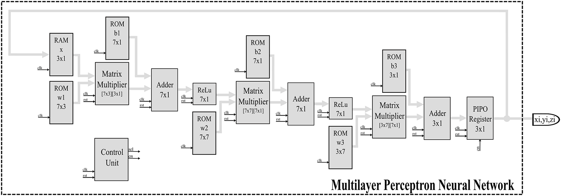
Figure 11: Block description of the MLP for Chen system.

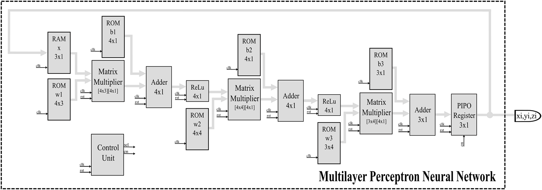
Figure 12: Block description of the MLP for Rössler system.

For the MLP modeling Chen system, the values obtained for the three weight matrices and three bias vectors corresponding to Eq. (6), are:

W1=[−0.649733200.53986956−0.55193782−4.4262590e−043.3480637e−343.3700332e−110.35750274−0.29941512−0.32752226−0.70274384−6.8743138e−013.4594185e−05−5.9294892e−21−0.878209940.41710675−0.32503704−0.38482740−3.9268034e−019.0323116e−102.8049948e−150.33509090]b1=[0.14196793−0.3548878−0.12557340.47165751−0.5512583−0.518030330.76066832]

W2=[4.21291430e−01−3.43352257e−01−8.75254091e−01−3.14953989e−01−1.32846824e−016.17155993e−01−2.59182016e−012.38684161e−18−8.39670047e−038.18226019e−037.12429391e−026.99166872e−03−2.57231642e−012.38834906e−025.76396087e−01−9.84803726e−02−7.61452793e−01−1.68528647e−013.83533860e−011.28949791e−016.26947766e−019.41313021e−023.97819660e−01−5.71862646e−01−5.50302330e−01−5.12729389e−01−7.92556017e−013.58927530e−015.07394263e−033.09966801e−111.39521559e−04−1.06738559e−215.94954208e−111.17273527e−042.57399767e−031.93985421e−031.85644863e−04−1.67827528e−03−1.10950727e−10−5.03912396e−03−1.53171799e−276.33681893e−05−2.85621773e−01−3.66564465e−01−2.63568320e−01−3.68318074e−019.44150826e−01−1.24291339e−023.72539418e−01]b2=[−0.2443870.343576070.494737150.61069155−0.069887950.70672109−0.14113199]

W3=[0.184621670.265498510.440291790.471797000.40404557−0.530888620.55505058−0.345092340.077033100.580538290.311516950.319425470.01121729−1.158604990.89651608−0.141656721.121727860.54056582−1.02606559−0.53977168−0.36374211]b3=[0.239921490.06022083−0.50313945]

Finally, for the MLP modeling Rössler system, the values obtained for the three weight matrices and three bias vectors corresponding to Eq. (6), are:

W1=[−0.784666830.46605654−0.376089630.82700084−0.404165370.291958390.787839000.287139430.05111379−0.263395570.045130910.97924925]b1=[0.88374683−0.978677151.046680460.39348465]

W2=[−0.10650373−1.001849090.22306381−0.22372422−0.03260540−0.33340427−0.37292933−0.398049280.023607650.56905731−0.579166710.915806851.15950765−0.29299479−0.82391268−0.44698748]b2=[0.020395881.2836078−0.826304120.39582269]

W3=[−0.279500150.397496090.918529151.303433580.426924590.024845490.685990950.78276828−0.92170617−1.480996120.79926418−0.01621099]b3=[0.354305−1.32626345−0.99627959]

In an FPGA, the blocks can be designed by adopting fixed-point representation. As the data is normalized in the range [−1, 1], the computer arithmetic can be established to have the format 1.1.30 (32 bits), i.e., using one bit to represent the sign, 1 for the integer part, and 30 for the fractional part. This format depends on the multiplication blocks of the FPGA implementation, which can be observed by performing numerical simulations.

Table 4 shows the hardware resources for the FPGA implementation of Eq. (6) by using the Cyclone IV EP4CGX150DF31C7 device of the DE2i-150 board using the Quartus II 18.1 synthesizer. The row called “Clock cycles by iteration” represents the number of clock cycles that are required to process a new iteration to compute mlp(x) with valid data, and the “Latency” row represents the time to compute a new iteration with a 50 MHz clock signal. Fig. 13 shows the experimental setup to implement the proposed MLP model for Lorenz system reconstruction on the DE2i-150 board. In addition, a 16-bit Digital-to-Analog Converter (DAC) is used to visualize the results in a Teledyne oscilloscope. Fig. 14 shows the experimental Lorenz chaotic time series generated from the FPGA implementation. Fig. 15 shows the experimental Lorenz chaotic attractor from the FPGA implementation of the MLP for reconstruction.

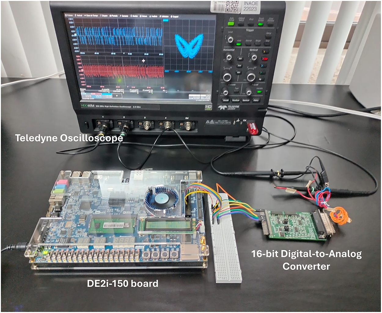
Figure 13: Experimental setup to implement the Lorenz Chaotic system reconstructed, using a Cyclone IV EP4CGX150DF31C7 device of DE2i-150 board, a 16-bit Digital-to-Analog Converter and a Teledyne Lecroy oscilloscope to visualize the attractor.

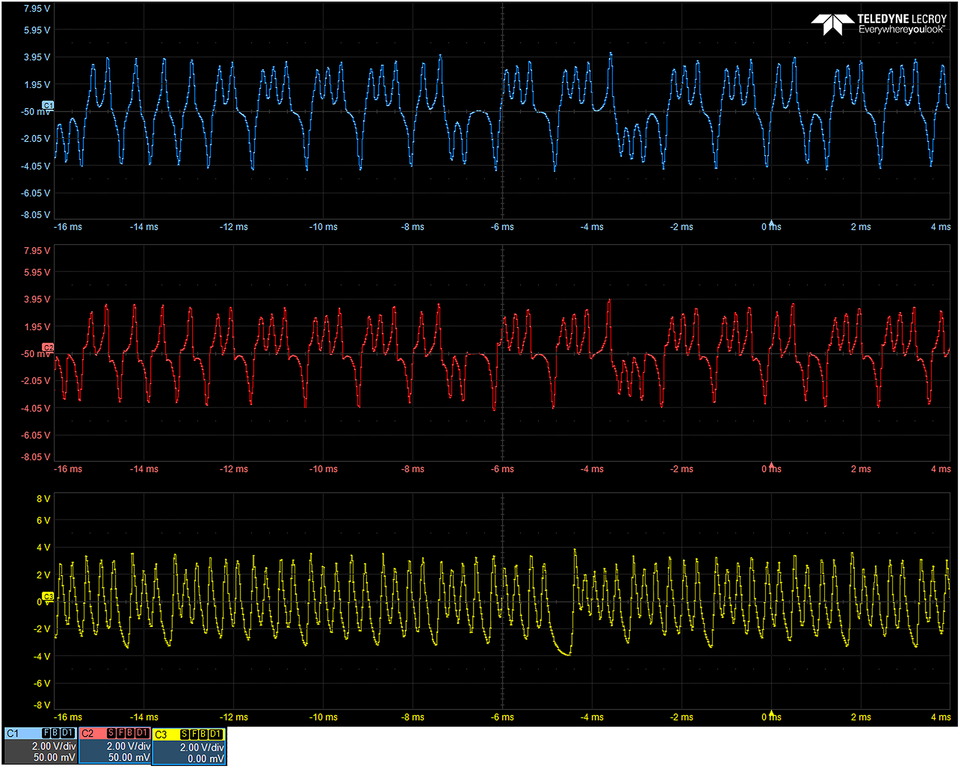
Figure 14: Experimental time series of Lorenz Chaotic system reconstructed and observed in an oscilloscope.

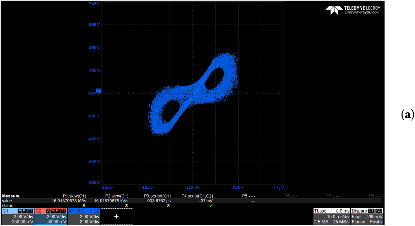
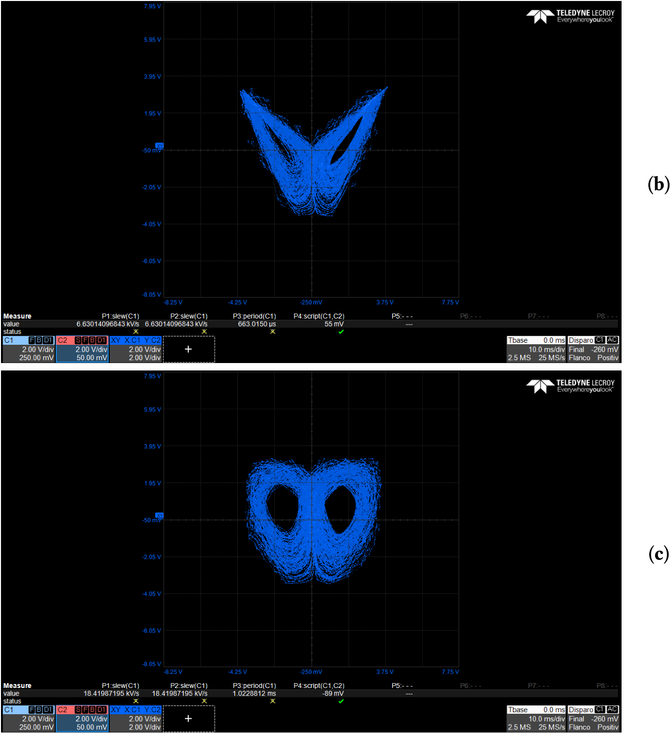
Figure 15: Experimental attractors of Lorenz Chaotic system reconstructed and observed in an oscilloscope. (a) x-y view, (b) x-z view, and (c) y-z view.

Similarly, the Chen and Rössler chaotic systems are reconstructed and their experimental time series are shown in Figs. 16 and 17, respectively. Finally, the experimental attractors are shown in Figs. 18 and 19.

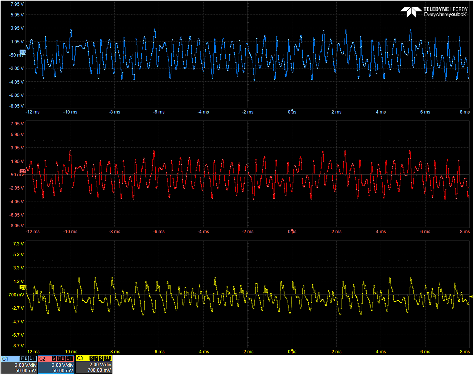
Figure 16: Experimental time series of Chen Chaotic system reconstructed and observed in an oscilloscope.

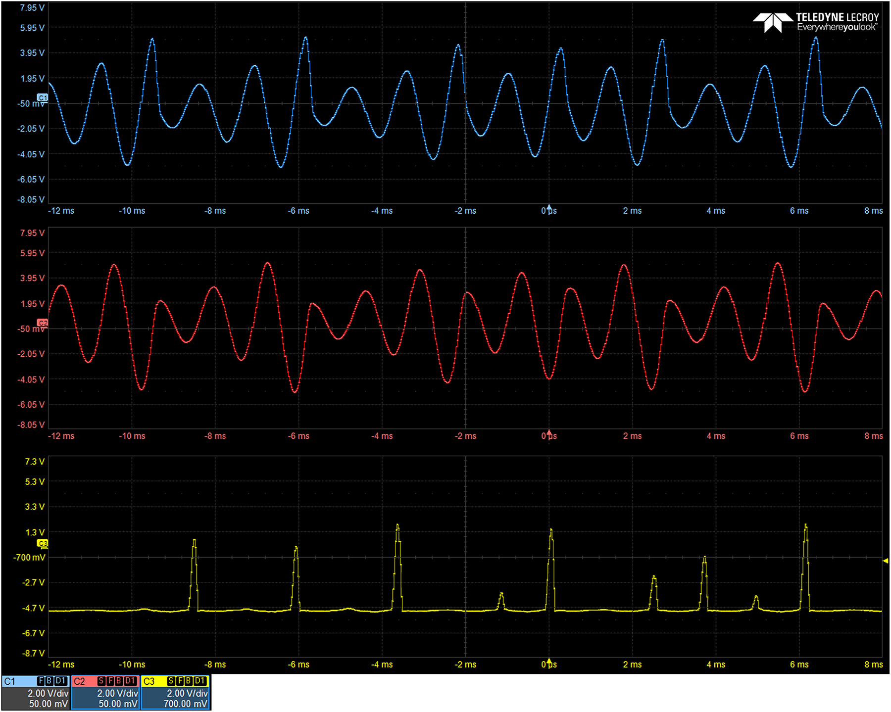
Figure 17: Experimental time series of Rössler Chaotic system reconstructed and observed in an oscilloscope.

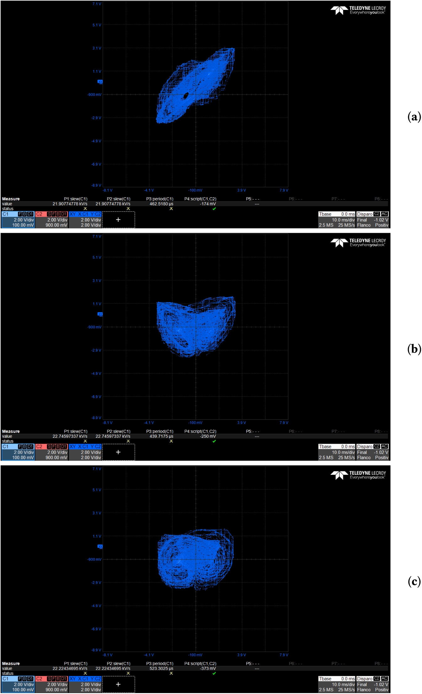
Figure 18: Experimental attractors of Chen Chaotic system reconstructed and observed in an oscilloscope. (a) x-y view, (b) x-z view, and (c) y-z view.

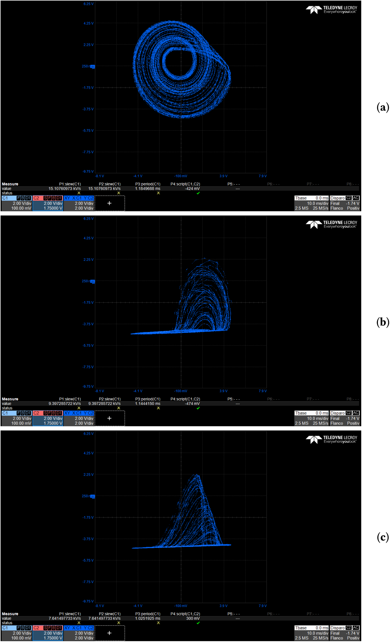
Figure 19: Experimental attractors of Rössler Chaotic system reconstructed and observed in an oscilloscope. (a) x-y view, (b) x-z view, and (c) y-z view.

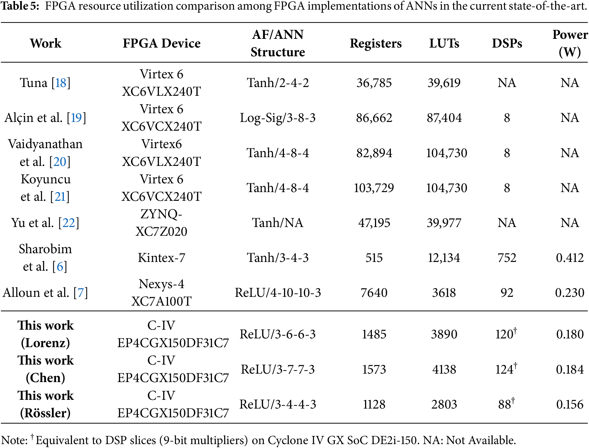
Table 5 presents a quantitative comparison of FPGA resource utilization between the proposed MLP implementations and recent state-of-the-art works. As one can see, the Lorenz, Chen, and Rössler hardware implementations require between 1128–1573 slice registers, 2803–4138 slice LUTs, and between 88–124 digital signal processors (DSPs), with a thermal power consumption ranging from 0.156 to 0.184 W. These results are presented alongside existing implementations for reference and comparison purposes.

6  Pseudo Random Number Generators from MLPs Data

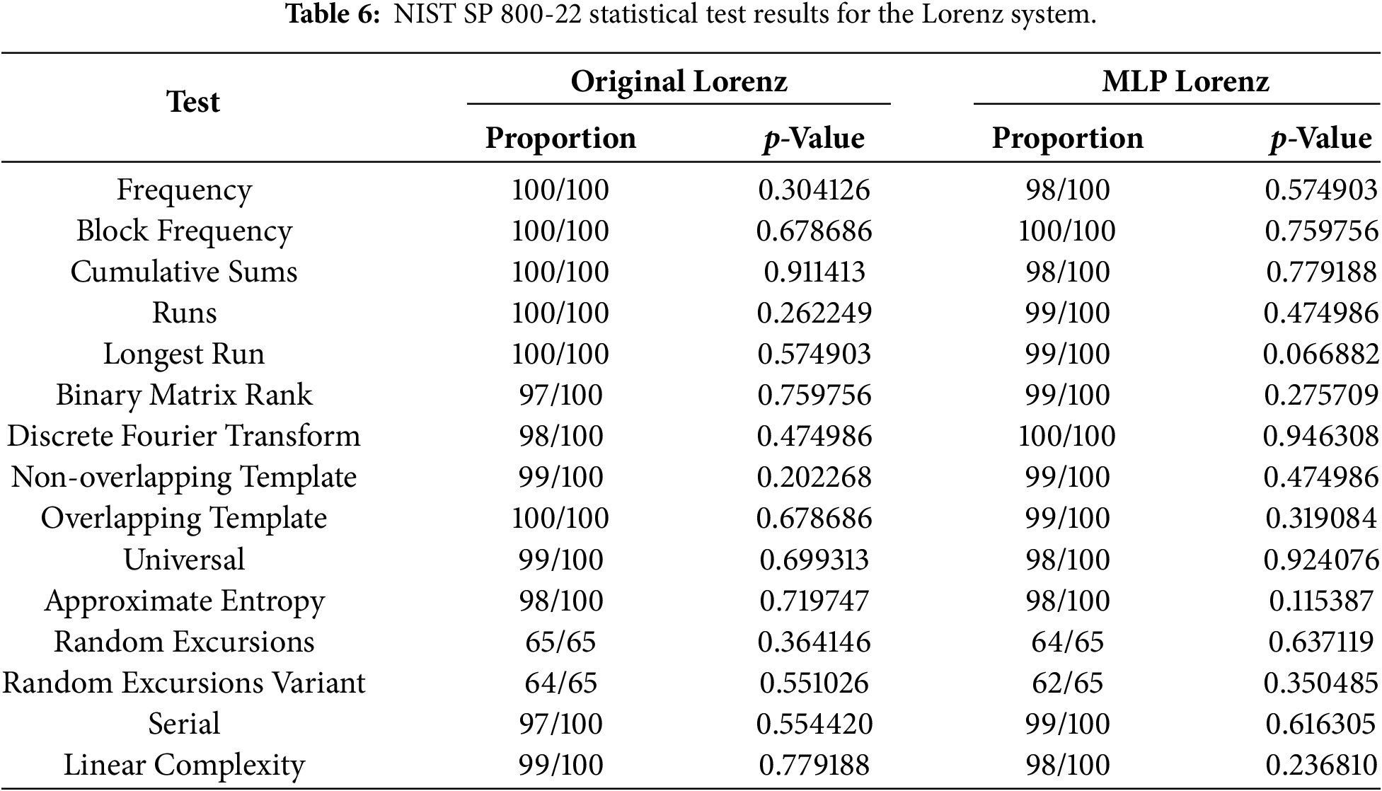
With the data generated by the three MLPs that model each chaotic system, namely: Lorenz, Chen, and Rössler, three pseudo-random number generators (PRNGs) have been constructed.

Here, the MLPs have been programmed in Python, which uses, by default, floating-point numbers with double precision. The proposed work has been performed by using the procedure described in [23], which is developed by using the Python function frexp to convert a floating-point number into normalized fractional and integral components. The integral component is the exponent, and it is an integer number. The fractional component is a floating point number and is always in the range [0.5,1). Then, this fractional component is multiplied by 240 = 1,099,511,627,776 and the eight least significant 25 bits are taken as the pseudo-random bits. Thus, as the chaotic system is three-dimensional, 24 pseudo-random bits are generated in each iteration, and the generated bits are concatenated to form a sequence of pseudo-random bits.

For each time series, a sequence of 100×106 bits was generated and analyzed with the TestU01 and NIST statistical test. The former test applies Rabbit, Alphabit, and Block Alphabit, which consist in 40, 17, and 240 tests, respectively. In the proposed work, all TestU01 tests passed for all the three PRNGs. Tables 6–8 present the NIST SP 800-22 statistical test results for the Lorenz, Chen, and Rössler chaotic systems, respectively. For each system, both the original and reconstructed (MLP) sequences are evaluated. The tables report the proportion of sequences that passed each test and the corresponding p-values. The results demonstrate that all three chaotic systems produce high-quality pseudo-random sequences, with pass rates consistently above the NIST minimum requirements, validating their potential for use in security-oriented applications.

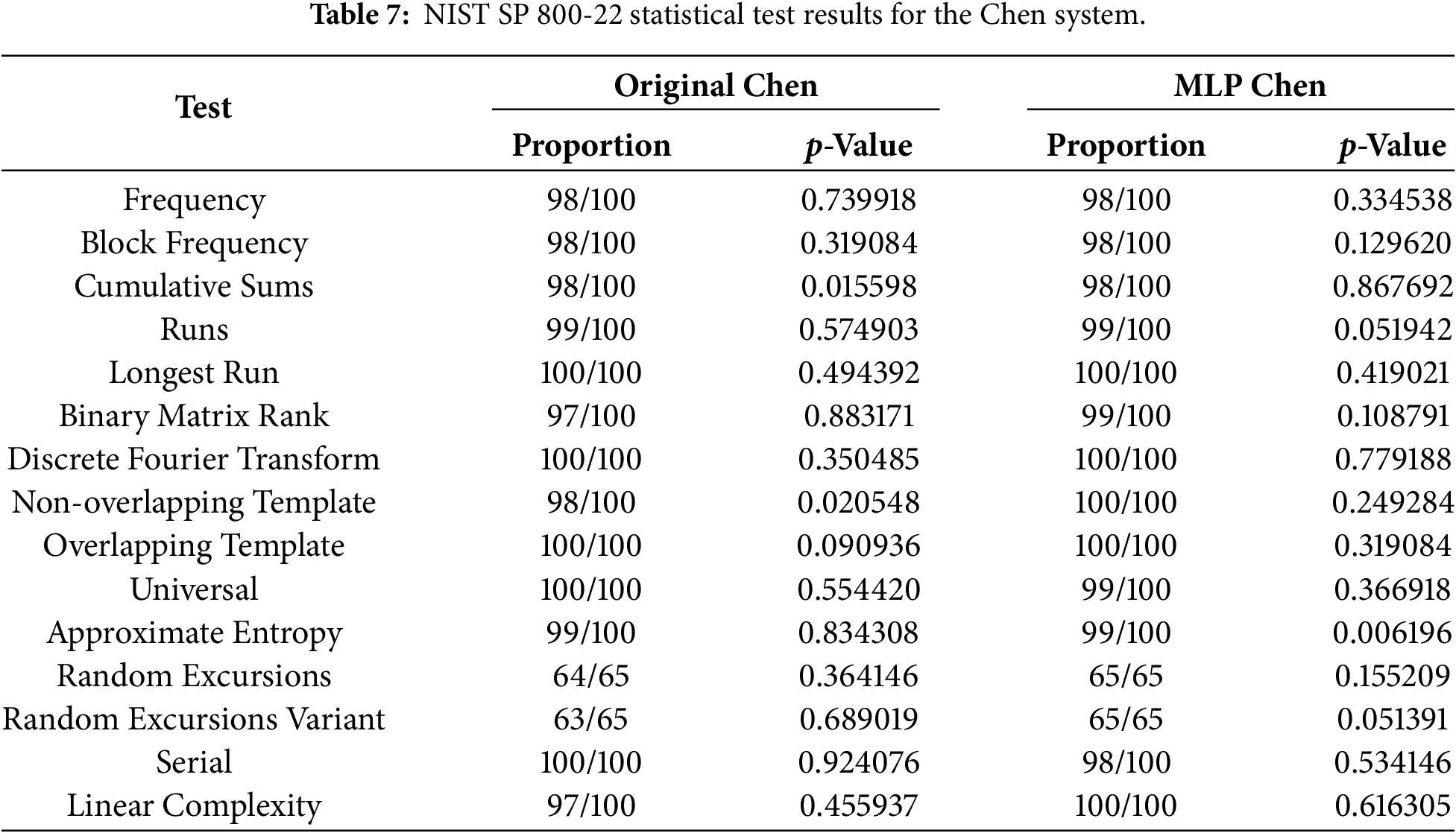
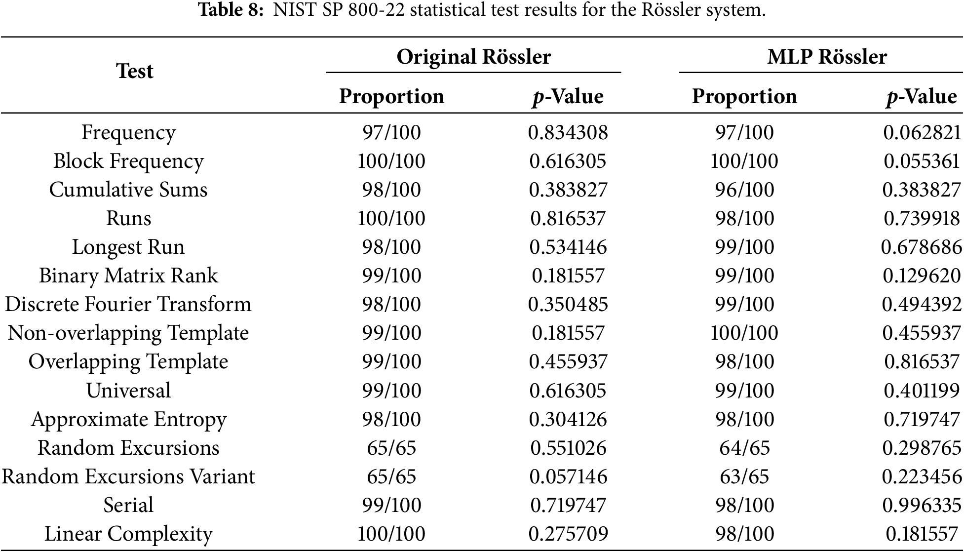
To demonstrate an advantage of using an MLP—such as those proposed for each chaotic system—instead of the three equations of each chaotic system, the domain of attraction was calculated for all the systems and all the MLPs. There were no differences in the case of the Lorenz and Rössler systems. For the Chen system, the calculated domain of attraction is shown in Fig. 20. As it is possible to see in this figure, for the associated MLP, one can use all the possible initial values in x and y in the searched space; this also means that the key space could be bigger for the PRNG constructed with the respective MLP model.

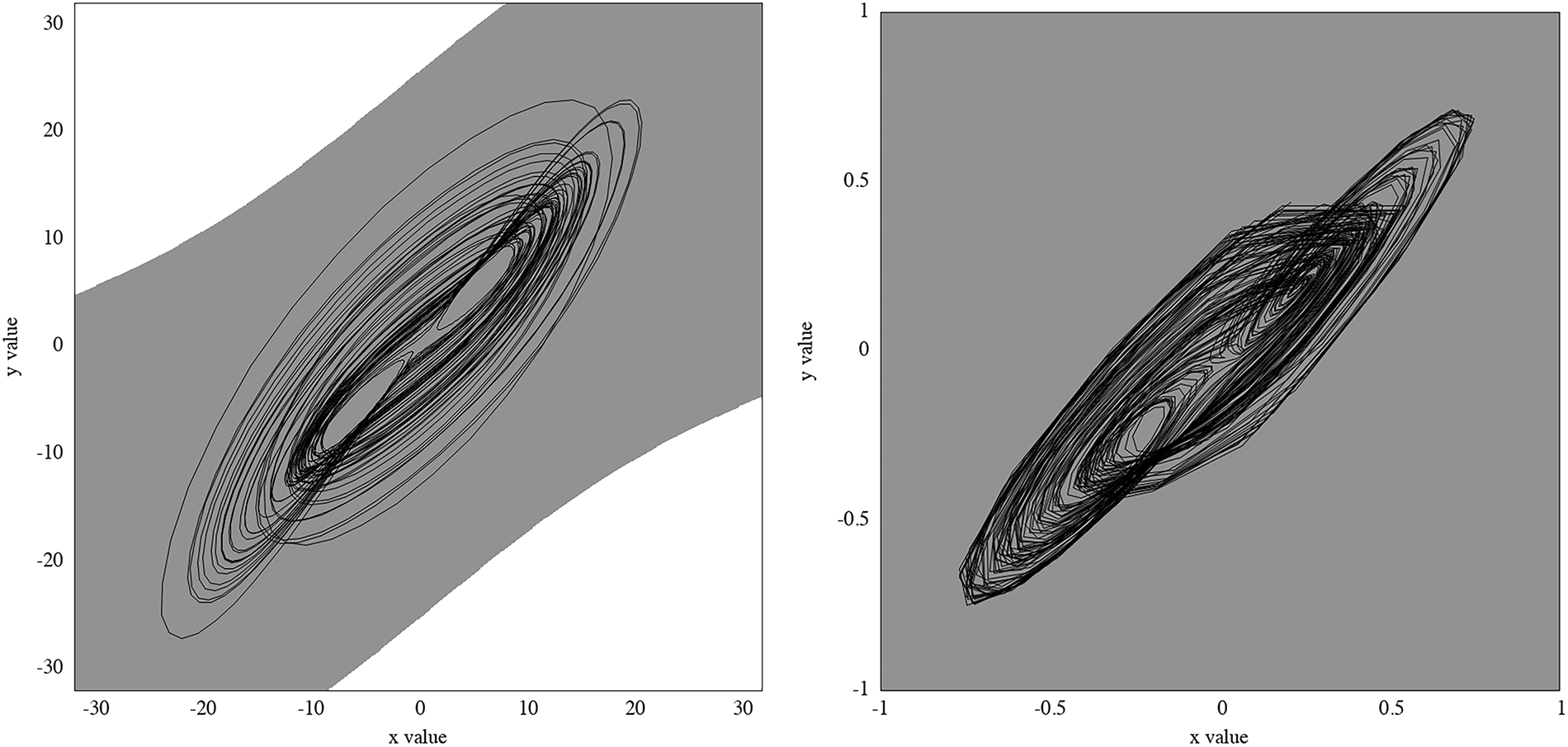
Figure 20: Domains of attraction for the Chen oscillator, at the left, and for its respective neural network, at the right.

7  Conclusion

It has been shown that chaotic attractors can be generated from the artificial neural network of a mathematical model describing a chaotic system. Throughout the manuscript, the generation of an MLP model for the Lorenz, Chen, and Rössler chaotic systems has been detailed. The trained MLPs were implemented on an FPGA using Verilog-HDL. The MLP models for each chaotic system were validated in Python and synthesized on an FPGA through the reconstruction of Lorenz, Chen, and Rössler time series.

From the weight matrices given in Section 5, it can be appreciated that they are too small compared to the state of the art. The largest one is of size W2 = 7 × 7 for the MLP modeling the Chen system, and the others are small to generate MLPs with a reduced number of neurons.

For the design of a PRNG, the eight least significant bits were taken for each data point from each state variable of the chaotic systems. As the systems are 3D, 24 pseudo-random bits are generated in each iteration, which were concatenated to form a sequence of pseudo-random bits. In this manner, for each time series, a sequence of 100×106 bits was generated and analyzed with the TestU01 and NIST statistical tests, and all of them passed.

To show the advantage of using an MLP model, as the proposed ones for each chaotic system, instead of the ODEs, the domain of attraction was calculated for all the systems and all the MLPs. For the Lorenz and Rössler systems, there were no differences. However, for the Chen system, the calculated domain of attraction is shown in Fig. 20. This indicates that it is possible to use all possible initial values in x and y in the searched space, leading to state that the key space could be bigger for the PRNG constructed with the respective MLP model.

With real chaotic signals, one limitation can be associated to the sampling problem, which consists of getting enough samples to train the neural network. The critical point here is that depending on the set of samples (data), the domain of attraction can be very small and not continuous.

Finally, the FPGA implementations of the MLP models demonstrate their feasibility and efficiency for nonlinear dynamical system modeling and real-time series prediction.

Acknowledgement: None.

Funding Statement: The authors received no specific funding for this study.

Author Contributions: The authors confirm contribution to the paper as follows: Conceptualization, Omar Guillén-Fernández, Carlos Alejandro Velázquez-Morales, Luis Gerardo de la Fraga, Sajad Jafari and Esteban Tlelo-Cuautle; methodology, Omar Guillén-Fernández, Carlos Alejandro Velázquez-Morales, Luis Gerardo de la Fraga, Sajad Jafari and Esteban Tlelo-Cuautle; software, Omar Guillén-Fernández and Carlos Alejandro Velázquez-Morales; validation, Omar Guillén-Fernández, Carlos Alejandro Velázquez-Morales, Luis Gerardo de la Fraga and Esteban Tlelo-Cuautle; formal analysis, Omar Guillén-Fernández, Carlos Alejandro Velázquez-Morales and Luis Gerardo de la Fraga; investigation, Omar Guillén-Fernández, Carlos Alejandro Velázquez-Morales and Luis Gerardo de la Fraga; resources, Omar Guillén-Fernández, Carlos Alejandro Velázquez-Morales and Luis Gerardo de la Fraga; data curation, Omar Guillén-Fernández, Carlos Alejandro Velázquez-Morales and Luis Gerardo de la Fraga; writing—original draft preparation, Omar Guillén-Fernández, Carlos Alejandro Velázquez-Morales, Luis Gerardo de la Fraga and Sajad Jafari; writing—review and editing, Omar Guillén-Fernández, Carlos Alejandro Velázquez-Morales, Luis Gerardo de la Fraga and Esteban Tlelo-Cuautle; visualization, Omar Guillén-Fernández, Carlos Alejandro Velázquez-Morales, Luis Gerardo de la Fraga and Esteban Tlelo-Cuautle; supervision, Luis Gerardo de la Fraga and Esteban Tlelo-Cuautle; project administration, Luis Gerardo de la Fraga and Esteban Tlelo-Cuautle. All authors reviewed and approved the final version of the manuscript.

Availability of Data and Materials: The authors confirm that the data supporting the findings of this study are available within the article.

Ethics Approval: Not applicable.

Conflicts of Interest: Given their roles as the Guest Editors of this Special Issue, Esteban Tlelo-Cuautle and Luis Gerardo de la Fraga had no involvement in the peer review of this article and had no access to information regarding its peer review. Full responsibility for the editorial process for this article was delegated to another journal editor. The authors declare no other conflicts of interest.

References

1. Lorenz EN. Deterministic nonperiodic flow. J Atmos Sci. 1963;20(2):130–41. doi:10.1175/1520-0469(1963)020<0130:dnf>2.0.co;2. [Google Scholar] [CrossRef]

2. Chen G, Ueta T. Yet another chaotic attractor. Int J Bifurc Chaos. 1999;9(7):1465–6. doi:10.1142/s0218127499001024. [Google Scholar] [CrossRef]

3. Rössler OE. An equation for continuous chaos. Phys Lett A. 1976;57(5):397–8. doi:10.1016/0375-9601(76)90101-8. [Google Scholar] [CrossRef]

4. Liu Z. Chaotic time series analysis. Math Probl Eng. 2010;2010(1):720190. doi:10.1155/2010/720190. [Google Scholar] [CrossRef]

5. Liu X, Ren J. Image encryption via deep learning-based chaotic system reconstruction. J Inf Secur Appl. 2026;101(9):104545. doi:10.1016/j.jisa.2026.104545. [Google Scholar] [CrossRef]

6. Sharobim BK, Yacoub MH, Sayed WS, Radwan AG, Said LA. Artificial neural network Chaotic PRNG and simple encryption on FPGA. Eng Appl Artif Intell. 2023;126(1):106888. doi:10.1016/j.engappai.2023.106888. [Google Scholar] [CrossRef]

7. Alloun Y, Kifouche A, Azzaz MS, Madani M, Bourennane EB, Sadoudi S. Design and FPGA implementation of a novel cryptographic secure pseudo random number generator based on artificial neural networks and chaotic systems. Integration. 2025;103(140):102388. doi:10.1016/j.vlsi.2025.102388. [Google Scholar] [CrossRef]

8. Carvajal C, Manríquez R. Fractional fuzzy transform: integrating fuzzy approximation and fractional calculus. Appl Soft Comput. 2026;189(3):114483. doi:10.1016/j.asoc.2025.114483. [Google Scholar] [CrossRef]

9. Wang D, Lei Y, Shi P, Bian H, Luo C, Zhao J. Chaotic laser time series prediction based on an improved logistic mapping algorithm echo state network. Appl Opt. 2024;63(29):7778. doi:10.1364/ao.534001. [Google Scholar] [CrossRef]

10. Singh P, Agrawal S, Raman B. Phase-modulated permutation reservoirs for robust biomedical time-series forecasting. Biomed Signal Process Control. 2026;116(4):109460. doi:10.1016/j.bspc.2026.109460. [Google Scholar] [CrossRef]

11. Waheed S, Qayyum M, Khan O. Neural approximation of fuzzified chaotic systems via auto-regressive multi-layer perceptrons. Phys Scr. 2025;100(10):106005. doi:10.1088/1402-4896/ae0ec2. [Google Scholar] [CrossRef]

12. AbdElbaky MH, Yacoub MH, Sayed WS, Said LA. High-performance FPGA-accelerated LSTM neural network for chaotic time series prediction. AEU Int J Electron Commun. 2025;199(9):155845. doi:10.1016/j.aeue.2025.155845. [Google Scholar] [CrossRef]

13. Zhang R, Zhou R, Han X, Qi H, Wang Y. An energy-efficient ECG classifier with on-chip learning using Binarized convolutional neural network. IEEE Trans Biomed Circuits Syst. 2026;20(1):107–21. doi:10.1109/tbcas.2025.3610879. [Google Scholar] [CrossRef]

14. Policarpo Duarte R, Gonçalves T, Jacinto G, Flores P, Véstias M. Design of real-time Gesture recognition with convolutional neural networks on a low-end FPGA. Electronics. 2025;14(17):3457. doi:10.3390/electronics14173457. [Google Scholar] [CrossRef]

15. Karamimanesh M, Abiri E, Shahsavari M, Hassanli K, Schaik A, Eshraghian J. Spiking neural networks on FPGA: a survey of methodologies and recent advancements. Neural Netw. 2025;186(11):107256. doi:10.1016/j.neunet.2025.107256. [Google Scholar] [CrossRef]

16. Pedregosa F, Varoquaux G, Gramfort A, Michel V, Thirion B, Grisel O, et al. Scikit-learn: machine learning in Python. J Mach Learn Res. 2012;12:2825–30. [Google Scholar]

17. Tlelo-Cuautle E, Pano-Azucena AD, Guillén-Fernández O, Silva-Juárez A. Analog/digital implementation of fractional order chaotic circuits and applications. Berlin/Heidelberg, Germany: Springer; 2020. [Google Scholar]

18. Tuna M. A novel secure chaos-based pseudo random number generator based on ANN-based chaotic and ring oscillator: design and its FPGA implementation. Analog Integr Circuits Signal Process. 2020;105(2):167–81. doi:10.1007/s10470-020-01703-z. [Google Scholar] [CrossRef]

19. Alçın M, Pehlivan İ, Koyuncu İ. Hardware design and implementation of a novel ANN-based chaotic generator in FPGA. Optik. 2016;127(13):5500–5. doi:10.1016/j.ijleo.2016.03.042. [Google Scholar] [CrossRef]

20. Vaidyanathan S, Pehlivan I, Dolvis LG, Jacques K, Alcin M, Tuna M, et al. A novel ANN-based four-dimensional two-disk hyperchaotic dynamical system, bifurcation analysis, circuit realisation and FPGA-based TRNG implementation. Int J Comput Appl Technol. 2020;62(1):20. doi:10.1504/ijcat.2020.103921. [Google Scholar] [CrossRef]

21. Koyuncu I, Rajagopal K, Alcin M, Karthikeyan A, Tuna M, Varan M. Control, synchronization with linear quadratic regulator method and FFANN-based PRNG application on FPGA of a novel chaotic system. Eur Phys J Spec Top. 2021;230(7–8):1915–31. doi:10.1140/epjs/s11734-021-00178-x. [Google Scholar] [CrossRef]

22. Yu F, Zhang Z, Shen H, Huang Y, Cai S, Jin J, et al. Design and FPGA implementation of a Pseudo-random number generator based on a Hopfield neural network under Electromagnetic radiation. Front Phys. 2021;9:690651. doi:10.3389/fphy.2021.690651. [Google Scholar] [CrossRef]

23. de la Fraga LG, Rodríguez-Muñoz JD, Tlelo-Cuautle E. Random number generators. Berlin/Heidelberg, Germany: Springer; 2025. [Google Scholar]