Input Paradigms for 3D MRI-Based Computer Vision: A Systematic Review of Datasets, Tasks, and Evaluation Practices

1  Introduction

Magnetic resonance imaging (MRI) is now deeply embedded in clinical diagnosis, treatment planning, disease monitoring, and biomedical research. Its value comes from several imaging characteristics that are difficult to obtain simultaneously with many other modalities: high soft-tissue contrast, flexible sequence design, and volumetric imaging without ionizing radiation. These advantages make MRI especially useful in brain imaging, musculoskeletal assessment, and oncological evaluation [1–4]. For computer vision research, three-dimensional MRI (3D MRI) is particularly important because it records anatomy as a continuous volume rather than as isolated two-dimensional views. By preserving inter-slice continuity, 3D MRI provides spatial information about tissue morphology, lesion extension, structural deformation, and relationships among neighboring anatomical structures. This volumetric nature makes it a valuable data source for computer vision models designed to analyze medical images in spatial context [5].

With the rapid development of deep learning, computer vision techniques have been widely introduced into MRI analysis. Convolutional neural networks (CNNs), U-Net-like architectures, vision transformers, graph-based models, generative adversarial networks, diffusion models, and self-supervised learning frameworks have been applied to various MRI-related tasks, including classification, segmentation, detection, localization, registration, reconstruction, restoration and super-resolution [6]. These methods have substantially improved the automation and accuracy of many medical image analysis pipelines. For example, deep learning-based segmentation models have enabled voxel-level delineation of brain tumors, cardiac chambers, and abdominal organs [7–9]; classification models have been used for disease diagnosis, tumor grading, treatment response prediction, and neurodegenerative disease recognition [10–12]; reconstruction and restoration models have accelerated MRI acquisition and improved image quality [13–15]; and registration models have supported longitudinal analysis, atlas construction, and multimodal alignment [16,17].

Although deep learning has expanded the range of MRI-based image analysis, 3D MRI still poses problems that differ from those encountered in natural images or many two-dimensional medical imaging tasks. A volumetric MRI scan should not be treated simply as a stack of unrelated slices. It represents anatomical structures in three dimensions and is shaped by factors such as anisotropic resolution, variable slice thickness, scanner-dependent contrast, sequence-specific intensity patterns, and site-specific acquisition protocols. These properties are informative because they preserve inter-slice continuity, spatial context, and three-dimensional morphology. At the same time, they make model development more demanding. Direct 3D modeling often requires large memory, considerable computation, careful preprocessing, and sufficiently annotated training data, all of which may be constrained in clinical datasets [18].

Different input paradigms have therefore been used to organize 3D MRI before model training. As illustrated in Fig. 1, the main strategies include 2D slice sequences, 2.5D slice sequences, full 3D volumes, and multi-view or tri-planar inputs. In a 2D design, the volume is analyzed slice by slice. A full 3D design instead processes the whole volume or local volumetric patches. The 2.5D strategy keeps the computational structure close to 2D processing but incorporates neighboring slices to provide limited through-plane context. Multi-view methods draw information from orthogonal anatomical planes and combine them at the feature or decision level [19–21]. Each paradigm therefore reflects a different compromise among spatial-context modeling, computational cost, data availability, and task suitability.

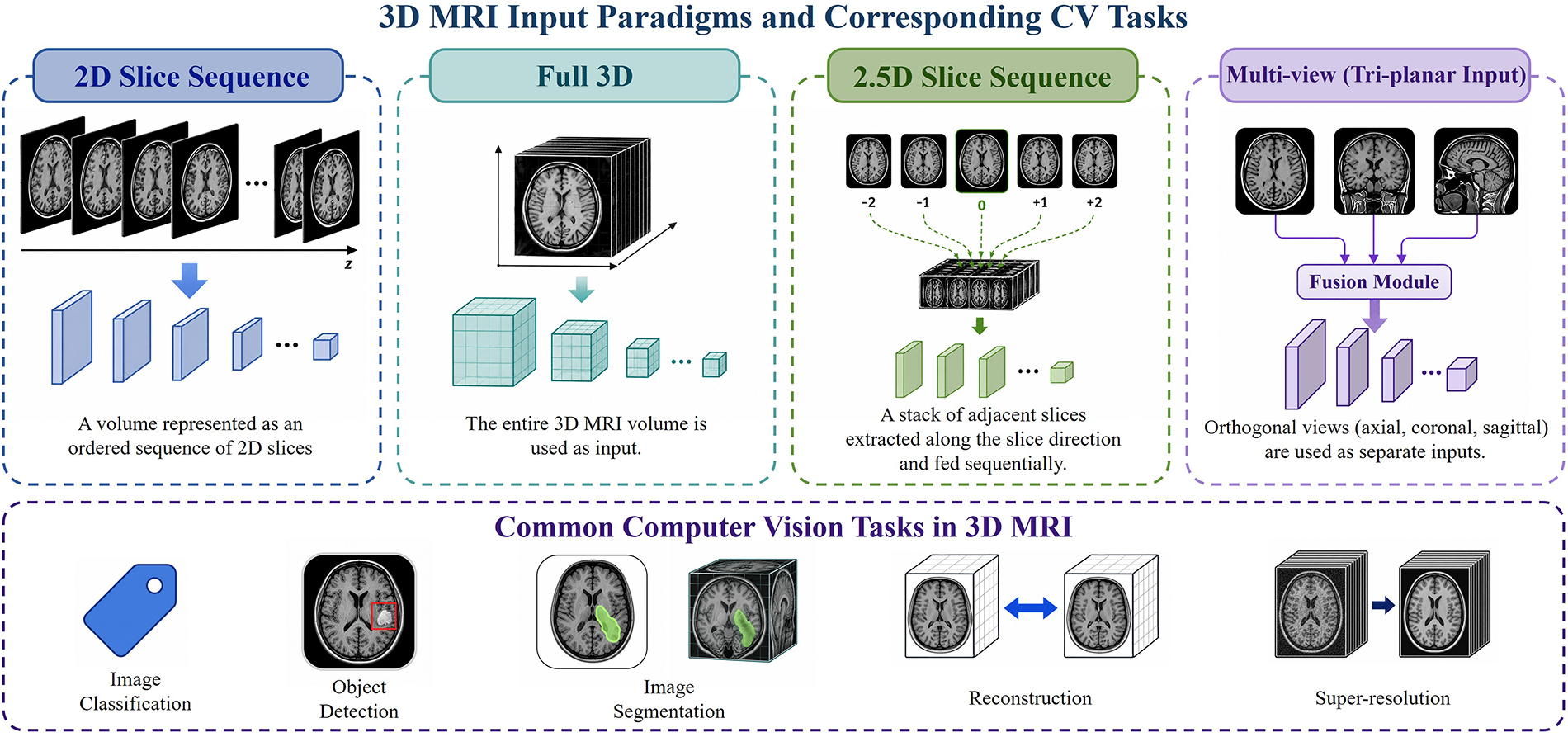
Figure 1: Schematic overview of common input paradigms for 3D MRI analysis and representative downstream computer vision tasks.

As also summarized in Fig. 1, 3D MRI supports a range of downstream computer vision tasks, including image classification [22], object detection/localization [23], image segmentation [24], reconstruction [25], and super-resolution [26]. These tasks differ in their dependence on volumetric context. Classification models often use 2D, 2.5D or multi-view, inputs to improve efficiency and robustness, whereas segmentation, reconstruction, and registration tasks usually benefit from patch-based or full 3D representations. Therefore, the input paradigm is not only an implementation choice, but also a key design factor affecting model architecture, computational efficiency, and clinical applicability.

Previous reviews have examined deep learning in MRI and medical image analysis from several angles. Lundervold and Lundervold [6] discussed deep learning in MRI across acquisition, reconstruction, segmentation, diagnosis, and clinical decision support, while Zhou et al. [27] reviewed wider developments in medical imaging, including imaging characteristics, technical trends, representative applications, and future challenges. Other reviews have focused on specific technical or clinical domains. Singh et al. [28] considered 3D deep learning for volumetric medical images across computed tomography (CT), MRI, and positron emission tomography–computed tomography (PET/CT). Wang et al. [29] summarized deep learning-based medical image synthesis, including generation, translation, and reconstruction-related applications. Gan et al. [30] reviewed medical image segmentation with attention to datasets, models, challenges, and possible solutions. Dorfner et al. [4] provided a disease-centered review of MRI-based deep learning methods for brain tumor analysis. More recently, Li et al. [19] compared 2D, 2.5D, and 3D neural network strategies for 3D medical image analysis, highlighting the influence of task settings, dataset properties, and computational constraints on dimensionality selection.

To clarify how these questions distinguish the present review from existing surveys, Table 1 compares representative reviews according to their coverage of Q1–Q5. In this context, the present review aims to provide a systematic overview of 3D MRI-based computer vision studies from the perspective of data representation, downstream task formulation, and cross-task comparison. Rather than treating 3D MRI merely as a generic data source for independent applications, we organize the literature around the relationship between volumetric input paradigms, computer vision tasks, deep learning architecture, datasets, and evaluation practices. Accordingly, this review is guided by the following research questions:

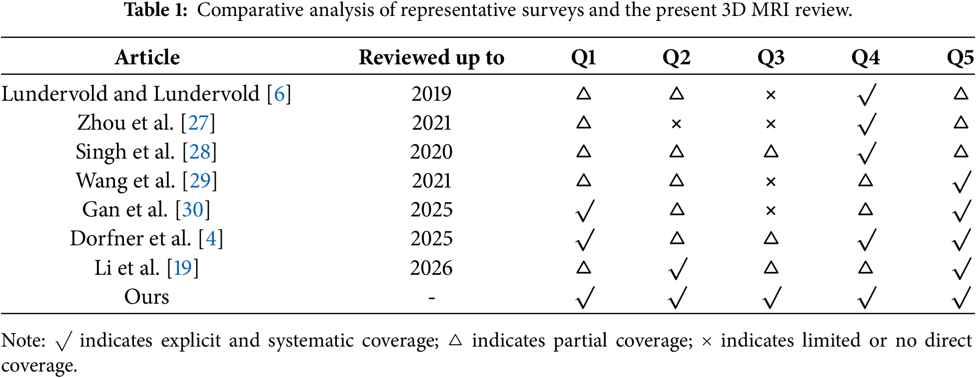
Q1: What publicly available datasets are commonly used in 3D MRI-based computer vision studies?

Q2: What input paradigms are commonly used to organize 3D MRI data for deep learning models?

Q3: How are different input paradigms matched with downstream computer vision tasks?

Q4: What are the representative downstream tasks and application scenarios in 3D MRI analysis?

Q5: What evaluation metrics and benchmarking practices are used across different tasks?

The main contributions of this review are summarized as follows. First, we provide a structured taxonomy of 3D MRI-based computer vision studies by jointly considering datasets, input paradigms, downstream tasks, model choices, and evaluation metrics. Second, we systematically analyze the major input paradigms used for 3D MRI and discuss their advantages, limitations, and task suitability. Third, we review representative downstream computer vision tasks in 3D MRI analysis, with attention to the relationship between task demands and data representation. Fourth, we summarize publicly available 3D MRI datasets and discuss how dataset characteristics influence model design and benchmarking reliability. Fifth, following a PRISMA-style literature search and screening process, this review collected studies from the Web of Science Core Collection up to May 14, 2026, identified 461 initial records, refined them to 387 task-relevant records using downstream task keywords, and finally included 178 studies after manual screening according to predefined eligibility criteria. Finally, we provide a cross-task comparative discussion to highlight how input paradigms, dataset properties, evaluation practices, and computational considerations jointly shape the development of 3D MRI-based computer vision methods.

The remainder of this review is organized as follows. Section 2 presents the literature search and study selection strategy. Section 3 summarizes publicly available datasets and application scenarios in 3D MRI analysis. Section 4 discusses major input paradigms for 3D MRI representation and compares their technical characteristics. Section 5 reviews downstream computer vision tasks and representative deep learning approaches. Section 6 discusses current challenges and future directions. Finally, Section 7 concludes the review.

2  Literature Search and Study Classification

2.1 Search Strategy and Screening Procedure

To establish a structured corpus of recent studies on computer vision methods for 3D MRI, we conducted a literature search in the Web of Science Core Collection. The search was completed on May 14, 2026. The review was intentionally restricted to peer-reviewed journal articles indexed in the Web of Science Core Collection. This scope was selected to construct a reproducible archival corpus with relatively consistent bibliographic metadata and sufficiently detailed reporting of datasets, preprocessing procedures, input representations, model designs, and evaluation protocols. Conference proceedings, preprints, reviews and study protocols were not considered eligible for the final corpus.

The search strategy was designed to retrieve studies satisfying three conceptual conditions: the use of 3D or volumetric MRI data, the involvement of artificial intelligence or computer vision methods, and the presence of clearly described data-processing or input-representation strategies.

The following topic search query was used:

TS = ((“3D MRI” OR “three-dimensional MRI” OR “volumetric MRI” OR “3D magnetic resonance imaging” OR “volumetric magnetic resonance imaging” OR “multi-modal MRI” OR “multimodal MRI”) AND (“deep learning” OR “machine learning” OR “artificial intelligence” OR “neural network” OR “convolutional neural network” OR CNN OR transformer OR “computer vision”) AND (“preprocess” OR “data processing” OR “input representation” OR “input strategy” OR “2.5D” OR “3D” OR “patch-based” OR “slice-based” OR “multi-view”)) AND PY = (2021–2026).

The first group of terms identified studies involving 3D MRI, volumetric MRI, or multimodal MRI data. The second group restricted the results to studies involving artificial intelligence, machine learning, deep learning, neural networks, or computer vision. The third group was used to identify studies reporting data preprocessing, input representation, or data-organization strategies, including 2.5D, full 3D, patch-based, slice-based, and multi-view designs.

The search was restricted to peer-reviewed journal articles published between 2021 and 2026. Conference proceedings, preprints, reviews, and retracted publications were outside the predefined scope of the review. After applying the database-level publication-year and document-type filters, 461 records were retrieved. The titles and abstracts of all retrieved records were then manually screened for preliminary relevance. At this stage, 74 records were excluded. These records included studies that did not address an eligible MRI-based computer vision task, retracted publications, study protocols, and review or overview articles that remained in the retrieved results despite the database-level document-type filtering. After this title-and-abstract screening stage, 387 records remained for detailed eligibility assessment.

The remaining 387 records were assessed in detail according to the predefined eligibility criteria. Four inclusion criteria were applied. First, the study had to involve 3D MRI or volumetric MRI data rather than exclusively two-dimensional MRI images without volumetric context. Second, the dataset used in the study had to be publicly available. Third, the study had to address an explicit MRI-based computer vision task, including classification or recognition, detection or localization, segmentation or parcellation, registration, reconstruction or restoration, super-resolution, or another clearly defined image-based prediction task. Fourth, the input representation or data-organization strategy had to be clearly specified, including 2D slice-based, 2.5D, full 3D, patch-based volumetric, or multi-view designs.

Based on these criteria, 209 records were excluded during detailed eligibility assessment. Finally, 178 studies were included in this review. The screening and selection procedures were conducted in multiple stages following PRISMA’s recommendations for systematic reviews [31]. The literature identification, screening, eligibility assessment, and final inclusion process is summarized in Fig. 2. PRISMA checklists are available in the Supplementary Material.

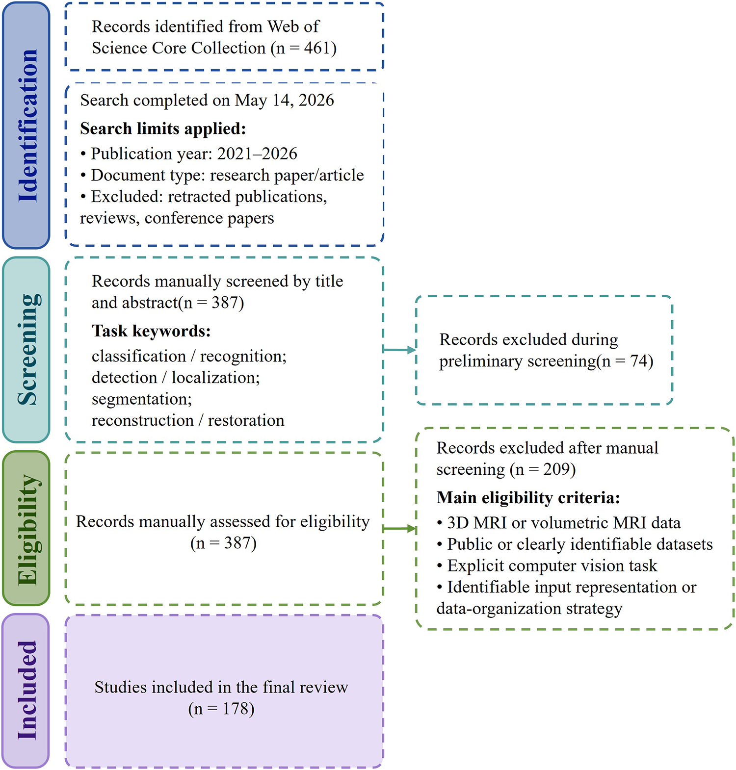
Figure 2: PRISMA-style flow diagram of literature identification, screening, eligibility assessment, and final inclusion.

2.2 Classification Framework

After the final set of 178 studies was determined, each article was further reviewed and categorized according to three dimensions: dataset family, input paradigm, and downstream computer vision task. This classification framework was designed to provide a structured basis for the subsequent analysis of public datasets, volumetric input strategies, network design patterns, and task-specific applications in 3D MRI-based computer vision.

The first dimension was the dataset family. Major dataset families identified in the reviewed corpus included Brain Tumor Segmentation (BraTS), Alzheimer’s Disease Neuroimaging Initiative (ADNI), Open Access Series of Imaging Studies (OASIS), IXI, Osteoarthritis Initiative (OAI), fastMRI, Human Connectome Project (HCP), Anatomical Tracings of Lesions After Stroke (ATLAS), Medical Segmentation Decathlon (MSD) Brain Tumor, and Minimal Interval Resonance Imaging in Alzheimer’s Disease (MIRIAD). These datasets cover different anatomical regions, disease contexts, and imaging objectives. In this review, dataset-family annotation was used primarily to describe the methodological and application background of the included studies, while more detailed dataset characteristics are discussed in Section 3.

The second dimension was the input paradigm. In this review, the main input paradigms were grouped into four categories: 2D slice sequence, 2.5D slice sequence, full 3D volume, and multi-view or tri-planar input. A 2D slice-sequence strategy processes volumetric MRI as a set or sequence of two-dimensional slices. A 2.5D strategy incorporates adjacent slices or limited through-plane information to provide partial volumetric context. A full 3D strategy directly processes the entire volume or volumetric subregions using three-dimensional operations. A multi-view or tri-planar strategy integrates information from different anatomical planes, usually axial, coronal, and sagittal views.

The third dimension was the downstream computer vision task. The reviewed studies were grouped into four broad task categories: detection/diagnosis, segmentation, reconstruction, and super-resolution. Detection/diagnosis was used as an umbrella category for studies focusing on disease classification, abnormality detection, lesion localization, clinical status prediction, or computer-aided diagnosis. Segmentation referred to studies aiming to delineate anatomical structures, tissues, organs, tumors, or lesions. Reconstruction included studies that recovered MRI images or volumes from undersampled, incomplete, corrupted, or transformed acquisition data. Super-resolution referred to studies that enhanced spatial resolution or generated high-resolution MRI representations from low-resolution inputs.

When a study involved multiple input paradigms or downstream tasks, a primary or “dominant” setting was assigned for the article-level classification. The dominant task was defined as the task corresponding to the principal research objective, main experimental results, and primary conclusion. The dominant input paradigm was determined from the representation actually received by the principal model in the main experiment. For example, a study using volumetric patches processed by 3D operations was classified as full 3D, while patch-based processing was retained as an implementation-level characteristic. Similarly, a study combining segmentation with auxiliary classification was categorized as segmentation when lesion delineation constituted the primary endpoint. Ambiguous cases were re-examined against the title, abstract, methods, principal experimental tables, and conclusions before the final classification was assigned.

The dominant-setting classification was used to provide a concise article-level summary of the 178-study corpus. It should be distinguished from the dataset–input–task flow records used for the Sankey analysis in Section 2.3. In the Sankey analysis, one article could contribute multiple dataset-specific flow records when the same principal method was evaluated on multiple publicly available datasets.

2.3 Overview of Dataset–Input–Task Relationships

To examine how datasets, input paradigms, and downstream tasks were associated across the included literature, we constructed a set of literature-level dataset–input paradigm–task flow records. The unit of analysis in this section was a flow record rather than a unique article. For each included study, the dominant input paradigm and downstream task were determined according to the criteria described in Section 2.2, whereas all publicly available datasets used to evaluate the principal method were retained. Consequently, an article evaluated on multiple datasets could contribute more than one flow record, although its dominant input paradigm and task remained unchanged.

Each flow record initially contained a specific dataset name or release, an input paradigm, and a downstream task. Dataset versions belonging to the same benchmark family were subsequently consolidated for visualization. For example, different BraTS releases were displayed under the BraTS family, and different OASIS releases were displayed under the OASIS family.

To focus Fig. 3 on recurrent patterns, grouped dataset–input paradigm–task relations supported by only one article were omitted from the visualization. After dataset-family consolidation and low-frequency relation filtering, 42 recurrent relation types were retained. These relation types comprised 265 literature-level flow records. The value of 265 represents the total number of retained article–dataset relations connecting a grouped dataset family, a dominant input paradigm, and a dominant downstream task. The complete list of article-level relations used to construct the Sankey diagram is provided in the Supplementary Materials.

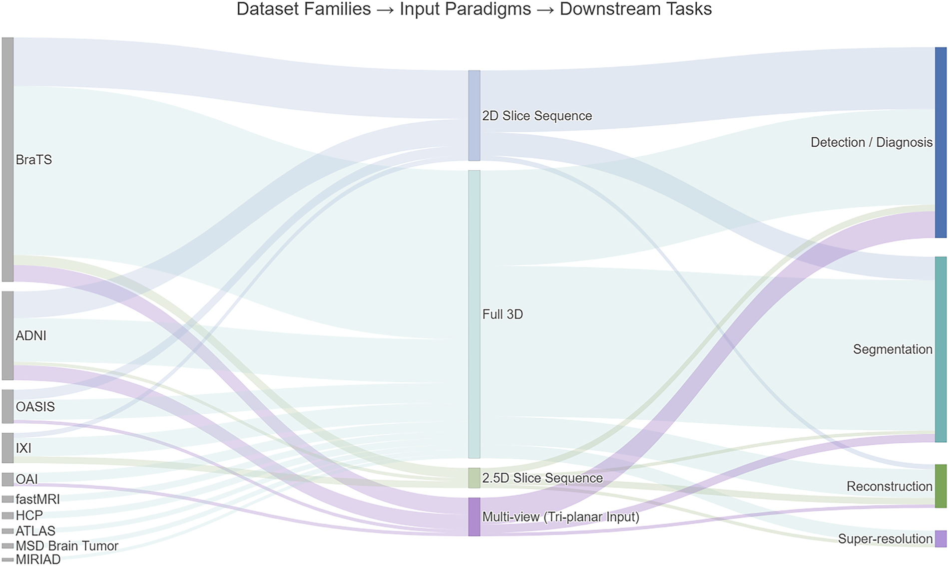
Figure 3: Sankey diagram showing the grouped relationships among dataset families, input paradigms, and downstream computer vision tasks.

Fig. 3 shows that the retained relations were concentrated in a limited number of public benchmark families. BraTS contributed 146 flow records and ADNI contributed 51, whereas OASIS, IXI, OAI, HCP, fastMRI, ATLAS, MSD Brain Tumor, and MIRIAD occurred less frequently. The largest recurrent relation was BraTS–Full 3D–Segmentation, followed by BraTS–Full 3D–Detection/Diagnosis. These patterns are consistent with the volumetric nature of brain tumor analysis, in which lesion extent, subregion structure, and spatial heterogeneity are commonly modeled in three dimensions. ADNI relations were concentrated primarily in detection and diagnosis tasks and included full 3D, 2D slice-based, and multi-view representations, reflecting its frequent use in Alzheimer’s disease classification, mild cognitive impairment prediction, and disease-stage modeling.

At the input-paradigm level, full 3D was the most frequent representation, accounting for 174 of the 265 retained flow records. Detection/diagnosis and segmentation formed the two largest downstream task groups, whereas reconstruction and super-resolution appeared less frequently in the retained relations. Overall, Fig. 3 indicates that recent 3D MRI computer vision research within the reviewed corpus has been organized around several recurring combinations: brain MRI benchmarks, particularly BraTS and ADNI; full 3D representations; and detection/diagnosis or segmentation tasks. The continued presence of 2D, 2.5D, and multi-view relations also indicates that input-paradigm selection remains dependent on task requirements, dataset characteristics, annotation availability, and computational constraints. Publication years and structured methodological information for all included studies are provided in the Supplementary Materials.

3  Dataset Families and Research Targets

3.1 Overview of Dataset Families by Anatomical Region and Research Objective

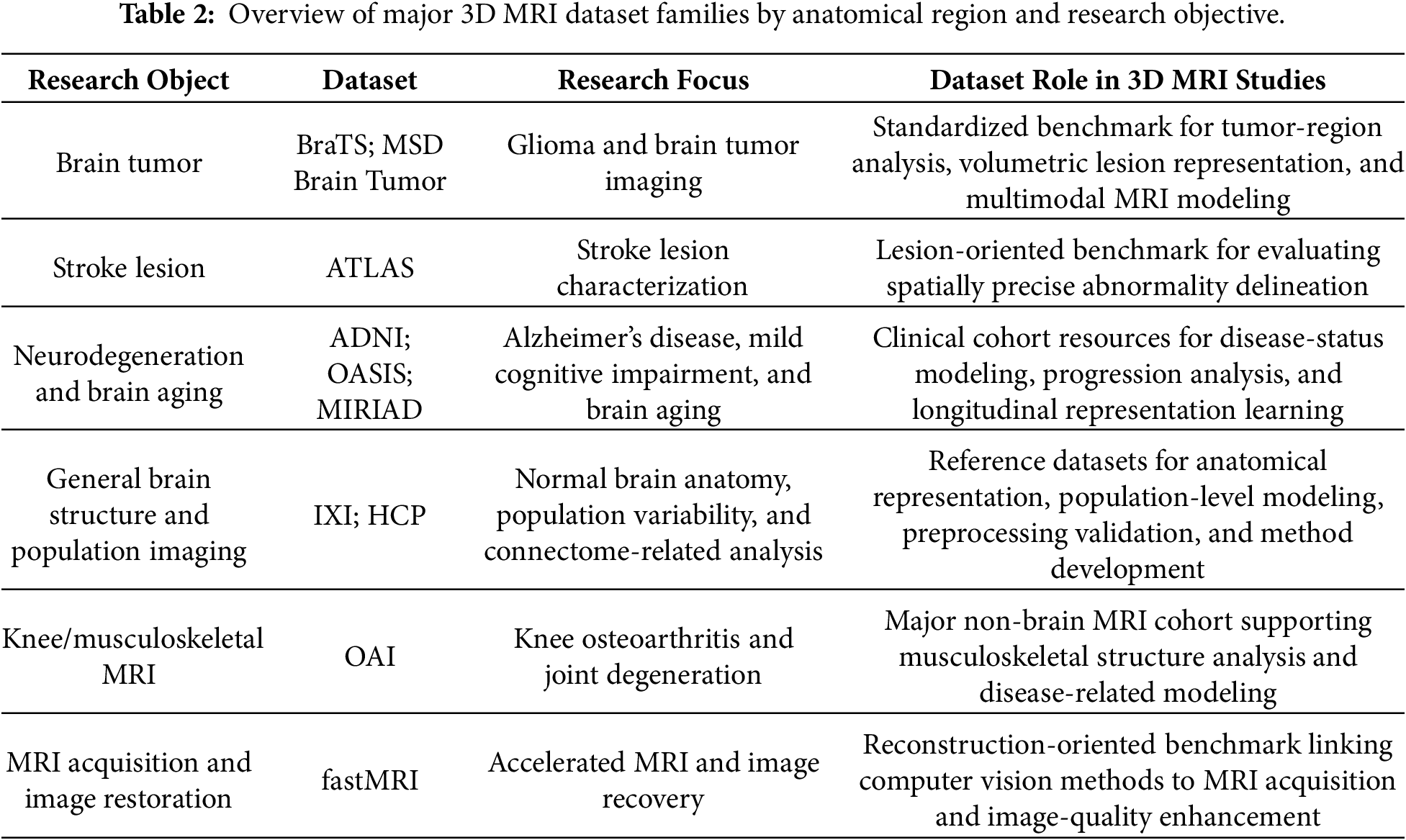
Compared with natural image benchmarks, MRI datasets are more closely tied to anatomical region, disease context, acquisition protocol, imaging sequence, and annotation type. As a result, each dataset family tends to support a particular set of methodological and clinical questions. BraTS and MSD Brain Tumor, for example, are primarily used in multimodal brain tumor imaging [32–36]. ADNI, OASIS, and MIRIAD are more closely linked to neurodegenerative disease, cognitive decline, and brain aging [37–41]. OAI represents a musculoskeletal MRI cohort for knee osteoarthritis research [42–44], whereas fastMRI is designed mainly for MRI reconstruction and image recovery rather than disease-centered image interpretation [45,46].

To provide a high-level overview, the major dataset families identified in this review were grouped according to anatomical region and research objective. At this stage, dataset families are discussed at the family level rather than by individual release or version. For instance, different BraTS challenge releases are collectively referred to as the BraTS family, and OASIS-1, OASIS-2, and OASIS-3 are summarized as the OASIS family. This grouping strategy is useful for revealing the broader role of each dataset family before introducing their version-specific details in subsequent subsections.

Fig. 4 illustrates the anatomy–dataset map of the major 3D MRI dataset families. The reviewed datasets can be broadly divided into six categories: brain tumor datasets, stroke lesion datasets, neurodegeneration and brain aging datasets, general brain structure and population imaging datasets, knee or musculoskeletal MRI datasets, and MRI acquisition or image-restoration datasets. This organization highlights that the reviewed literature is dominated by brain MRI resources, but also includes important non-brain and reconstruction-oriented datasets.

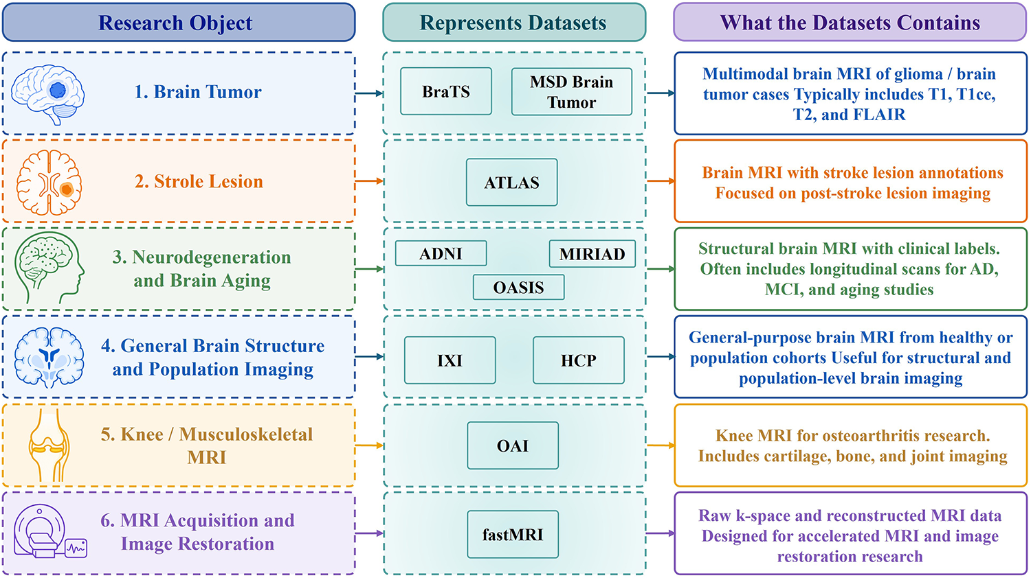
Figure 4: Anatomy-dataset-map of major 3D MRI dataset families.

Brain tumor datasets, represented by the BraTS family and MSD Brain Tumor, typically contain multimodal MRI scans of glioma or brain tumor cases. Stroke lesion imaging is mainly represented by ATLAS. Unlike tumor datasets, ATLAS focuses on post-stroke lesion patterns and provides brain MRI with lesion annotations. Neurodegeneration and brain aging datasets include ADNI, OASIS, and MIRIAD. These datasets mainly contain structural brain MRI, often combined with clinical diagnosis, cognitive measurements, demographic information, biomarker data, or longitudinal follow-up. General brain structure and population imaging datasets, such as IXI and HCP, are less disease-specific. They primarily provide structural or multimodal brain MRI from healthy or population-level cohorts. OAI represents a distinct musculoskeletal MRI resource in the reviewed corpus. It focuses on knee osteoarthritis and includes knee MRI together with clinical and imaging-related information. Finally, fastMRI differs from most other dataset families because its primary focus is MRI acquisition and image restoration. Rather than being organized around a specific disease label, fastMRI provides raw k-space data and reconstructed MRI images for accelerated MRI reconstruction.

Preprocessing conditions also vary across these dataset families. Some public benchmarks provide images that have already undergone steps such as registration, skull stripping, resampling, or intensity standardization, whereas others retain data closer to their original acquisition form. These differences affect the spatial and intensity information available to downstream models and may influence the suitability of different input paradigms. Because preprocessing is often inherited from the released dataset rather than introduced as a separate methodological contribution, this review treats it as an upstream dataset condition rather than an independent comparison dimension. Table 2 summarizes the major dataset families according to anatomical region, research object, data content, and their roles in 3D MRI-based computer vision studies.

3.2 Brain Tumor Datasets

Brain tumor datasets represent one of the most mature and widely used dataset categories in 3D MRI-based computer vision. The reviewed corpus contains two principal brain-tumor dataset families: BraTS family and MSD Brain Tumor. These datasets are centered on glioma or brain tumor imaging and usually provide multimodal brain MRI volumes together with tumor-region annotations.

The methodological importance of brain tumor datasets lies in three aspects. First, brain tumors are inherently three-dimensional lesions with irregular morphology, heterogeneous intensity patterns, and variable anatomical locations. This makes them particularly suitable for evaluating volumetric feature extraction and spatial-context modeling. Second, multimodal MRI sequences provide complementary information about tumor tissue composition.

Fig. 5 provides a representative example of multimodal brain tumor MRI data used in this review. The example is selected from BraTS 2020 and illustrates the four commonly used MRI modalities, namely T1, T1ce, T2, and FLAIR, together with tumor-region annotations. Although MSD Brain Tumor is also included in this dataset category, it is not separately visualized here because the MSD Brain Tumor task was derived from brain tumor segmentation data associated with the BraTS 2016 and BraTS 2017 challenges. Therefore, it shares a similar multimodal MRI configuration and annotation setting with BraTS-style datasets.

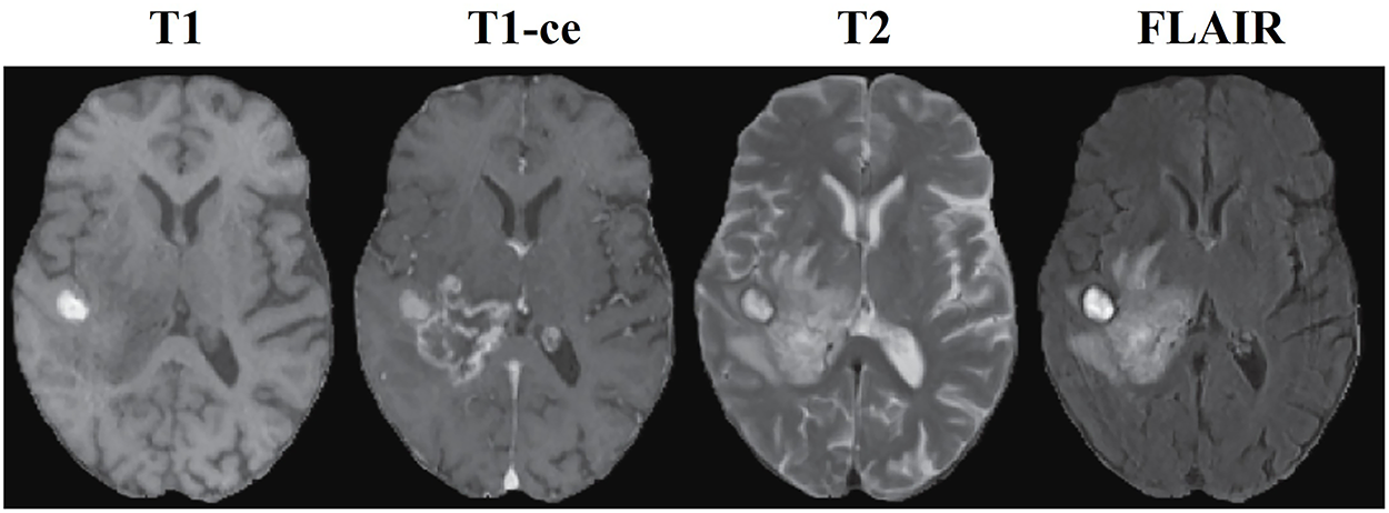
Figure 5: Representative examples of multimodal brain tumor MRI data and tumor-region annotations (BraTS 2020).

3.2.1 BraTS Family

The Brain Tumor Segmentation challenge, commonly known as BraTS, has become a benchmark family for brain tumor segmentation in multimodal MRI. Since its early releases, BraTS has provided a standardized platform for evaluating computational methods for glioma segmentation. The dataset family is mainly composed of preoperative brain MRI scans from glioma patients, together with expert-annotated tumor subregions [47–49]. In general, access to BraTS data is not fully open for direct download; researchers usually need to apply for data access through the official BraTS Synapse portal, available at https://www.synapse.org/brats, and obtain approval before downloading the datasets.

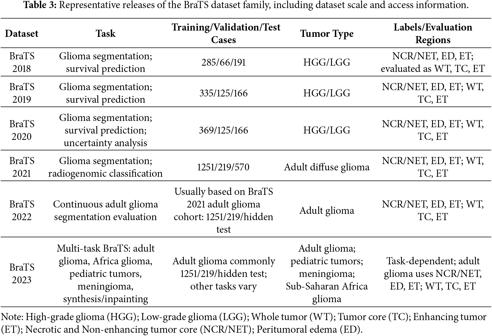
A typical BraTS case contains four MRI modalities: native T1-weighted, contrast-enhanced T1-weighted, T2-weighted, and FLAIR images. Together, they provide complementary anatomical and tumor-related information. BraTS is also widely used because of its detailed tumor annotations. The masks usually distinguish enhancing tumor, peritumoral edema, and necrotic or non-enhancing tumor core. For evaluation, these labels are often combined into whole tumor, tumor core, and enhancing tumor regions. This structure supports both overall lesion segmentation and more detailed subregion analysis. Across yearly releases, BraTS has expanded in sample size, cohort diversity, and task design. Table 3 summarizes representative BraTS releases frequently used in recent 3D MRI-based computer vision studies.

3.2.2 MSD Brain Tumor

The brain tumor subset of Medical Segmentation Decathlon (MSD), usually referred to as Task01_BrainTumour, is closely related to multimodal glioma MRI segmentation [50]. The dataset is distributed as part of the Medical Segmentation Decathlon and can be accessed through the official MSD website: http://medicaldecathlon.com/. Since the dataset follows the MSD framework, it is commonly distributed in a standardized NIfTI format, which makes it compatible with many 3D medical image segmentation pipelines such as U-Net variants, nnU-Net, and transformer-based volumetric segmentation models [51]. Table 4 summarizes the key information of MSD Brain Tumor, including its task setting, data scale, annotation structure and relationship with the BraTS challenge datasets.

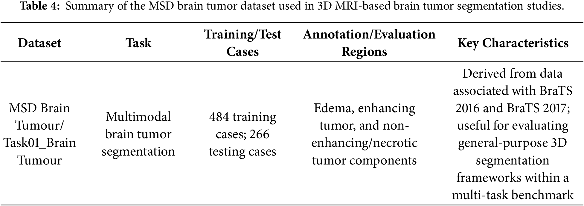
Compared with BraTS, MSD Brain Tumor is usually discussed from a slightly different perspective. BraTS is a disease-specific benchmark with a long challenge history and version-specific releases, whereas MSD Brain Tumor is one task within a broader multi-domain benchmark.

3.3 Stroke Lesion Datasets

ATLAS

ATLAS is a public stroke neuroimaging dataset designed for the development and evaluation of automated lesion segmentation algorithms [52,53]. The dataset provides T1-weighted brain MRI scans together with manually annotated stroke lesion masks. A representative example of ATLAS-style data is shown in Fig. 6. The upper row presents T1-weighted axial brain MRI slices, while the lower row shows the corresponding lesion annotations overlaid in red.

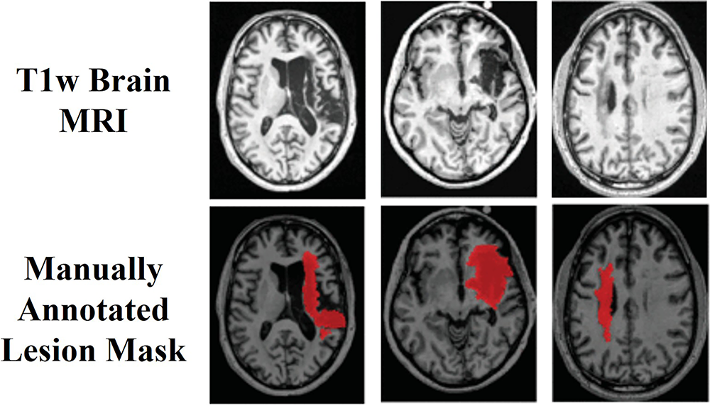
Figure 6: Representative examples of stroke lesion MRI data and manually annotated lesion masks.

The ATLAS dataset has evolved across releases, as summarized in Table 5. More detailed information about the dataset construction, preprocessing pipeline, lesion tracing protocol, and challenge organization can be found in the ATLAS v1.2 data descriptor [52] and ATLAS v2.0 data descriptor [53]. ATLAS data can be accessed through the International Neuroimaging Data-Sharing Initiative platform at https://fcon_1000.projects.nitrc.org/indi/retro/atlas.html.

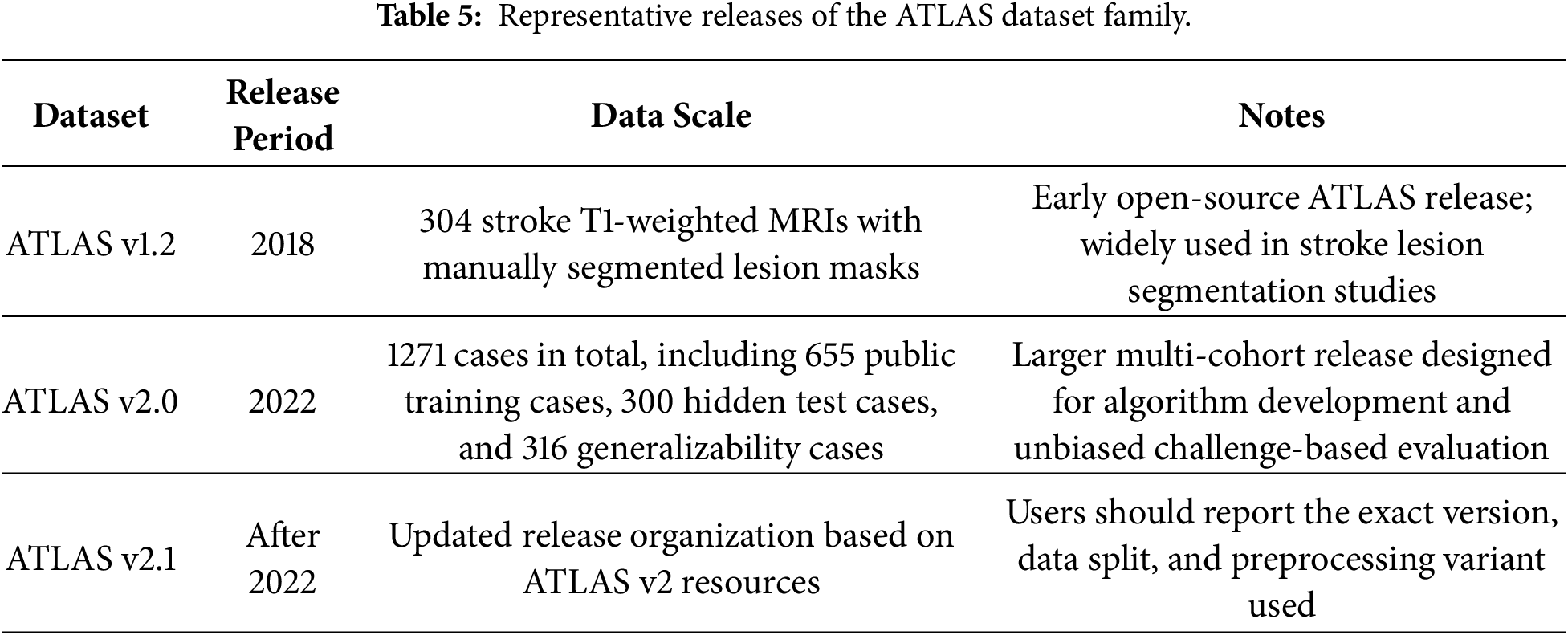
Because stroke lesions may be small, irregular, sparse, and distributed across different anatomical locations, ATLAS is particularly useful for evaluating the ability of segmentation models to handle foreground–background imbalance and heterogeneous lesion boundaries.

3.4 Neurodegeneration and Brain Aging Datasets

Neurodegeneration datasets differ from lesion-centered benchmarks because their labels are primarily assigned at the subject or visit level and are often accompanied by longitudinal clinical information. The three principal resources examined here are ADNI, OASIS, and MIRIAD.

Fig. 7 presents representative structural MRI examples from cognitively normal controls in ADNI, OASIS, and MIRIAD. The main value of these datasets lies in the associated clinical labels, longitudinal records, and biomarker information, rather than visually obvious focal abnormalities.

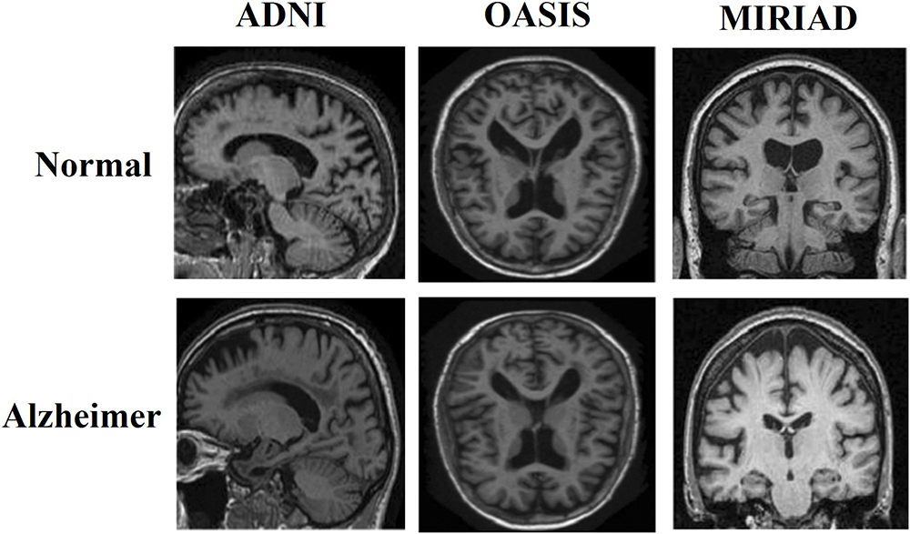
Figure 7: Representative structural MRI examples from cognitively normal control groups in ADNI, OASIS, and MIRIAD.

3.4.1 ADNI Family

ADNI supports Alzheimer’s disease classification, conversion prediction, disease staging, and longitudinal progression modeling [54–56]. Most ADNI-based MRI studies use structural T1-weighted brain MRI as the main input. Depending on the task, MRI may also be combined with PET, cerebrospinal fluid biomarkers, genetic data, demographic variables, or neuropsychological scores [57].

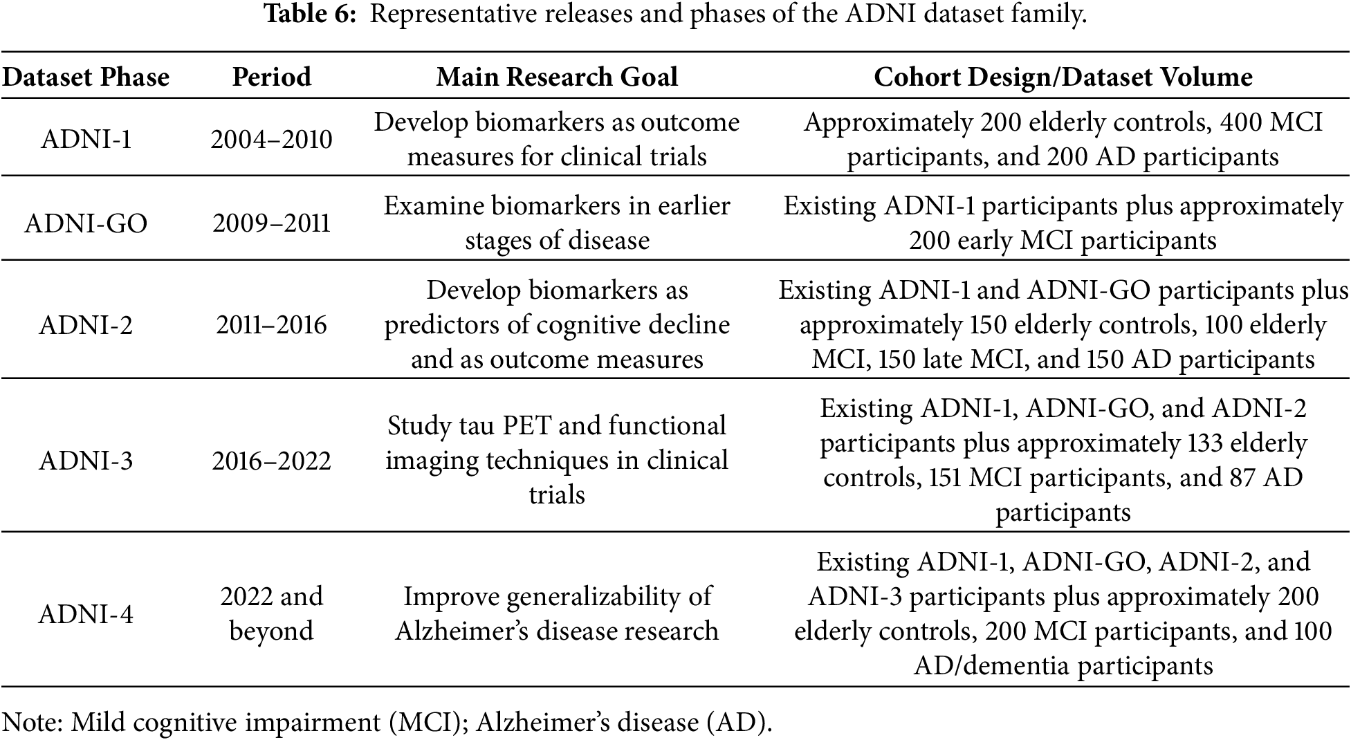
ADNI data are available through the Laboratory of Neuro Imaging (LONI)/ADIN portal (https://adni.loni.usc.edu/about/), with registration and data-use approval required. As shown in Table 6, ADNI should be regarded as a dataset family because ADNI-1, ADNI-GO, ADNI-2, ADNI-3, and later releases differ in cohort design, imaging protocols, available modalities, and follow-up structure.

3.4.2 OASIS Family

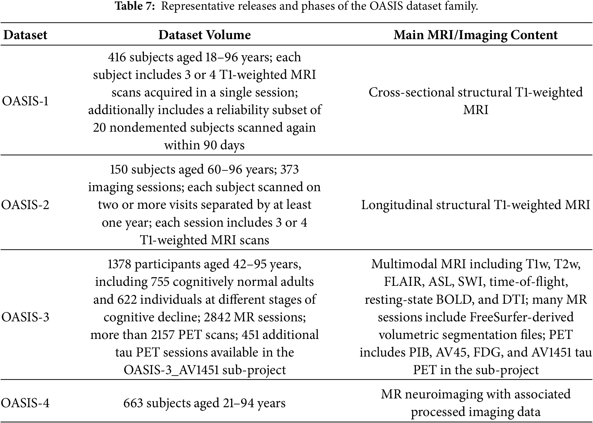
The Open Access Series of Imaging Studies, or OASIS, is another widely used dataset family for brain aging and dementia research. The OASIS family includes several releases, commonly referred to as OASIS-1, OASIS-2, OASIS-3, and OASIS-4, each with different cohort structures and imaging content [58–60]. OASIS data can be accessed through the official OASIS data portals (https://sites.wustl.edu/oasisbrains/). As summarized in Table 7, the OASIS family covers both cross-sectional and longitudinal study designs.

3.4.3 MIRIAD

The Minimal Interval Resonance Imaging in Alzheimer’s Disease dataset, commonly known as MIRIAD, is a longitudinal MRI dataset designed for Alzheimer’s disease research [61]. MIRIAD data are available through the official project route specified by the dataset provider, including the UCL MIRIAD project page and the NITRC distribution page (https://www.nitrc.org/projects/miriad). Table 8 summarizes the role of MIRIAD as a neurodegeneration and brain aging dataset.

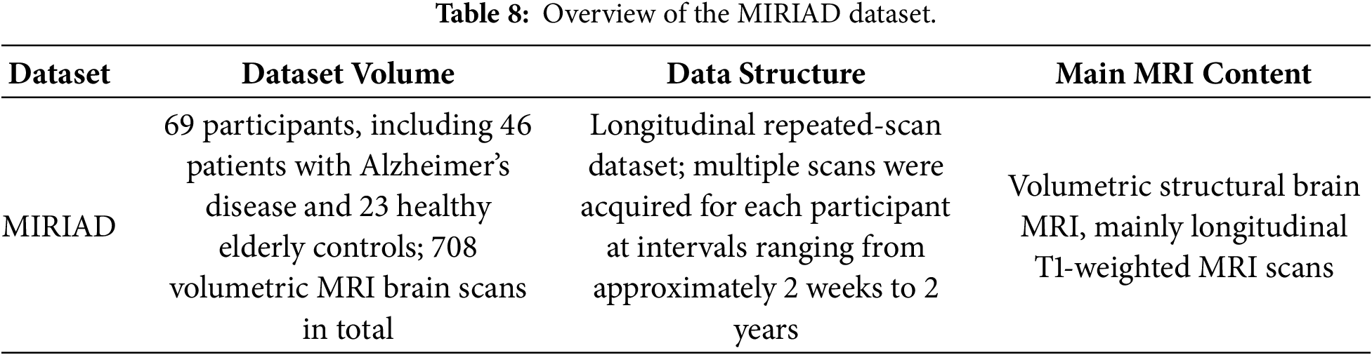
The role of MIRIAD differs from that of large-scale challenge datasets. It is not usually used as a primary benchmark for training large deep learning models from scratch. Instead, it is more often useful for testing robustness, reproducibility, longitudinal consistency, and external validation. Because of its relatively limited cohort size and repeated-measure design, MIRIAD is better suited for evaluating measurement stability and biologically plausible longitudinal change than for training high-capacity 3D deep models de novo.

3.5 General Brain Structure and Population Imaging Datasets

General brain structure and population imaging datasets provide reference resources for 3D MRI-based computer vision. They usually contain structural or multimodal brain MRI from healthy volunteers or population-level cohorts, and are mainly used for anatomical representation learning, preprocessing validation, registration, segmentation, reconstruction, super-resolution, and population-level analysis.

In this review, this category is mainly represented by IXI and Human Connectome Project (HCP). IXI is an accessible structural MRI dataset often used for method validation, whereas HCP provides high-quality multimodal neuroimaging data for large-scale studies of brain structure, function, and connectivity. Since both datasets mainly show general brain anatomy and do not include distinctive lesion masks or disease-specific annotations, no representative image panel is provided. This subsection therefore focuses on dataset scale, imaging content, access route, and methodological role.

3.5.1 IXI

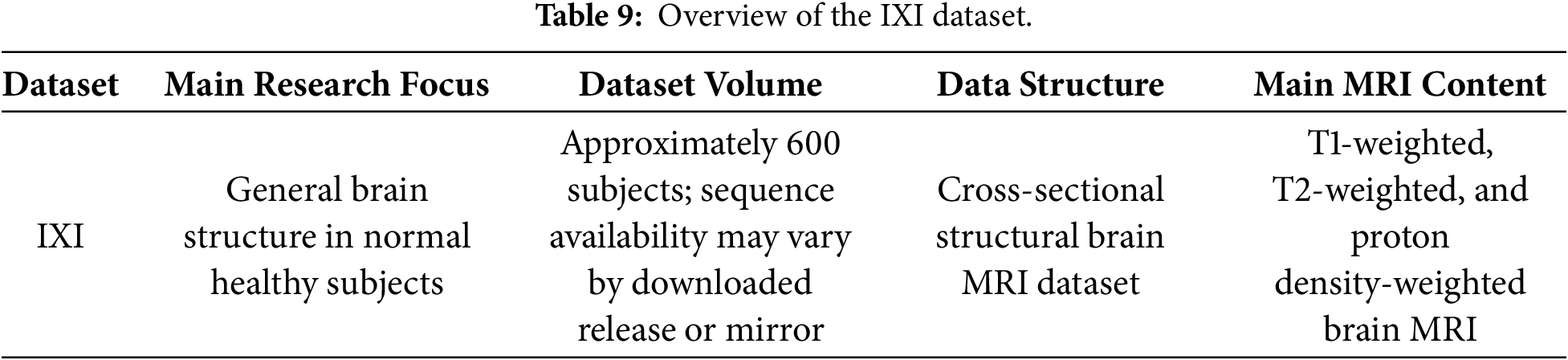
IXI is a public brain MRI dataset containing approximately 600 healthy subjects collected from multiple hospitals in London [62]. It provides commonly used structural MRI sequences, including T1-weighted, T2-weighted, and proton density-weighted images.

IXI is commonly used for structural brain representation, modality translation, segmentation, registration, reconstruction, and super-resolution. Its value lies less in clinical labels and more in providing a clean reference dataset for evaluating image-processing pipelines and anatomical representation learning. IXI data can be accessed through the official webpage: https://brain-development.org/ixi-dataset/. As summarized in Table 9, IXI mainly serves as a general-purpose structural brain MRI dataset for method validation rather than disease diagnosis.

From a methodological perspective, IXI is particularly relevant to studies that require relatively standardized brain MRI data without strong disease-specific labels. The main limitation of IXI is that it is not a large-scale clinical cohort and does not provide rich disease labels or longitudinal follow-up.

3.5.2 HCP

The Human Connectome Project, commonly known as HCP, is a large-scale neuroimaging resource designed to study human brain structure, function, and connectivity [63,64]. Recent work has used HCP for anatomical modeling, representation learning, multimodal analysis, segmentation, and reconstruction.

In this review, HCP mainly refers to the WU-Minn HCP Young Adult S1200 release, particularly the structural MRI subset containing 1113 subjects as summarized in Table 10.

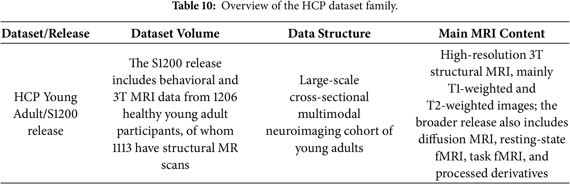
HCP data are accessed through the HCP Young Adult project page (https://www.humanconnectome.org/study/hcp-young-adult). HCP has several advantages for 3D MRI-based computer vision. First, its high-resolution structural MRI makes it useful for detailed anatomical representation learning. Second, its multimodal imaging structure supports models that integrate structural, diffusion, and functional information. Third, the relatively standardized acquisition and preprocessing pipelines make it suitable for methodological studies that require high-quality input data.

3.6 Knee/Musculoskeletal MRI Datasets

Unlike brain MRI, knee MRI focuses on joint structures such as cartilage, bone, meniscus, ligaments, and surrounding soft tissues, which are closely related to degenerative joint diseases and require different analysis strategies. In this review, this category is mainly represented by the Osteoarthritis Initiative (OAI). Fig. 8 shows representative knee MRI examples to illustrate the anatomical context of OAI-style musculoskeletal imaging.

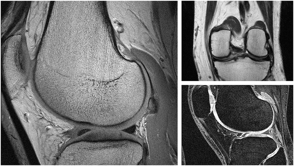
Figure 8: Representative knee MRI examples from the Osteoarthritis Initiative (OAI).

3.6.1 OAI

Applications based on OAI include osteoarthritis diagnosis, progression prediction, cartilage segmentation, and quantitative morphology analysis [65,66]. OAI includes standardized 3.0 T knee MRI protocols with sagittal, coronal, or axial acquisitions depending on the selected visit and sequence. The dataset also provides radiographic assessments and rich clinical variables, allowing image-derived features to be linked with symptoms, radiographic severity, pain scores, functional outcomes, and disease progression. OAI data can be accessed through the National Institutes of Health (NIH) NIMH Data Archive (NDA) OAI portal: https://nda.nih.gov/oai/. As summarized in Table 11, OAI extends 3D MRI-based computer vision from neuroimaging to musculoskeletal imaging.

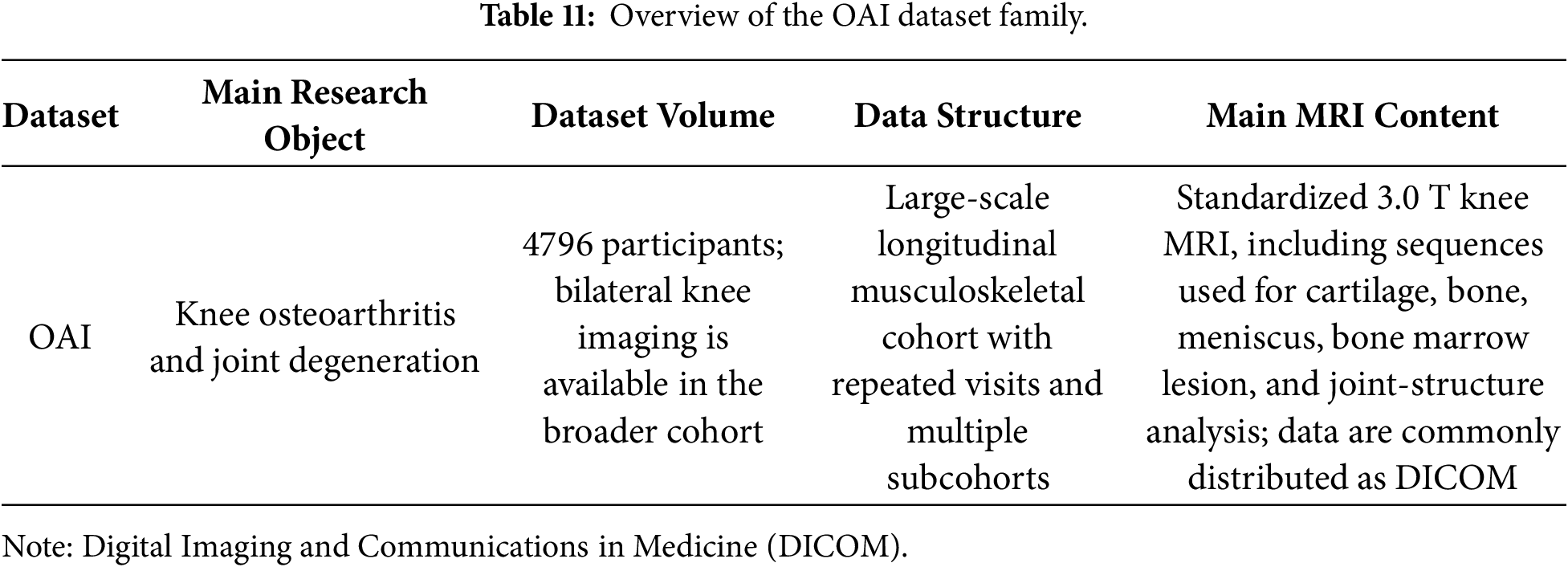
OAI introduces challenges that differ from brain MRI analysis because knee MRI contains thin cartilage layers, curved bone surfaces, menisci, ligaments, and other small soft-tissue structures, requiring high spatial precision. It is also suitable for comparing different input paradigms, including full 3D, slice-based, patch-based, and region of interest (ROI)-based strategies, especially for localized structures such as cartilage, meniscus, bone marrow lesions, and subchondral bone.

3.7 MRI Acquisition and Image Restoration Datasets

MRI acquisition and image restoration datasets form a distinct category in 3D MRI-based computer vision. Unlike disease-centered datasets, they focus on recovering high-quality MRI from raw, undersampled, noisy, or degraded acquisition data rather than on diagnosis or lesion annotation. In this review, fastMRI is the main representative dataset, supporting accelerated MRI reconstruction, image restoration, super-resolution, artifact reduction, and data-driven image-quality enhancement.

Since fastMRI includes multiple anatomical regions, such as knee, brain, prostate, and breast MRI, it is better regarded as a dataset family with different anatomical subsets rather than a single homogeneous cohort. Fig. 9 illustrates this cross-anatomical coverage.

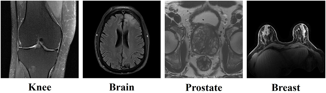
Figure 9: Representative fastMRI examples from different anatomical regions, including knee, brain, prostate, and breast MRI.

3.7.1 fastMRI

fastMRI is a large public MRI reconstruction dataset developed by NYU Langone Health and Facebook AI Research for machine learning-based accelerated MRI [67–70]. Its key feature is the availability of deidentified raw k-space data, enabling models to learn reconstruction from undersampled frequency-domain measurements rather than only using reconstructed images.

As summarized in Table 12, fastMRI includes several anatomical subsets, including knee, brain, prostate, and breast MRI. Its core content is raw acquisition data and reconstructed images, rather than clinical labels or voxel-level masks, making it different from most diagnosis- or segmentation-oriented datasets. Data are available through the official fastMRI portal (https://fastmri.med.nyu.edu/).

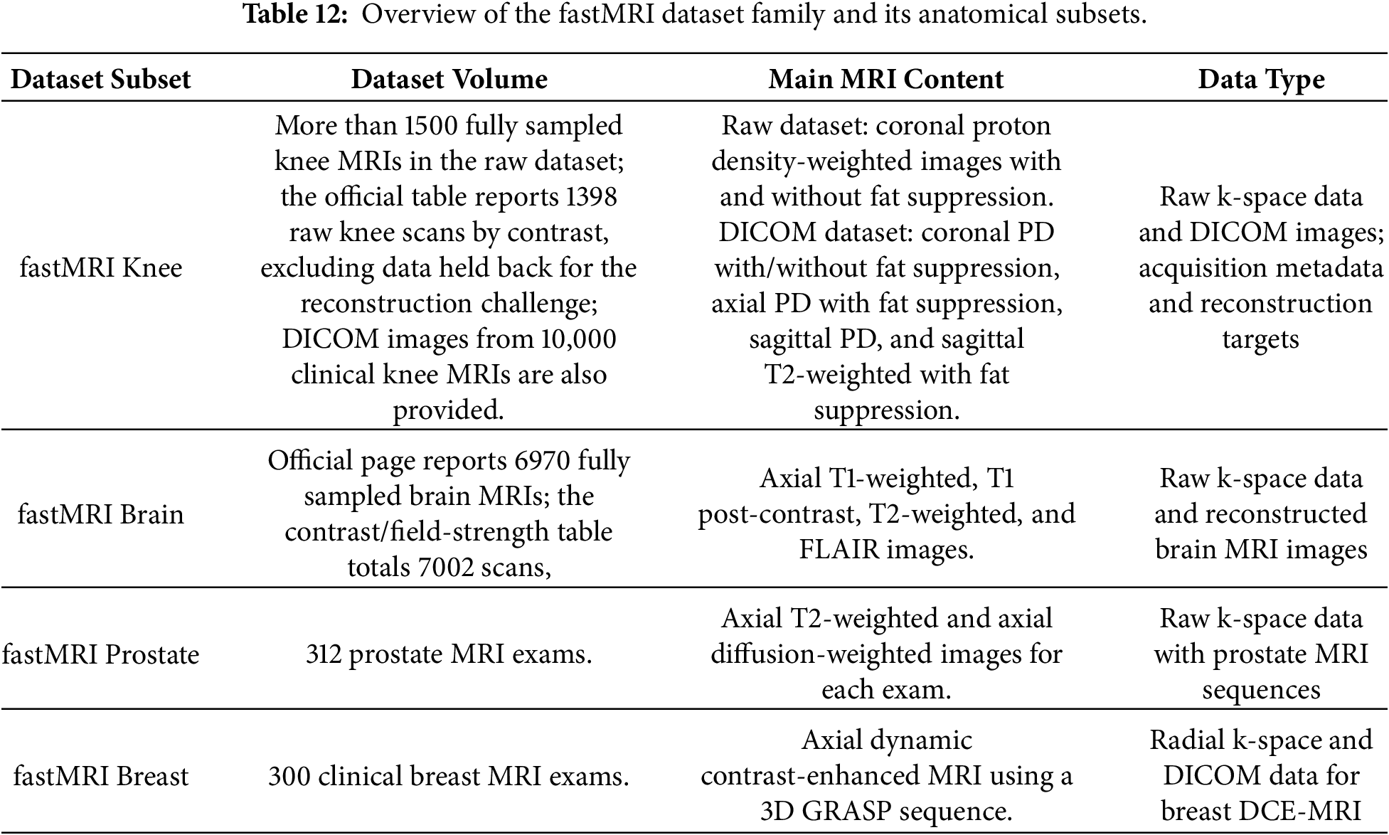
fastMRI has particular methodological value because it links MRI acquisition physics with deep learning-based image recovery. Models trained on fastMRI data often need to account for k-space measurements, coil sensitivity, undersampling patterns, and the relationship between frequency-domain data and image-domain reconstruction. In this sense, fastMRI is not only a benchmark for accelerated MRI reconstruction, but also a resource that may support later-stage applications, including segmentation, diagnosis, and quantitative image analysis.

3.8 Comparative Summary of Dataset Roles

The dataset families reviewed in this section indicate that public 3D MRI resources do not function as a single uniform benchmark. Instead, they define different research settings according to anatomy, disease context, imaging protocol, and annotation type. Brain tumor and stroke datasets, including BraTS, MSD Brain Tumor, and ATLAS, primarily support lesion or tumor delineation because they provide spatial annotations. ADNI, OASIS, and MIRIAD are more similar to clinical cohort resources, where structural MRI is linked with diagnosis, cognitive measures, biomarkers, and longitudinal follow-up. IXI and HCP are commonly used as reference datasets for anatomical representation, preprocessing validation, and methodological testing. OAI expands the reviewed literature into musculoskeletal imaging, whereas fastMRI shifts attention toward MRI acquisition, reconstruction, and image-quality enhancement.

These differences also affect how experimental results should be interpreted. Performance on BraTS or ATLAS mainly reflects the ability to segment tumors or lesions, whereas ADNI- or OASIS-based studies usually assess subject-level classification, disease staging, or progression prediction. IXI and HCP can support anatomical modeling, reconstruction, or preprocessing studies, but results obtained on these datasets should not be read as direct evidence of clinical diagnostic validity. Taken together, the dataset family determines the anatomical scope, supervision type, and appropriate evaluation strategy of a 3D MRI-based computer vision study. The next section therefore turns to the question of how volumetric MRI data are organized before model training, including 2D slices, 2.5D inputs, full 3D volumes, and multi-view representations.

4  Input Paradigms for 3D MRI-Based Computer Vision

4.1 Overview of Volumetric MRI Input Organization

A 3D MRI scan contains anatomical and intensity information across three spatial dimensions, but it does not have to be processed as a complete volume. In practice, the input format is shaped by voxel spacing, slice thickness, field of view, acquisition plane, imaging sequence, anatomical target, annotation type, and available computational resources [71,72]. For this reason, studies using the same dataset or addressing a similar task may still adopt different ways of organizing the MRI volume before model training.

The main input paradigms include 2D slice-based input, 2.5D adjacent-slice input, full 3D or patch-based input, and multi-view input. A 2D strategy is computationally efficient and compatible with mature 2D architectures, although it offers only limited inter-slice context. A 2.5D design introduces nearby slices to provide partial volumetric information while keeping the computational cost closer to 2D processing. Full 3D and patch-based strategies preserve spatial continuity more directly, making them well suited to tasks that depend on volumetric structure, such as segmentation and reconstruction, but they usually require more memory and more careful preprocessing. Multi-view strategies use axial, coronal, and sagittal planes to capture complementary anatomical information without relying entirely on dense 3D computation.

Fig. 10 summarizes these input organizations. These paradigms are discussed in more detail in the following subsections, with attention to their advantages, limitations, and task suitability.

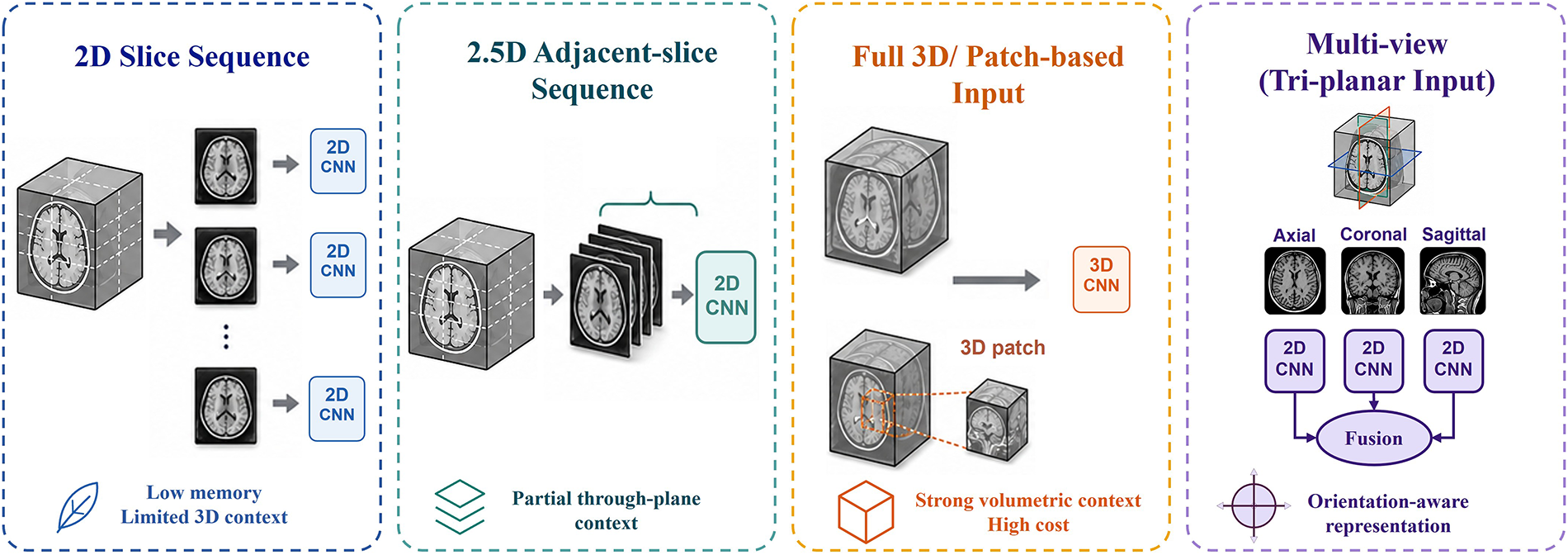
Figure 10: Schematic illustration of major input paradigms for 3D MRI-based computer vision.

4.2 Structural Computational Complexity across Input Paradigms

Computational cost is an important factor in selecting an input paradigm. FLOPs, parameter count, peak GPU memory, and inference time are jointly influenced by input size, network depth and width, batch size, numerical precision, patch configuration, fusion strategy, software implementation, and hardware platform. Therefore, this section focuses on the structural computational scaling of representative paradigm implementations rather than assigning universal numerical values to each paradigm.

For a standard 2D convolution with an output feature map of size Ho×Wo, Cin input channels, Cout output channels, and a kernel of size kh×kw, the approximate number of multiply–accumulate operations is 𝒞2D≈HoWoCinCoutkhkw. The corresponding parameter count is approximately 𝒫2D≈CinCoutkhkw [73].

A 3D convolution introduces an additional depth dimension. For an output volume of size Do×Ho×Wo and a kernel of size kd×kh×kw, the approximate operation count becomes 𝒞3D≈DoHoWoCinCoutkdkhkw, with a parameter count of 𝒫3D≈CinCoutkdkhkw [74].

The computational difference between 2D and 3D models therefore arises from both the additional kernel dimension and the volumetric size of intermediate feature maps [75,76].

The complexity of 2.5D methods depends on how through-plane information is incorporated. In a simple adjacent-slice stacking design, m neighboring slices are treated as input channels. If the subsequent 2D backbone remains unchanged, the main computational increase occurs in the first convolutional layer, where the input-channel dimension increases from Cin to approximately mCin. The remaining layers continue to use 2D operations. This form of 2.5D processing is therefore computationally closer to a 2D network than to a full 3D network [77].

By contrast, 2.5D methods that encode slices independently and subsequently apply recurrent, attention-based, Transformer-based, or other feature-fusion modules have a different cost structure. Their approximate computation can be expressed conceptually as 𝒞2.5D≈m𝒞encoder+𝒞fusion, where m is the number of processed slices. These methods may require repeated slice encoding and additional memory for retaining multiple feature representations. Consequently, the computational demand of 2.5D methods cannot be summarized by a single fixed value [78].

Multi-view methods usually process V anatomical planes, most commonly the axial, coronal, and sagittal views. Their overall computation can be approximated as 𝒞MV≈V𝒞2D+𝒞fusion.

If view-specific branches use independent parameters, the total parameter count may increase approximately with the number of views. If weights are shared, parameter growth is limited, although each view still requires a separate forward pass. Decision-level fusion introduces relatively little additional computation, whereas feature-level fusion may require multiple intermediate feature maps to be retained simultaneously and therefore increases both computation and memory demand [79,80].

Table 13 summarizes these paradigm-level structural differences. The comparison describes general computational tendencies rather than fixed numerical benchmarks.

4.3 2D Slice-Based Input

In the 2D slice-based paradigm, a 3D MRI volume is decomposed into individual slices or ordered slice sequences, which are then processed by 2D CNNs [81–84]. This strategy reduces GPU memory demand, supports larger batch sizes, and allows the use of mature 2D architectures. However, it weakens inter-slice continuity and may introduce inconsistency between slice-level predictions and subject-level labels.

In some representative studies, Gautam and Singh [85] used T1-weighted 3D MRI from ADNI for Alzheimer’s disease classification. Their pipeline converted each 3D volume into 2D slices and adapted pretrained 2D CNNs, including VGG16, MobileNet, DenseNet121, and NASNetMobile. Their study shows how 2D slicing enables the reuse of pretrained image-classification backbones for volumetric MRI.

Alirr [86] applied a 2D U-Net-based design to ischemic stroke lesion segmentation using multimodal MRI, including DWI, ADC, and FLAIR. The study emphasized the practical advantage of lightweight 2D models, especially when full 3D networks require high memory and may overfit under limited annotations.

Ahanger et al. [87] proposed AlzhiNet for Alzheimer’s disease classification using 3D volumetric MRI and a self-attention mechanism. Although the input data were volumetric, the model emphasized slice-level contribution to diagnostic decisions, showing that 2D or slice-aware representations can improve interpretability in subject-level diagnosis.

Li et al. [88] extended the role of 2D input to MRI reconstruction. Their parallel dual-domain crossing network used image-domain and k-space-domain representations with multimodal feature fusion. This example indicates that 2D input in 3D MRI studies is not limited to slice classification, but can also serve as the computational unit for image recovery.

2D slice-based input is useful when computational efficiency, pretrained 2D architectures, or slice-level interpretability is prioritized. Its main limitation remains the reduced ability to represent three-dimensional spatial continuity. Table 14 summarizes representative studies that explicitly reported 3D-to-2D conversion.

4.4 2.5D Slice-Based Input

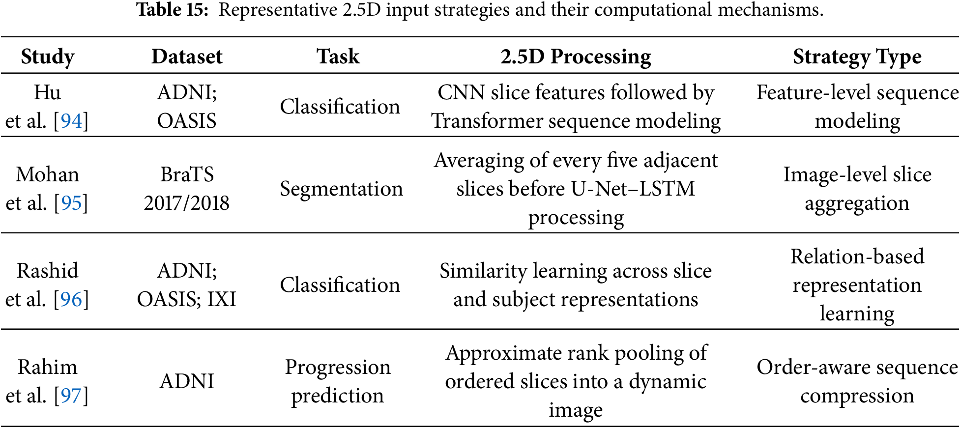
The 2.5D slice-based input paradigm is used here as a representation-level category rather than as a single computational mechanism [89–93]. It includes methods that introduce inter-slice or through-plane information while avoiding direct full-volume processing with 3D operations. Depending on where and how this information is incorporated, the reviewed studies can be distinguished as image-level adjacent-slice aggregation, feature-level slice-sequence modeling, relation-based inter-slice representation learning, and order-aware sequence compression. These strategies differ substantially in their computational operations and in the amount of volumetric information they preserve, although all occupy an intermediate position between independent 2D slice processing and full 3D modeling.

Conv-Swinformer [94] represents a feature-level slice-sequence modeling strategy for Alzheimer’s disease classification using ADNI and OASIS. A CNN first extracts planar features from individual slices, after which a Transformer encoder models semantic dependencies across the ordered slice sequence. Inter-slice information is therefore introduced after slice-level feature extraction rather than through direct aggregation of the original MRI slices. This strategy preserves sequence-level relationships while maintaining predominantly 2D feature extraction.

Mohan et al. [95] adopted an image-level adjacent-slice aggregation strategy for brain tumor segmentation using BraTS 2017 and BraTS 2018. Every five neighboring slices were averaged, reducing the original sequence of 155 slices to 31 aggregated images, followed by tumor-oriented region cropping and U-Net–LSTM segmentation. Unlike feature-level sequence modeling, this method introduces through-plane context before feature extraction. Its averaging operation reduces computational cost but may also suppress fine inter-slice variation.

Biceph-Net [96] represents a relation-based inter-slice learning strategy. The method processes 2D slices extracted from 3D MRI volumes and uses deep similarity learning to constrain intra-slice and inter-slice representations. Rather than explicitly stacking or averaging adjacent slices, it preserves subject-level relationships in the learned embedding space. Its use of volumetric context is therefore relational rather than based on direct image-level fusion.

Rahim et al. [97] used an order-aware sequence-compression strategy for Alzheimer’s disease progression detection. Approximate rank pooling was applied to an ordered sequence of MRI slices to generate a single dynamic 2D image for each volume and time point. The resulting image encodes part of the slice-order information but compresses the original sequence into one representation. This differs from both adjacent-slice aggregation and explicit sequence modeling because inter-slice information is summarized before CNN–BiLSTM analysis.

Table 15 summarizes these representative strategies. In this review, 2.5D does not denote a uniform network architecture or fusion mechanism. It denotes a family of representations that use partial volumetric information without directly applying full 3D processing to the original MRI volume. Although these studies are grouped under the 2.5D input paradigm, they do not employ the same computational mechanism. They can be distinguished as feature-level sequence modeling, image-level slice aggregation, relation-based representation learning, and order-aware sequence compression, according to where and how inter-slice information is introduced.

However, 2.5D methods still provide less complete spatial context than full 3D models, and different implementations are not directly comparable unless the conversion process is clearly described. Therefore, studies should report how neighboring slices or slice sequences are constructed, whether information is compressed or averaged, and whether all derived samples from the same subject are split consistently.

4.5 Full 3D Volume and Patch-Based Input

Full 3D volume input provides the most direct way to represent volumetric MRI in deep learning models. It retains spatial information across all three anatomical dimensions and is therefore well matched to tasks that depend on volumetric structure [98–101]. In multimodal MRI settings, different sequences are commonly stacked as separate input channels, allowing 3D networks to learn inter-slice continuity, spatial relationships, and lesion morphology within a unified volumetric representation.

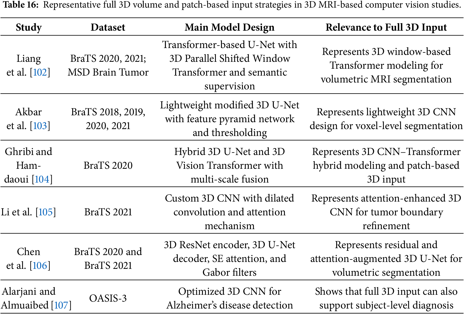
Liang et al. [102] developed 3D PSwinBTS for multimodal brain tumor segmentation, arguing that slice-based processing can discard important volumetric information. This 3D shifted-window Transformer module was designed to capture contextual information along multiple axes while controlling computational cost. Akbar et al. [103] introduced Yaru3DFPN, a lightweight 3D U-Net variant combined with feature pyramid networks. By using 3D operations, the model can represent voxel connectedness across neighboring slices.

Hybrid CNN–Transformer designs further show how full 3D input can be adapted to balance local detail and broader spatial dependency. Ghribi and Hamdaoui [104] combined a 3D U-Net with a 3D Vision Transformer for multimodal brain tumor segmentation. In this framework, 3D CNN components capture local anatomical features, whereas transformer modules model longer-range spatial relationships. The use of a patch-based pipeline also shows that full 3D modeling does not always require processing the entire MRI volume at once; local volumetric patches can serve as the effective input unit.

Other studies have focused on improving boundary representation, feature selectivity, and texture-aware volumetric segmentation within 3D networks. Li et al. [105] proposed Arouse-Net, a 3D CNN for glioblastoma segmentation in multi-parametric MRI. Its use of dilated convolutions and attention mechanisms expanded the receptive field and emphasized tumor boundary information. Chen et al. [106] developed dSEAT-UNet for multimodal brain tumor segmentation by integrating residual encoding, squeeze-and-excitation (SE) attention, and Gabor filtering into a 3D U-Net framework, with the aim of strengthening both local–global feature extraction and texture-sensitive segmentation.

Although segmentation is the most common setting for full 3D input, volumetric modeling can also support subject-level diagnosis. Alarjani and Almuaibed [107] applied a 3D CNN to Alzheimer’s disease detection using OASIS-3 MRI. Unlike slice-based classification methods, their model processed 3D MRI scans directly to preserve whole-brain spatial information. This example indicates that full 3D input may be useful beyond dense prediction tasks when the diagnostic target depends on distributed anatomical patterns or global volumetric context.

Table 16 summarizes representative full 3D and patch-based input strategies. These examples indicate that full 3D input provides the most direct representation of volumetric MRI. It preserves inter-slice continuity, supports voxel-level prediction, and enables models to learn 3D shape, boundary, volume, and spatial-location patterns. This makes it particularly suitable for segmentation and other tasks requiring dense anatomical reasoning.

The main cost of this paradigm is computational complexity. Full-volume 3D CNNs or 3D Transformers require substantially more GPU memory than 2D methods, especially for high-resolution or multimodal MRI.

4.6 Multi-View and Tri-Planar Input

Multi-view or tri-planar input organizes 3D MRI by extracting 2D views from multiple anatomical planes, usually axial, coronal, and sagittal [108–110]. These views can be processed by separate networks, shared branches, transformer modules, or ensemble models, and then fused at the feature or decision level [111–113]. Compared with single-plane 2D input, this strategy provides broader anatomical coverage; compared with full 3D input, it usually requires lower computational cost.

Mossa and Çevik [114] proposed a multiview CNN ensemble framework for overall survival prediction in brain tumor patients using multimodal MRI. Their method represented 3D MRI as axial, sagittal, and coronal slice sets, trained plane-specific CNN models, and fused predicted probabilities with machine-learning algorithms. This example shows a typical multi-view design based on 2D CNNs and ensemble fusion.

Alp et al. [115] used multi-plane MRI slices for Alzheimer’s disease classification based on ADNI T1-weighted MRI. The standardized 3D volumes were split into axial, coronal, and sagittal slices, and transformer-based models were used to extract slice-level features and model slice-sequence dependencies. This study illustrates how multi-view input can be combined with Vision Transformer and sequence modeling.

Rahim et al. [116] proposed a more explicit multi-view framework for detecting progression from stable MCI to progressive MCI or AD. Their method used axial, coronal, and sagittal views simultaneously, extracted plane-specific features with CNN backbones, refined them with attention modules, and combined them through ensemble strategies. The use of gradient-weighted class activation mapping (Grad-CAM) further showed how different views contributed to the final prediction.

Islam et al. [117] applied a multi-plane slice representation to Alzheimer’s disease detection using OASIS-2 structural MRI. Their preprocessing framework extracted evenly distributed 2D slices from the axial, coronal, and sagittal planes and constructed both plane-specific datasets and a combined three-plane dataset. The resulting slices were processed by a lightweight hybrid classical–quantum convolutional neural network, in which a 2D CNN extracted image features before a parameterized quantum circuit performed binary classification. Unlike multi-branch architectures that fuse view-specific features or predictions, this study combined slices from the three anatomical planes at the dataset level.

Table 17 summarizes representative multi-view and tri-planar input strategies. This paradigm offers a practical balance between 2D efficiency and 3D anatomical coverage. Its performance depends on slice selection, view-fusion strategy, and subject-level data splitting.

4.7 Summary and Transition to Downstream Tasks

The preceding subsections show that 3D MRI can be represented in multiple forms before model training. Each represents a different balance among spatial-context preservation, computational demand, preprocessing sensitivity, data availability, and task requirements. As summarized in Table 18, 2D methods offer low peak memory and straightforward use of pretrained models, but their slice-wise processing may weaken through-plane consistency. 2.5D methods introduce limited inter-slice context while retaining much of the efficiency of 2D processing, although their effectiveness depends strongly on slice selection and fusion design. Full 3D methods provide the most direct representation of volumetric anatomy, but require greater activation memory and are more sensitive to voxel spacing, resampling, spatial normalization, multimodal registration, and volume size. Multi-view methods combine complementary anatomical planes without relying entirely on volumetric convolution, but their effectiveness depends on consistent plane extraction and alignment across views and modalities.

These trade-offs also explain why input-paradigm selection differs across downstream tasks. Classification and diagnosis can often tolerate compressed or view-based representations when subject-level cues are distributed across the volume. Segmentation and reconstruction generally benefit more directly from spatial continuity and local volumetric structure, whereas super-resolution may use 2D, multi-slice, 2.5D, or full 3D designs depending on whether the target is primarily in-plane enhancement or through-plane recovery. The following section therefore examines downstream tasks in relation to their output requirements.

5  Downstream Tasks in 3D MRI-Based Computer Vision

After reviewing datasets and input paradigms, this section focuses on the main computer vision tasks supported by 3D MRI. These tasks are shaped by the available labels and expected outputs. This distinction affects how models are designed and evaluated. Classification and diagnosis tasks usually aggregate information from slices, views, modalities, or volumes into a subject-level prediction. Segmentation requires spatially precise voxel-level output, making anatomical continuity and localization more important. Reconstruction and restoration recover images from degraded or undersampled data, while super-resolution aims to generate high-resolution MRI from low-resolution input.

This section is organized to emphasize the diversity of dataset–task–input paradigm configurations rather than to rank paradigms using pooled performance values. Reported metrics are affected by differences in dataset versions, target definitions, preprocessing, model architectures, data splits, and evaluation protocols, making direct cross-study averaging potentially misleading. The task-oriented presentation therefore helps readers identify relevant datasets and input paradigms before consulting the original studies for detailed performance results within their specific experimental contexts.

5.1 Detection, Diagnosis, and Classification

5.1.1 Task Definition and Evaluation Metrics

Detection, diagnosis, and classification are common tasks in 3D MRI-based computer vision. They assign binary, categorical, ordinal, or region-specific labels to MRI-derived inputs, depending on the clinical question and annotation type [118–122]. The prediction target may be defined at the subject level, scan level, anatomical-region level, or lesion level. Although these tasks are often discussed together, their output granularity differs. Diagnosis and classification usually produce subject-level or scan-level labels. Detection may also produce categorical results, but it often focuses on whether an abnormality exists in a specific anatomical region. In this sense, detection lies between general classification and precise localization.

In this task family, the relationship between the input unit and the prediction unit is central. A subject-level label may be assigned to an entire MRI examination, whereas the model input may consist of multiple paradigms. This creates a methodological gap between the imaging representation and the clinical label. Therefore, classification performance is not determined only by the classifier architecture; it is also shaped by how MRI information is sampled, aggregated, fused, and linked to the reference label [123–127].

Evaluation for detection, diagnosis, and classification tasks is usually based on the agreement between predicted and reference labels. Let TP, TN, FP, and FN denote true positives, true negatives, false positives, and false negatives, respectively. Common metrics include accuracy, sensitivity, specificity, precision, and F1-score, as shown in Eqs. (1)–(5):

Accuracy=TP+TNTP+TN+FP+FN(1)

Sensitivity=Recall=TPTP+FN(2)

Specificity=TNTN+FP(3)

Precision=TPTP+FP(4)

F1=2×Precision×RecallPrecision+Recall(5)

Accuracy measures the overall proportion of correct predictions. Sensitivity measures the ability to detect positive cases and is especially important for screening-oriented tasks, whereas specificity measures the ability to correctly identify negative cases. Precision reflects the reliability of positive predictions, and F1-score balances precision and recall. These metrics are frequently used in medical image classification and diagnostic accuracy studies [128].

For probabilistic classifiers, the receiver operating characteristic curve plots the true positive rate against the false positive rate across decision thresholds. The area under the curve is commonly defined as Eq. (6):

AUC=∫01TPR(FPR)dFPR(6)

where TPR is the true positive rate and FPR is the false positive rate. AUC is widely used in medical image classification because it evaluates discrimination across thresholds, but it should not be interpreted alone when class imbalance, calibration, or clinical decision thresholds are important [129].

The metrics above represent the main evaluation measures used for classification-oriented tasks in this review.

5.1.2 Representative Studies and Methodological Interpretation

Alzheimer’s disease classification is a typical subject-level diagnosis task using volumetric brain MRI. Rehman et al. [130] introduced 3D-MobiBrainNet for multi-class classification on ADNI 3D MRI. By integrating axial, coronal, and sagittal information, the method distinguishes cognitively normal, mild cognitive impairment, and Alzheimer’s disease groups, illustrating how multi-plane input can support subject-level diagnostic prediction.

Brain tumor classification involves a different form of input aggregation, where multimodal MRI sequences are combined at the patient level. Montaha et al. [131] used a TimeDistributed-CNN-LSTM framework for glioma grading with BraTS MRI. The four standard modalities, T1, T1ce, T2, and FLAIR, were treated as complementary patient-level inputs for distinguishing high-grade and low-grade gliomas. This setting highlights the diagnostic value of integrating sequence-specific information in tumor-related classification.

In musculoskeletal MRI, detection tasks may combine categorical prediction with anatomical localization. Tack et al. [132] developed a multi-task deep learning method for meniscal tear detection using OAI knee MRI. The model predicts tears in specific meniscal subregions and incorporates bounding-box regression, indicating that classification-oriented outputs can be extended with region-aware localization.

Knee osteoarthritis detection further shows how large clinical cohorts and incomplete supervision can shape model design. Berrimi et al. [133] designed a semi-supervised multi-view MRI framework using OAI data. By combining labeled and unlabeled MRI scans, the method examines the contribution of different views to osteoarthritis detection and addresses the partially labeled nature of clinical imaging datasets.

A related study by Berrimi et al. [134] introduced M3NET for multi-view, multimodal, and multi-task knee injury classification, also using OAI data. The framework combines 3D MRI views with 2D X-ray images and jointly evaluates cartilage and meniscus damage. This design is closer to realistic diagnostic practice, where multiple imaging views, complementary modalities, and related tissue abnormalities are considered together.

Table 19 summarizes these representative studies in terms of dataset source, prediction level, input paradigm, and evaluation metrics, rather than detailed network architecture.

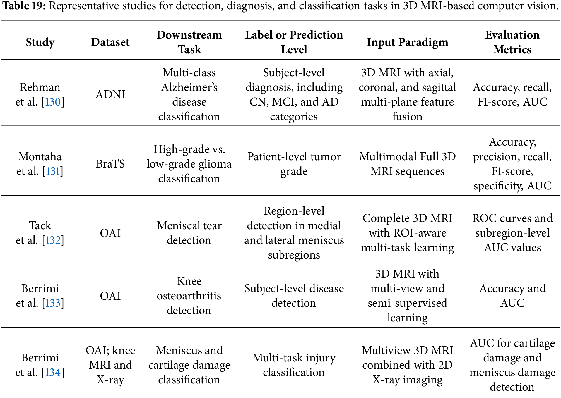
Overall, detection, diagnosis, and classification tasks provide a broad testbed for 3D MRI-based computer vision. Their methodological diversity reflects the diversity of clinical questions and dataset structures. Rather than treating the classifier architecture as the main object of comparison, these studies are best understood by examining how the available MRI data are organized into inputs, how those inputs are linked to clinically meaningful prediction targets, and how evaluation metrics reflect the intended unit of clinical decision-making.

5.2 Segmentation and Lesion Delineation

5.2.1 Task Definition and Evaluation Metrics

Segmentation and lesion delineation aim to assign a label to each pixel or voxel. The output is therefore a spatial mask that delineates anatomical structures, lesions, tumors, or pathological subregions [135–139]. The input paradigm is particularly important in segmentation. 2D slice-based models are computationally efficient and can increase the number of training samples by decomposing 3D volumes into slices, but they may lose inter-slice continuity. Full 3D models preserve volumetric context and lesion morphology more directly, but they require more GPU memory and are sensitive to dataset size, patch sampling, and preprocessing. Multimodal MRI further adds another layer of complexity because different sequences may highlight different tissue characteristics. Thus, segmentation studies should be interpreted through the relationship among annotation type, input organization, anatomical target, and evaluation unit [140–144].

Segmentation performance is commonly assessed using overlap-based and boundary-based metrics. Recent discussions on medical image segmentation evaluation emphasize that no single metric fully captures segmentation quality, and that overlap metrics such as Dice and Jaccard should be interpreted together with boundary-distance metrics such as Hausdorff distance or average surface distance when contour accuracy is clinically important [145,146].

Let P denote the predicted segmentation mask and G denote the ground-truth mask. The Dice similarity coefficient, also called Dice score or DSC, is one of the most widely used metrics in medical image segmentation as shown in Eq. (7):

Dice=DSC=2∣P∩G∣∣P∣+∣G∣(7)

Dice measures the spatial overlap between the predicted and reference masks. A higher Dice score indicates better regional agreement.

Another common overlap metric is Intersection over Union, also known as the Jaccard index, as shown in Eq. (8):

IoU=Jaccard=∣P∩G∣∣P∪G∣(8)

IoU also measures the agreement between prediction and ground truth, but it uses the union of the two masks as the denominator. Dice and IoU are mathematically related, but Dice is more frequently reported in many medical image segmentation benchmarks.

For lesion-level segmentation, previously defined classification metrics such as precision, recall, and F1-score can also be applied at the lesion level rather than the voxel level. This is useful when the number of correctly detected lesions matters, especially for small or multiple lesions [147].

Boundary-based metrics are also important because high overlap does not always imply accurate contour delineation. The Hausdorff distance measures the largest boundary discrepancy between the predicted and reference masks, as Eq. (9):

HD(P,G)=max{supp∈∂Pinfg∈∂Gd(p,g),supg∈∂Ginfp∈∂Pd(g,p)}(9)

where ∂P and ∂G denote the boundaries of the predicted and ground-truth masks, and d(p,g) is the distance between boundary points. Since the standard Hausdorff distance is sensitive to outliers, many medical segmentation studies report the 95th percentile Hausdorff distance, as Eq. (10):

HD95=percentile95(d(∂P,∂G))(10)

Average surface distance (ASD) is another boundary-related metric, as Eq. (11):

ASD(P,G)=1∣∂P∣+∣∂G∣(∑p∈∂Pming∈∂Gd(p,g)+∑g∈∂Gminp∈∂Pd(g,p))(11)

ASD reflects the average boundary mismatch between the predicted and reference surfaces. In general, Dice and IoU evaluate regional overlap, whereas HD95 and ASD evaluate boundary accuracy.

Therefore, segmentation studies should report metrics that match the clinical objective: overlap metrics are useful for estimating lesion or structure extent, while boundary metrics are important for tasks requiring accurate contour delineation, such as tumor margin assessment, surgical planning, or radiotherapy planning [148–150]. The interpretation of these metrics also depends on the input paradigm and the dimensional level at which predictions are evaluated. A 2D slice-based model may achieve favorable Dice or IoU scores on individual slices while producing discontinuous, jagged, or anatomically implausible boundaries after the slices are reassembled into a three-dimensional volume. Such through-plane inconsistencies may be insufficiently reflected by overlap-based metrics but can lead to larger HD95 or ASD values during volume-level evaluation.

A 2.5D model incorporates limited neighboring-slice context and may improve through-plane consistency relative to independent 2D processing, although its measured performance depends on the number and spacing of adjacent slices and on the fusion strategy. Multi-view methods may reduce orientation-specific errors by combining information from different anatomical planes, but prediction fusion and interpolation can smooth small structures or introduce disagreement among views. Full 3D models directly optimize volumetric predictions and are generally better positioned to preserve spatial continuity, although their overlap and boundary metrics remain sensitive to voxel anisotropy, resampling, patch aggregation, and post-processing.

Consequently, comparisons among input paradigms should not rely on Dice alone. Studies should report whether evaluation is performed per slice or per volume, specify voxel spacing and resampling procedures, and combine overlap-based metrics with boundary-distance measures when volumetric continuity and contour accuracy are clinically relevant.

5.2.2 Representative Studies and Methodological Interpretation

Brain tumor segmentation based on BraTS is one of the most common settings in 3D MRI segmentation. Pedada et al. [151] proposed a modified U-Net for tumor segmentation using BraTS 2017 and BraTS 2018. The study evaluated tumor regions such as whole tumor, tumor core, and enhancing core, representing a typical 2D or slice-based U-Net-style segmentation approach. It also reflects a common trade-off: 2D methods are easier to train and less memory-intensive, but may capture less volumetric context than 3D models.

Xing et al. [152] proposed a 3D Dual Encoder Mirror Difference ResU-Net for multimodal brain tumor segmentation using BraTS 2018 and BraTS 2019. The model used T1, T1ce, T2, and FLAIR images and processed volumetric information with a full 3D design. This study represents a 3D multimodal segmentation paradigm, where spatial continuity and complementary MRI sequences are used to delineate tumor subregions.

Di Matteo et al. [153] studied sub-acute and chronic stroke lesion segmentation using ATLAS v2.0 and an independent clinical cohort. The work compared T1-only fine-tuning with T1 + FLAIR multimodal fusion strategies, and the best results were obtained with a late-fusion ensemble. This example extends segmentation analysis from tumor benchmarks to stroke lesions, clinical transferability, multimodal fusion, and lesion-volume variability.

Yeoh et al. [154] investigated knee MRI segmentation and osteoarthritis diagnosis using OAI data. Their 3D multi-task model jointly performed knee structure segmentation and OA classification, showing that segmentation can serve both as an independent anatomical analysis task and as support for downstream diagnosis. This example also illustrates the role of structure segmentation in musculoskeletal MRI.

Table 20 summarizes these representative segmentation studies according to dataset source, segmentation target, input paradigm, supervision type, and evaluation metrics.

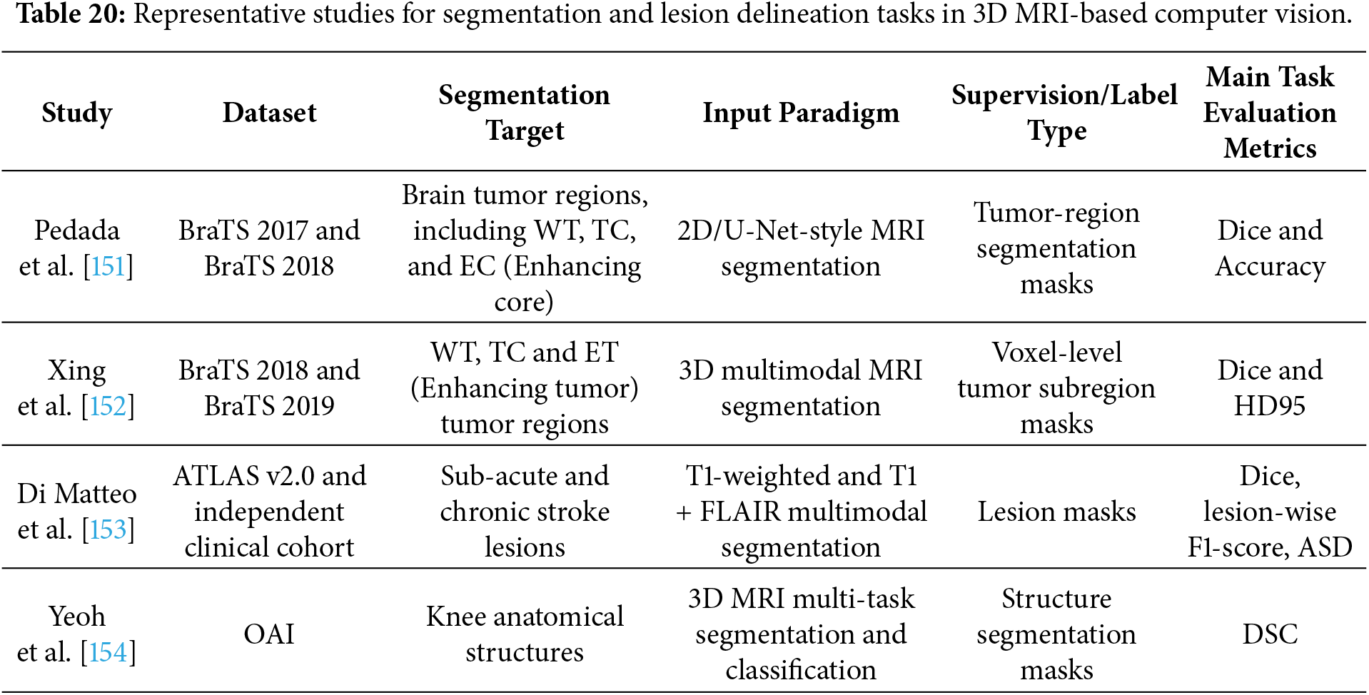
Overall, segmentation and lesion delineation tasks require evaluation at the voxel, lesion, surface, or anatomical-structure level. Dice and IoU summarize regional overlap, lesion-wise F1-score reflects lesion detection consistency, and HD95 or ASD evaluates boundary accuracy. Therefore, segmentation studies should clearly report the segmentation target, annotation source, input dimensionality, modality combination, evaluation metric, and whether evaluation is performed per slice, per volume, per lesion, or per anatomical structure.

5.3 Reconstruction and Image Restoration

5.3.1 Task Definition and Evaluation Metrics

Reconstruction and image restoration aim to recover high-quality MRI images or volumes from undersampled, incomplete, noisy, corrupted, or artifact-contaminated data. In accelerated MRI, the input is often undersampled k-space data or zero-filled reconstructions, and the target is a fully sampled or clinically acceptable reference image. In image restoration, the input may be degraded by noise, motion artifacts, intensity inhomogeneity, aliasing, or missing information. These tasks are therefore closely related to MRI acquisition and image-quality enhancement, and are commonly evaluated on datasets such as fastMRI, IXI, and other structural MRI resources [155–158].

Let X denote the reference image or volume and X^ denote the reconstructed or restored output. Common evaluation metrics include voxel-wise error metrics, signal-fidelity metrics, and structural-similarity metrics. Mean squared error (MSE), root mean squared error (RMSE), and mean absolute error (MAE) are basic measures of reconstruction error, as shown in Eqs. (12)–(14):

MSE=1N∑i=1N(Xi−X^i)2(12)

RMSE=1N∑i=1N(Xi−X^i)2(13)

MAE=1N∑i=1N∣Xi−X^i∣(14)

where N denotes the number of pixels or voxels. These metrics quantify global intensity differences between the reconstructed image and the reference image. Lower values indicate smaller reconstruction errors.

Normalized mean squared error (NMSE) is widely used in MRI reconstruction benchmarks because it normalizes the squared error by the energy of the reference image, as Eq. (15):

NMSE=∥X−X^∥22∥X∥22(15)

Peak signal-to-noise ratio (PSNR) is another common metric for signal fidelity, as Eq. (16):

PSNR=10log10⁡(MAXX2MSE)(16)

where MAXX is the maximum possible or normalized image intensity. Higher PSNR usually indicates better reconstruction quality.

Structural similarity index measure (SSIM) is frequently reported to assess whether the reconstructed image preserves local structural information, as Eq. (17):

SSIM(X,X^)=(2μXμX^+C1)(2σXX^+C2)(μX2+μX^2+C1)(σX2+σX^2+C2)(17)

where μ, σ2 and σXX^ denote local mean, variance, and covariance, respectively, and C1 and C2 are stability constants. Compared with MSE or PSNR, SSIM better reflects local contrast and structural similarity and is therefore commonly used in MRI reconstruction and restoration studies.

Reconstruction and restoration performance is commonly evaluated using error-based metrics, such as MSE, NMSE, MAE, and RMSE, together with image-quality metrics, such as PSNR and SSIM, as well as visual assessment. However, high quantitative scores do not necessarily guarantee diagnostic reliability. Reconstructed images may still lose subtle lesions, smooth anatomical boundaries, or introduce visually plausible but clinically incorrect details.

5.3.2 Representative Reconstruction and Image Restoration Methods

Recent 3D MRI reconstruction and image restoration studies mainly address accelerated reconstruction from undersampled k-space data, model-based deep reconstruction, dual-domain learning, and image-domain restoration. Compared with diagnosis or segmentation, these tasks are more closely linked to the MRI acquisition process. As a result, many methods combine deep learning with Fourier-domain constraints, data consistency terms, tensor priors, or multimodal image information.

FAS-Net, introduced by Liu et al. [159], is representative of accelerated high-resolution MRI reconstruction. The method uses faster Fourier convolution to enlarge the receptive field and reduce global artifacts, while a split-slice strategy is adopted to lower the memory burden during high-resolution 3D reconstruction. Experiments on NYU fastMRI and Stanford MRI Data demonstrated its applicability to high-resolution multi-coil 3D MRI reconstruction, making it a practical example of volumetric reconstruction under memory constraints.

PALADIN, developed by Wu et al. [160], illustrates a model-based deep reconstruction strategy for 3D CS (compressed sensing)-MRI. The framework combines tensor low-rank priors, data fidelity, CNN-based denoising, and learned reconstruction modules within an optimization-based formulation. Rather than treating the neural network as a purely black-box predictor, this design embeds deep learning components into an inverse-problem framework with interpretable reconstruction constraints.

Safari et al. [161] proposed SSAD-MRI, a self-supervised adversarial diffusion model for fast MRI reconstruction. Unlike supervised reconstruction methods that depend on fully sampled reference data, SSAD-MRI reconstructs images from undersampled k-space without requiring fully sampled targets during training. By combining self-supervised data consistency with diffusion-based reconstruction, the method reduces reliance on fully sampled datasets and improves robustness under high acceleration and domain-shift settings.

AMC-Net, proposed by Li et al. [88], represents a dual-domain reconstruction approach. The model processes k-space and image-domain information in parallel and enables interaction between the two branches. Its multimodal feature-fusion design further suggests that reconstruction can benefit not only from physical-domain correspondence, but also from structural information provided by related MRI modalities.

Table 21 summarizes these representative reconstruction and restoration studies according to dataset source, reconstruction target, input paradigm, main methodological design, and evaluation metrics. Unlike classification and segmentation, reconstruction outputs are still images or volumes rather than labels or masks.

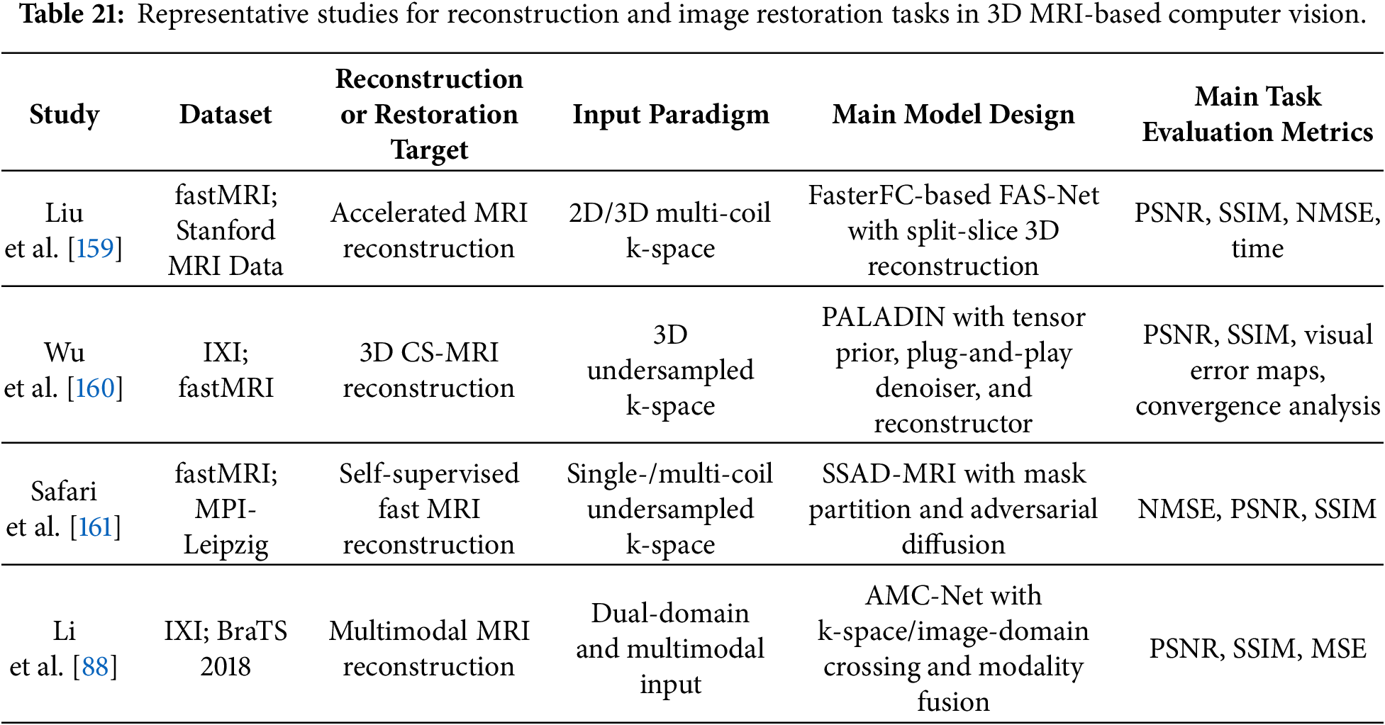
Overall, these studies suggest that current MRI reconstruction research is moving toward frameworks that combine k-space consistency, volumetric or cross-slice information, learned priors, multimodal cues, and self-supervised training strategies.

5.4 Super-Resolution

5.4.1 Task Definition and Evaluation Metrics

Super-resolution is an image enhancement task that aims to reconstruct high-resolution MRI images or volumes from low-resolution inputs. In 3D MRI analysis, this task is particularly important because high spatial resolution is usually associated with longer acquisition time, lower signal-to-noise ratio, greater sensitivity to patient motion, and higher imaging cost. Therefore, MRI super-resolution provides a computational strategy for improving apparent spatial resolution without directly increasing scanning burden [162–165].

Let XLR denote the low-resolution MRI input and XHR denote the corresponding high-resolution reference image or volume. A super-resolution model learns a mapping function fθ to generate a super-resolved output XSR, as shown in Eq. (18):

XSR=fθ(XLR)(18)

where XSR is expected to approximate XHR. In 3D MRI, the low-resolution input may be generated by downsampling an isotropic high-resolution volume, reducing through-plane resolution, simulating anisotropic acquisition, or truncating k-space to imitate low-resolution acquisition. Depending on the input paradigm, MRI super-resolution methods can be implemented using 2D slice-based networks, 2.5D networks, multi-view networks, or full 3D volumetric networks. The scale factor is usually reported as ×2, ×3, or ×4, and may be applied in-plane, through-plane, or isotropically across all three spatial dimensions.

A common degradation process for MRI super-resolution can be described as Eq. (19):

XLR=Ds(B(XHR))+n(19)

where B(⋅) denotes image blurring, Ds(⋅) denotes downsampling with scale factor s, and n denotes noise.

In practice, the true degradation process is often unknown and may vary across scanners, field strengths, sequences, anatomical regions, and acquisition protocols. Therefore, many studies construct paired training data using synthetic degradation, such as bicubic interpolation, Fourier-domain truncation, k-space cropping, or slice-thickness simulation.

The evaluation of MRI super-resolution commonly includes signal-fidelity, structural-similarity, perceptual-quality, volumetric-consistency, and downstream-task measures. PSNR and SSIM remain the most frequently reported metrics for comparing super-resolved outputs with high-resolution references. Error-based metrics such as MSE, MAE, RMSE, and NRMSE are also used to quantify voxel-wise differences. In the context of super-resolution, they should be interpreted together with the scale factor and degradation model, because results obtained under different downsampling settings are not directly comparable.

Beyond conventional image-quality metrics, super-resolution evaluation often requires additional attention to edge sharpness, texture recovery, and high-frequency detail preservation. This is especially relevant for GAN-based, Transformer-based, and frequency-aware models, which are often designed to recover perceptually sharper anatomical boundaries. Some studies therefore use perceptual loss, feature-space similarity, or visual assessment to evaluate image realism [166,167].

5.4.2 Representative Super-Resolution Methods

Recent 3D MRI super-resolution studies focus on recovering high-resolution volumetric information from low-resolution, anisotropic, or sparsely sampled MRI data. Compared with reconstruction from undersampled k-space, super-resolution mainly emphasizes spatial detail enhancement, high-frequency recovery, and inter-slice continuity. Existing methods can be roughly divided into 2D slice-based reconstruction, multi-slice or 2.5D super-resolution, and full 3D volume super-resolution.

Kang et al. [168] proposed MsFF-Net, a multimodal full 3D CNN for T2-weighted MRI super-resolution. The method uses low-resolution T2w MRI as the primary input and introduces co-registered high-resolution T1w MRI as an auxiliary source of anatomical detail. A low-frequency information filtering module suppresses irrelevant low-frequency components from the T1w features, while dense blocks and two-scale feature fusion integrate complementary T1w and T2w information before reconstructing the high-resolution T2w volume. The model was developed using the NAMIC dataset and further evaluated on IXI to examine cross-dataset generalization.

Nimitha and Ameer [169] developed a multi-slice 2D MRI super-resolution framework. The method uses three consecutive low-resolution slices as input and combines inter-slice similarity, multi-scale receptive fields, and slice interpolation to improve volumetric reconstruction. This example bridges 2D and 3D super-resolution by using adjacent-slice information without relying on full 3D convolution.

Ma et al. [170] proposed DFAN, a Dual Frequency-Aware Network for full 3D MRI volume super-resolution. The method combines CNN, Fourier-domain operations, gradient priors, and Transformer-based attention to recover both global low-frequency structure and high-frequency anatomical details. Evaluations on IXI and BraTS 2021 show its role as a representative full 3D frequency-aware super-resolution method.

Li et al. [171] proposed a pseudo-3D network for MRI super-resolution and motion artifact reduction, which is categorized as a 2.5D input strategy in the taxonomy used in this review. Adjacent slices are mapped into the channel dimension to provide partial through-plane context while retaining the efficiency of 2D networks. This design directly addresses clinical deployment concerns by reducing GPU usage and inference time while maintaining competitive reconstruction quality.

Table 22 summarizes these representative super-resolution studies according to dataset source, target, input paradigm, main methodological feature, and evaluation metrics. Together, these studies show that 3D MRI super-resolution spans a range of input designs, from 2D slice-based and tri-planar methods to multi-slice, 2.5D, and full 3D models.

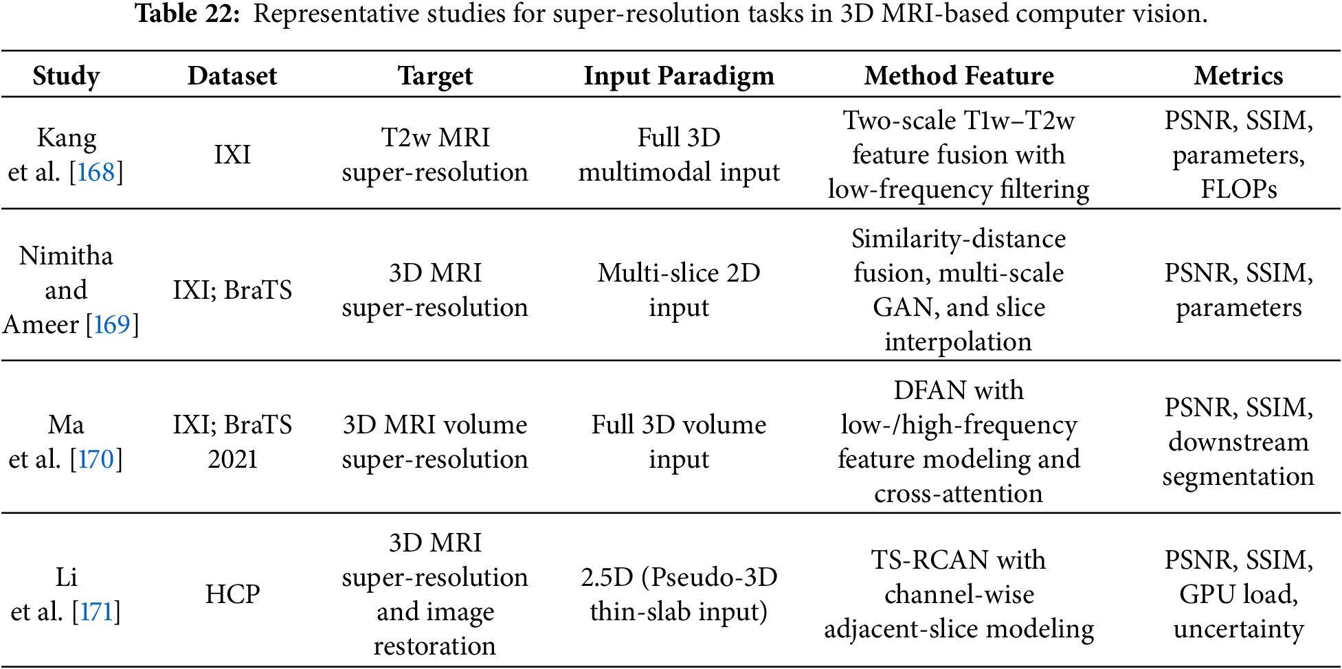
Overall, recent MRI super-resolution methods are moving toward stronger anatomical detail preservation, better inter-slice consistency, and more clinically feasible computation. GAN-based methods can improve perceptual sharpness but require careful validation to avoid hallucinated structures. Transformer- and frequency-aware methods can enhance global context and high-frequency recovery, but may increase computational cost. 2.5D methods provide a practical compromise between 2D efficiency and 3D spatial awareness.

5.5 Summary of Downstream Computer Vision Tasks

Section 5 reviewed four major downstream tasks in 3D MRI-based computer vision: detection/diagnosis, segmentation, reconstruction/restoration, and super-resolution. These tasks differ in their prediction targets, output structures, and evaluation criteria. Detection and diagnosis generally produce subject-, lesion-, or region-level predictions and are commonly evaluated using accuracy, sensitivity, specificity, AUC, precision, recall, and F1-score. Segmentation is usually assessed using overlap-based metrics, such as the Dice score and IoU/Jaccard index, together with boundary-based metrics, such as the Hausdorff distance or HD95 and Average Surface Distance. Reconstruction, restoration, and super-resolution focus on recovering or enhancing image and volume data, with performance often reported using error-based metrics such as MSE, NMSE, MAE, and RMSE, together with image-quality metrics such as PSNR and SSIM and, where appropriate, visual assessment.

Across these tasks, the choice of input paradigm remains closely tied to the expected output. Full 3D models are advantageous when volumetric continuity is central to the task, particularly in segmentation, reconstruction, and super-resolution. In contrast, 2D, 2.5D, and multi-view strategies remain useful when computation, model reuse, training data, or annotation availability constrain the use of fully volumetric processing.

Taken together, 3D MRI analysis is better understood as a family of task-specific pipelines than as a single unified problem. Detection and diagnosis emphasize discriminative representation, segmentation depends on spatial delineation, reconstruction and restoration prioritize image fidelity, and super-resolution aims to recover resolution and anatomical detail. This task-level distinction is important because the same MRI volume may require different input representations, model designs, and evaluation criteria depending on the intended application.

6  Current Status and Future Directions

6.1 Current Status of 3D MRI-Based Computer Vision

The studies reviewed in the previous sections show that 3D MRI-based computer vision has developed into a multi-task research field covering detection/diagnosis, segmentation, reconstruction/restoration, and super-resolution. These tasks have benefited from the rapid progress of CNNs, U-Net variants, transformers, generative models, diffusion models, self-supervised learning, and multimodal fusion. Publicly available datasets such as BraTS, ADNI, OASIS, IXI, HCP, OAI, and fastMRI have also provided important empirical foundations for benchmarking and method development.

However, a central observation emerging from this review is that the use of 3D MRI data remains only partially aligned with the intrinsic structure of MRI volumes. In many studies, MRI is technically available as a volumetric image, but the model input is still organized as 2D slices, selected views, cropped patches, or global volumes without explicit structural reasoning. This is understandable because 3D MRI volumes are computationally expensive, heterogeneous across scanners and protocols, and often difficult to annotate. Nevertheless, it also means that the full potential of 3D MRI as a spatial, volumetric, and anatomically continuous data source has not yet been fully exploited.

This limitation is especially evident when comparing the nature of MRI data with the way downstream tasks are formulated. A 3D MRI volume is not only a collection of image intensities. It contains spatial continuity, anatomical orientation, tissue boundaries, lesion morphology, volumetric extent, and inter-organ or intra-organ relationships. Yet many existing pipelines reduce this rich structure to task-specific labels, masks, or image-quality scores. Therefore, future research should pay more attention not only to network architecture, but also to how MRI data are represented, sampled, viewed, localized, interacted with, and connected to clinical information.

6.2 From Global Image-Level Prediction to Lesion-Centered Representation

An important future direction is to move from global image-level prediction toward lesion-centered and structure-aware representation. In many detection or diagnosis studies, 3D MRI is treated as a whole-volume input for binary or multi-class classification, such as disease diagnosis, tumor grading, or disease-stage prediction. This formulation is easy to implement and fits standard classification networks, but it differs from object detection in natural images, where the target object is usually localized through bounding boxes, region proposals, or instance-level annotations.

This issue is especially relevant to brain tumor MRI. BraTS provides multimodal 3D MRI volumes with voxel-level tumor annotations, and tumor lesions have clear spatial properties such as boundary, shape, volume, and distribution. These annotations can support three-dimensional contour, surface, or region-based analysis. However, many diagnosis-oriented studies still use the whole image or large patches as input and optimize a global classification objective. Such models may capture disease-related signals, but they often provide limited lesion-level localization, explanation, or explicit modeling of tumor morphology.

Segmentation partly addresses this problem by separating lesion from background tissue. However, a voxel-wise mask does not automatically provide a structured lesion representation. It identifies where the lesion is, but does not necessarily describe its geometry, boundary pattern, multi-view appearance, growth tendency, or spatial relationship with surrounding anatomy. Future studies may therefore explore intermediate representations between segmentation and diagnosis, such as lesion-centered graphs, tumor-surface features, boundary-aware descriptors, volumetric shape embeddings, and region-specific diagnostic models.

For tumor-related detection and diagnosis, this shift may improve both interpretability and clinical relevance. Instead of relying only on global MRI volumes, models could first identify lesion regions and then extract features related to tumor margin, necrotic core, edema distribution, enhancing rim, mass effect, and adjacency to critical structures. This design is closer to clinical reasoning, where radiologists assess not only whether a lesion exists, but also its location, margin, enhancement pattern, internal heterogeneity, and relationship with nearby anatomy.

Data scarcity, annotation cost, and class imbalance also influence the transition from global image-level analysis to lesion-centered representation. Processing a volume as 2D slices can increase the apparent number of training samples and reduce the cost of model optimization, but slices from the same subject are highly correlated and do not provide independent subject-level evidence. Full 3D approaches preserve volumetric context but generally require more memory and, for segmentation tasks, costly voxel-level annotations. They may also be strongly affected by class imbalance because lesions often occupy only a small proportion of the complete MRI volume. In such settings, 2.5D inputs or lesion-centered 3D patches can provide a practical compromise by incorporating local spatial context while reducing the amount of background processed by the model. However, overly localized sampling may remove clinically relevant global anatomy or introduce sampling bias. Future studies should therefore select the input paradigm together with the annotation level, lesion prevalence, and sampling strategy.

6.3 Beyond Orthogonal Slices: Arbitrary-Plane and Lesion-Oriented Views

Another promising direction is to move beyond fixed orthogonal views. Most slice-based and multi-view MRI methods rely on axial, coronal, and sagittal planes because these planes are standardized, easy to extract, and naturally aligned with the image grid. They also correspond to the routine viewing coordinates used in clinical interpretation. In contrast, oblique multiplanar reconstruction is generally used for targeted assessment along specific anatomical, pathological, or surgical orientations.

Nevertheless, the three orthogonal planes are not the only meaningful representations of a 3D MRI volume. After reconstruction and spatial normalization, MRI data can be resliced into arbitrary planes and visualized through oblique views, volume rendering, or surface rendering based on segmentation masks. This opens a less explored direction for computer vision: models may learn or generate task-adaptive views rather than relying only on predefined anatomical planes.

Such representations may be especially useful for lesion analysis. Tumors and other lesions often do not follow axial, coronal, or sagittal orientations. Their longest axis, invasive margin, edema spread, and spatial relationship with the ventricles, cortex, or neighboring structures may be more clearly represented from oblique or lesion-centered planes. Future methods could therefore define views according to lesion centroid, principal axes, boundary curvature, or surrounding anatomical landmarks, allowing the model to examine pathological structures from more informative directions.

This perspective also connects 2D, 2.5D, multi-view, and full 3D paradigms. Instead of treating these input types as fixed categories, MRI representation could be formulated as a view-selection problem. A model might dynamically sample informative planes from a 3D volume, including orthogonal planes, oblique planes, lesion-centered planes, and surface-oriented projections. Such a strategy could reduce computation compared with dense full 3D processing while preserving more lesion-specific geometry than conventional slice-wise input.

Arbitrary-plane reslicing, however, requires careful interpretation. Although technically feasible, different planes may not contain the same amount of acquired information, especially when thick-slice 2D acquisitions are resampled into a 3D volume. Future studies should distinguish clearly among acquired planes, reconstructed planes, orthogonal multiplanar reconstruction, oblique multiplanar reconstruction, and truly isotropic 3D acquisition. This distinction is important for model design, performance interpretation, and clinical validity.

Explainability should also be considered in relation to the underlying MRI input representation. For 2D models, Grad-CAM and saliency maps can identify influential regions within individual slices, but slice-wise explanations may not preserve volumetric continuity. In 2.5D and multi-view models, attribution results may further depend on how information is fused across adjacent slices or anatomical planes. Full 3D models can provide volumetric saliency or attention maps that are more directly aligned with three-dimensional anatomy, although their interpretation and visualization are more complex. A recent study using 3D structural MRI showed that models with similar classification performance could nevertheless rely on markedly different and not always anatomically plausible regions [172]. Future studies should therefore evaluate the spatial consistency, anatomical plausibility, and stability of explanations rather than presenting qualitative heatmaps alone.

6.4 Emerging Extensions of 3D MRI Representation

Beyond the established 2D, 2.5D, full 3D, and multi-view paradigms, the reviewed corpus also revealed several early-stage extensions of 3D MRI representation. Among the 178 included studies, one study explored interactive AR/VR (augmented reality/virtual reality)-based visualization and one investigated vision–language integration.

Khedir et al. [173] combined 3D tumor segmentation with interactive augmented-reality visualization, extending MRI analysis from voxel-level prediction to spatial presentation and user interaction. Such systems may support the inspection of lesion geometry and anatomical relationships, but their practical use depends on reliable segmentation, registration, surface reconstruction, real-time rendering, and clinically appropriate visualization.

Yoon et al. [174] integrated whole-volume 3D MRI with language-form clinical information from OASIS-3 and OASIS-4 through contrastive vision–language learning. This approach extends the representation problem from image-only modeling to the alignment of volumetric MRI with clinical text and metadata. Future multimodal systems may further combine MRI with radiology reports, demographic variables, cognitive assessments, electronic health records, radiomic features, genomic information, and pathology data. Such integration may support more comprehensive disease characterization, but it also introduces challenges related to missing modalities, heterogeneous data scales, cross-modal inconsistency, temporal mismatch, and interpretability.

Foundation models [175] and self-supervised learning [176] represent related model- and training-level developments that may further influence how 3D MRI representations are learned and transferred. Large-scale or self-supervised pretraining may reduce dependence on dense annotations and improve transfer across datasets and downstream tasks. However, such transfer should not be assumed from internal validation alone, because differences in scanner hardware, acquisition protocols, preprocessing pipelines, disease distribution, and patient demographics may still produce substantial domain shifts at independent institutions. These approaches also do not replace the input paradigms examined in this review. Whether a model is pretrained, multimodal, or language-aligned, volumetric MRI must still be organized as 2D slices, limited inter-slice representations, full 3D volumes or patches, or multiple anatomical views. Future research should therefore examine how these emerging learning strategies interact with spatial representation, computational cost, volumetric-context preservation, and cross-dataset or multi-center generalization.

Overall, the small number of AR/VR and vision–language studies identified in the 178-study corpus suggests that interactive visualization and multimodal language integration remain exploratory directions. Foundation-model and self-supervised approaches may further broaden these emerging extensions, but their value for 3D MRI will still depend on an appropriate representation of the underlying volumetric data.

7  Conclusion and Limitations

This review examined recent 3D MRI-based computer vision studies from the perspectives of dataset families, input paradigms, downstream tasks, and evaluation practices. The reviewed literature was organized around four major input paradigms—2D, 2.5D, full 3D, and multi-view representations—and four broad task categories: detection/diagnosis, segmentation, reconstruction/restoration, and super-resolution.

The findings show that input representation is a central methodological choice in 3D MRI analysis. Full 3D modeling was the most frequently used paradigm, particularly for segmentation and reconstruction-related tasks. However, this pattern reflects its prevalence in the reviewed literature rather than evidence of universal superiority. Two-dimensional, 2.5D, and multi-view approaches remain valuable when computational resources, annotation availability, sample size, or deployment conditions are limited. The choice of input paradigm should therefore be made jointly with consideration of dataset characteristics, task requirements, and practical constraints.

Several limitations should be acknowledged. First, the review focused on peer-reviewed journal articles indexed in the Web of Science Core Collection between 2021 and 2026. Relevant conference papers, preprints, studies indexed only in other databases, and articles with insufficiently reported input strategies may therefore have been excluded. Second, the requirement for publicly available datasets may have underrepresented studies based on proprietary clinical data, and the resulting corpus was dominated by neuroimaging applications.

Third, no quantitative meta-analysis was performed because the included studies differed substantially in datasets, cohort composition, data splits, preprocessing procedures, outcome definitions, and evaluation metrics. Reported performance values were therefore not pooled or used to establish the comparative effectiveness of different models or input paradigms.

Fourth, a formal study-level risk-of-bias assessment was not conducted. The purpose of this review was to map methodological patterns rather than to estimate a common clinical or predictive effect, and the included studies covered heterogeneous tasks for which no single conventional risk-of-bias tool was applicable. Accordingly, the findings should be interpreted as descriptive patterns in the literature rather than as evidence that one model or representation strategy is superior. Potential concerns, including data leakage, limited external validation, incomplete reporting of preprocessing, and selective metric reporting, were considered narratively.

Finally, the use of dominant dataset, input, and task categories simplified studies involving multiple datasets, hybrid representations, or auxiliary objectives. Although this approach improved interpretability, it may have obscured some within-study complexity.

Overall, this review highlights that progress in 3D MRI-based computer vision depends not only on model architecture but also on task-appropriate data representation. Future research should emphasize transparent preprocessing, independent and external validation, consistent reporting of uncertainty and computational cost, and clinically interpretable evaluation.

Acknowledgement: Not applicable.

Funding Statement: This work was supported by the Institute of Information & communications Technology Planning & Evaluation (IITP) under the Leading Generative AI Human Resources Development (IITP-2026-RS-2026-25544527) grant funded by the Korea government (MSIT). This work was supported by the research fund of Hanyang University (HY-2025-1110).

Author Contributions: The authors confirm contribution to the paper as follows: conceptualization, Jiawei Tian and Kyungtae Kang; methodology, Jiawei Tian and Kyungtae Kang; validation, Jiawei Tian and Kyungtae Kang; formal analysis, Jiawei Tian; investigation, Jiawei Tian; resources, Kyungtae Kang; data curation, Jiawei Tian; writing—original draft preparation, Jiawei Tian; writing—review and editing, Jiawei Tian and Kyungtae Kang; visualization, Jiawei Tian; supervision, Kyungtae Kang; project administration, Kyungtae Kang; funding acquisition, Kyungtae Kang. All authors reviewed and approved the final version of the manuscript.

Availability of Data and Materials: Not applicable.

Ethics Approval: Not applicable.

Conflicts of Interest: The authors declare no conflicts of interest.

Supplementary Materials: The supplementary material is available online at https://www.techscience.com/doi/10.32604/cmes.2026.087740/s1. PRISMA checklists are available in the supplementary material.

References

1. Rajiah PS, François CJ, Leiner T. Cardiac MRI: State of the art. Radiology. 2023;307(3):e223008. doi:10.1148/radiol.223008. [Google Scholar] [CrossRef]

2. Fernandes MC, Yildirim O, Woo S, Vargas HA, Hricak H. The role of MRI in prostate cancer: Current and future directions. Magn Reson Mater Phys Biol Med. 2022;35(4):503–21. doi:10.1007/s10334-022-01006-6. [Google Scholar] [CrossRef]

3. Fernandes MC, Gollub MJ, Brown G. The importance of MRI for rectal cancer evaluation. Surg Oncol. 2022;43(3):101739. doi:10.1016/j.suronc.2022.101739. [Google Scholar] [CrossRef]

4. Dorfner FJ, Patel JB, Kalpathy-Cramer J, Gerstner ER, Bridge CP. A review of deep learning for brain tumor analysis in MRI. npj Precis Oncol. 2025;9(1):2. doi:10.1038/s41698-024-00789-2. [Google Scholar] [CrossRef]

5. Lonchakov A, Sinitca A, Kaplun D. Computer vision-based medical imaging techniques: Past, present, and future. IEEE Access. 2026;14(2):14193–212. doi:10.1109/access.2026.3654393. [Google Scholar] [CrossRef]

6. Lundervold AS, Lundervold A. An overview of deep learning in medical imaging focusing on MRI. Z Für Med Phys. 2019;29(2):102–27. doi:10.1016/j.zemedi.2018.11.002. [Google Scholar] [CrossRef]

7. Jabbar M, Jamil U, Younas M, Zafar B. An explainability-aware transformer framework for brain tumor segmentation and classification using MRI. Comput Model Eng Sci. 2026;147(1):40. doi:10.32604/cmes.2026.080241. [Google Scholar] [CrossRef]

8. Wang H, Huang H, Wu J, Li N, Gu K, Wu X. Semi-supervised segmentation of cardiac chambers from LGE-CMR using feature consistency awareness. BMC Cardiovasc Disord. 2024;24(1):571. doi:10.1186/s12872-024-04250-x. [Google Scholar] [CrossRef]

9. Pang Y, Li Y, Liang J, Chen H, Hu Y, Wang Q. SegTom: A 3D volumetric medical image segmentation framework for thoracoabdominal multi-organ anatomical structures. IEEE J Biomed Health Inform. 2026;30(1):551–63. doi:10.1109/jbhi.2025.3606266. [Google Scholar] [CrossRef]

10. Zhao Z, Yeoh PSQ, Zuo X, Chuah JH, Chow CO, Wu X, et al. Vision transformer-equipped convolutional neural networks for automated Alzheimer’s disease diagnosis using 3D MRI scans. Front Neurol. 2024;15:1490829. doi:10.3389/fneur.2024.1490829. [Google Scholar] [CrossRef]

11. Demir F, Akbulut Y, Taşcı B, Demir K. Improving brain tumor classification performance with an effective approach based on new deep learning model named 3ACL from 3D MRI data. Biomed Signal Process Control. 2023;81(1):104424. doi:10.1016/j.bspc.2022.104424. [Google Scholar] [CrossRef]

12. Salam A, Abrar M, Anwer RW, Amin F, Ullah F, de la Torre I, et al. Channel-attention DenseNet with dilated convolutions for MRI brain tumor classification. Comput Model Eng Sci. 2025;145(2):2457–79. doi:10.32604/cmes.2025.072765. [Google Scholar] [CrossRef]

13. Wei R, Chen J, Liang B, Chen X, Men K, Dai J. Real-time 3D MRI reconstruction from cine-MRI using unsupervised network in MRI-guided radiotherapy for liver cancer. Med Phys. 2023;50(6):3584–96. doi:10.1002/mp.16141. [Google Scholar] [CrossRef]

14. Lin J, Miao QI, Surawech C, Raman SS, Zhao K, Wu HH, et al. High-resolution 3D MRI with deep generative networks via novel slice-profile transformation super-resolution. IEEE Access. 2023;11:95022–36. doi:10.1109/access.2023.3307577. [Google Scholar] [CrossRef]

15. Li H, Jia Y, Zhu H, Han B, Du J, Liu Y. Multi-level feature extraction and reconstruction for 3D MRI image super-resolution. Comput Biol Med. 2024;171(6):108151. doi:10.1016/j.compbiomed.2024.108151. [Google Scholar] [CrossRef]

16. Zhu F, Wang S, Li D, Li Q. Similarity attention-based CNN for robust 3D medical image registration. Biomed Signal Process Control. 2023;81(8):104403. doi:10.1016/j.bspc.2022.104403. [Google Scholar] [CrossRef]

17. Balluff B, Heeren RMA, Race AM. An overview of image registration for aligning mass spectrometry imaging with clinically relevant imaging modalities. J Mass Spectrom Adv Clin Lab. 2022;23(2):26–38. doi:10.1016/j.jmsacl.2021.12.006. [Google Scholar] [CrossRef]

18. Litjens G, Kooi T, Bejnordi BE, Setio AAA, Ciompi F, Ghafoorian M, et al. A survey on deep learning in medical image analysis. Med Image Anal. 2017;42(13):60–88. doi:10.1016/j.media.2017.07.005. [Google Scholar] [CrossRef]

19. Li M, Zhou C, Cao S. 2D, 2.5D, or 3D? Comparing dimensional approaches in deep neural networks for 3D medical image analysis. J Imaging Inform Med. 2026. doi:10.1007/s10278-025-01827-6. [Google Scholar] [CrossRef]

20. Sabanci K, Aslan B, Aslan MF. Medical image segmentation methods: A decision-guided survey covering 2D/3D CNNs, transformers, VLMs, SAM-based models and diffusion approaches. Bioengineering. 2026;13(5):555. doi:10.3390/bioengineering13050555. [Google Scholar] [CrossRef]

21. de Oliveira JVS, Vieira DF, da Silva MP, Fernandes DL, Ribeiro MHF, Oliveira HN. Strategies for deep learning in volumetric medical imaging: a survey. In: Proceedings of the 2025 38th SIBGRAPI Conference on Graphics, Patterns and Images (SIBGRAPI); 2025 Sep 30–Oct 3; Salvador, Brazil. doi:10.1109/sibgrapi67909.2025.11223395. [Google Scholar] [CrossRef]

22. Almansour AGM, Alshomrani F, Almutairi ATM, Alalwany E, Alshuhri MS, Alshaari H, et al. DA-ViT: Deformable attention vision transformer for Alzheimer’s disease classification from MRI scans. Comput Model Eng Sci. 2025;144(2):2395–418. doi:10.32604/cmes.2025.069661. [Google Scholar] [CrossRef]

23. Rani S, Singh BK, Koundal D, Athavale VA. Localization of stroke lesion in MRI images using object detection techniques: A comprehensive review. Neurosci Inform. 2022;2(3):100070. doi:10.1016/j.neuri.2022.100070. [Google Scholar] [CrossRef]

24. Shirly S, Ramesh K. Review on 2D and 3D MRI image segmentation techniques. Curr Med Imaging Rev. 2019;15(2):150–60. doi:10.2174/1573405613666171123160609. [Google Scholar] [CrossRef]

25. Kim S, Park H, Park SH. A review of deep learning-based reconstruction methods for accelerated MRI using spatiotemporal and multi-contrast redundancies. Biomed Eng Lett. 2024;14(6):1221–42. doi:10.1007/s13534-024-00425-9. [Google Scholar] [CrossRef]

26. Zhou H, Huang Y, Li Y, Zhou Y, Zheng Y. Blind super-resolution of 3D MRI via unsupervised domain transformation. IEEE J Biomed Health Inform. 2023;27(3):1409–18. doi:10.1109/JBHI.2022.3232511. [Google Scholar] [CrossRef]

27. Zhou SK, Greenspan H, Davatzikos C, Duncan JS, van Ginneken B, Madabhushi A, et al. A review of deep learning in medical imaging: Imaging traits, technology trends, case studies with progress highlights, and future promises. Proc IEEE Inst Electr Electron Eng. 2021;109(5):820–38. doi:10.1109/JPROC.2021.3054390. [Google Scholar] [CrossRef]

28. Singh SP, Wang L, Gupta S, Goli H, Padmanabhan P, Gulyás B. 3D deep learning on medical images: A review. Sensors. 2020;20(18):5097. doi:10.3390/s20185097. [Google Scholar] [CrossRef]

29. Wang T, Lei Y, Fu Y, Wynne JF, Curran WJ, Liu T, et al. A review on medical imaging synthesis using deep learning and its clinical applications. J Appl Clin Med Phys. 2021;22(1):11–36. doi:10.1002/acm2.13121. [Google Scholar] [CrossRef]

30. Gan HS, Ramlee MH, Wang Z, Shimizu A. A review on medical image segmentation: Datasets, technical models, challenges and solutions. WIREs Data Min Knowl. 2025;15(1):e1574. doi:10.1002/widm.1574. [Google Scholar] [CrossRef]

31. Sarkis-Onofre R, Catalá-López F, Aromataris E, Lockwood C. How to properly use the PRISMA statement. Syst Rev. 2021;10(1):117. doi:10.1186/s13643-021-01671-z. [Google Scholar] [CrossRef]

32. Guan X, Yang G, Ye J, Yang W, Xu X, Jiang W, et al. 3D AGSE-VNet: An automatic brain tumor MRI data segmentation framework. BMC Med Imaging. 2022;22(1):6. doi:10.1186/s12880-021-00728-8. [Google Scholar] [CrossRef]

33. Wu S, Chen Z, Sun P. 3D U-TFA: a deep convolutional neural network for automatic segmentation of glioblastoma. Biomed Signal Process Control. 2025;99(4):106829. doi:10.1016/j.bspc.2024.106829. [Google Scholar] [CrossRef]

34. Fan Y, Wang C, Zhang X, Yue Z, Chen J, Zhou Q. A causality-guided lightweight model for 3D multi-modal brain tumor segmentation. Biomed Signal Process Control. 2026;122(2):110392. doi:10.1016/j.bspc.2026.110392. [Google Scholar] [CrossRef]

35. Alnaggar OAMF, Jagadale BN, Narayan SH, Saif MAN. Brain tumor detection from 3D MRI using hyper-layer convolutional neural networks and hyper-heuristic extreme learning machine. Concurrency Computat Pract Exper. 2022;34(24):e7215. doi:10.1002/cpe.7215. [Google Scholar] [CrossRef]

36. Aminian M, Khotanlou H. CapsNet-based brain tumor segmentation in multimodal MRI images using inhomogeneous voxels in Del vector domain. Multimed Tools Appl. 2022;81(13):17793–815. doi:10.1007/s11042-022-12403-3. [Google Scholar] [CrossRef]

37. Alsubaie MG, Luo S, Shaukat K, Zhang W, Li J. A novel deep learning approach for Alzheimer’s disease detection: Attention-driven convolutional neural networks with multi-activation fusion. AI. 2025;6(12):324. doi:10.3390/ai6120324. [Google Scholar] [CrossRef]

38. Chang TA, Yu CC, Wang YH, Lei ZP, Chang CH. A hierarchical multi-modal fusion framework for Alzheimer’s disease classification using 3D MRI and clinical biomarkers. Electronics. 2026;15(2):367. doi:10.3390/electronics15020367. [Google Scholar] [CrossRef]

39. Turrisi R, Pati S, Pioggia G, Tartarisco G. Adapting to evolving MRI data: A transfer learning approach for Alzheimer’s disease prediction. NeuroImage. 2025;307(2):121016. doi:10.1016/j.neuroimage.2025.121016. [Google Scholar] [CrossRef]

40. Nagarjuna Reddy G, Nagi Reddy K. Alz-SAENet: A deep sparse autoencoder based model for Alzheimer’s classification. Int J Adv Comput Sci Appl. 2022;13(10):340–8. doi:10.14569/ijacsa.2022.0131041. [Google Scholar] [CrossRef]

41. Lim BY, Lai KW, Haiskin K, Kulathilake KASH, Ong ZC, Hum YC, et al. Deep learning model for prediction of progressive mild cognitive impairment to Alzheimer’s disease using structural MRI. Front Aging Neurosci. 2022;14:876202. doi:10.3389/fnagi.2022.876202. [Google Scholar] [CrossRef]

42. Almajalid R, Zhang M, Shan J. Fully automatic knee bone detection and segmentation on three-dimensional MRI. Diagnostics. 2022;12(1):123. doi:10.3390/diagnostics12010123. [Google Scholar] [CrossRef]

43. Berrimi M, Jennane R. MVMI: Multi-view multi-instance network for the detection of knee osteoarthritis. Biomed Signal Process Control. 2026;113(1):108794. doi:10.1016/j.bspc.2025.108794. [Google Scholar] [CrossRef]

44. Zhang H, Wang P, Xie Y, Yin H. Joint segmentation and diagnosis of knee osteoarthritis from 3d MRI using a transformer-based hybrid network. J Mech Med Biol. 2025;25(10):2540110. doi:10.1142/s0219519425401104. [Google Scholar] [CrossRef]

45. Hewlett M, Petrov I, Johnson PM, Drangova M. Deep-learning-based motion correction using multichannel MRI data: A study using simulated artifacts in the fastMRI dataset. NMR Biomed. 2024;37(10):e5179. doi:10.1002/nbm.5179. [Google Scholar] [CrossRef]

46. Zhao R, Yaman B, Zhang Y, Stewart R, Dixon A, Knoll F, et al. fastMRI+, clinical pathology annotations for knee and brain fully sampled magnetic resonance imaging data. Sci Data. 2022;9(1):152. doi:10.1038/s41597-022-01255-z. [Google Scholar] [CrossRef]

47. Bakas S, Akbari H, Sotiras A, Bilello M, Rozycki M, Kirby JS, et al. Advancing the cancer genome atlas glioma MRI collections with expert segmentation labels and radiomic features. Sci Data. 2017;4(1):170117. doi:10.1038/sdata.2017.117. [Google Scholar] [CrossRef]

48. Menze BH, Jakab A, Bauer S, Kalpathy-Cramer J, Farahani K, Kirby J, et al. The multimodal brain tumor image segmentation benchmark (BRATS). IEEE Trans Med Imaging. 2015;34(10):1993–2024. doi:10.1109/tmi.2014.2377694. [Google Scholar] [CrossRef]

49. Bakas S, Reyes M, Jakab A, Bauer S, Rempfler M, Crimi A, et al. Identifying the best machine learning algorithms for brain tumor segmentation, progression assessment, and overall survival prediction in the BRATS challenge. arXiv:1811.02629. 2018. [Google Scholar]

50. Antonelli M, Reinke A, Bakas S, Farahani K, Kopp-Schneider A, Landman BA, et al. The medical segmentation decathlon. Nat Commun. 2022;13(1):4128. doi:10.1038/s41467-022-30695-9. [Google Scholar] [CrossRef]

51. Isensee F, Jaeger PF, Kohl SAA, Petersen J, Maier-Hein KH. nnU-Net: a self-configuring method for deep learning-based biomedical image segmentation. Nat Methods. 2021;18(2):203–11. doi:10.1038/s41592-020-01008-z. [Google Scholar] [CrossRef]

52. Liew SL, Anglin JM, Banks NW, Sondag M, Ito KL, Kim H, et al. A large, open source dataset of stroke anatomical brain images and manual lesion segmentations. Sci Data. 2018;5(1):180011. doi:10.1038/sdata.2018.11. [Google Scholar] [CrossRef]

53. Liew SL, Tavenner BP, Donnelly MR, Zavaliangos-Petropulu A, Jeong JN, Barisano G, et al. A large, curated, open-source stroke neuroimaging dataset to improve lesion segmentation algorithms. Sci Data. 2022;9(1):320. doi:10.1038/s41597-022-01401-7. [Google Scholar] [CrossRef]

54. Mueller SG, Weiner MW, Thal LJ, Petersen RC, Jack C, Jagust W, et al. The Alzheimer’s disease neuroimaging initiative. Neuroimaging Clin N Am. 2005;15(4):869–77. doi:10.1016/j.nic.2005.09.008. [Google Scholar] [CrossRef]

55. Jack CR Jr, Bernstein MA, Fox NC, Thompson P, Alexander G, Harvey D, et al. The Alzheimer’s disease neuroimaging initiative (ADNIMRI methods. J Magn Reson Imaging. 2008;27(4):685–91. doi:10.1002/jmri.21049. [Google Scholar] [CrossRef]

56. Weiner MW, Veitch DP, Aisen PS, Beckett LA, Cairns NJ, Green RC, et al. The Alzheimer’s disease neuroimaging initiative 3: continued innovation for clinical trial improvement. Alzheimers Dement. 2017;13(5):561–71. doi:10.1016/j.jalz.2016.10.006. [Google Scholar] [CrossRef]

57. Zhou J, Wei Y, Li X, Zhou W, Tao R, Hua Y, et al. A deep learning model for early diagnosis of Alzheimer’s disease combined with 3D CNN and video swin transformer. Sci Rep. 2025;15(1):23311. doi:10.1038/s41598-025-05568-y. [Google Scholar] [CrossRef]

58. Marcus DS, Wang TH, Parker J, Csernansky JG, Morris JC, Buckner RL. Open access series of imaging studies (OASIScross-sectional MRI data in young, middle aged, nondemented, and demented older adults. J Cogn Neurosci. 2007;19(9):1498–507. doi:10.1162/jocn.2007.19.9.1498. [Google Scholar] [CrossRef]

59. Marcus DS, Fotenos AF, Csernansky JG, Morris JC, Buckner RL. Open access series of imaging studies: longitudinal MRI data in nondemented and demented older adults. J Cogn Neurosci. 2010;22(12):2677–84. doi:10.1162/jocn.2009.21407. [Google Scholar] [CrossRef]

60. LaMontagne PJ, Benzinger TL, Morris JC, Keefe S, Hornbeck R, Xiong C, et al. OASIS-3: longitudinal neuroimaging, clinical, and cognitive dataset for normal aging and Alzheimer disease. medRxiv. 2019. doi:10.1101/2019.12.13.19014902. [Google Scholar] [CrossRef]

61. Malone IB, Cash D, Ridgway GR, MacManus DG, Ourselin S, Fox NC, et al. MIRIAD—public release of a multiple time point Alzheimer’s MR imaging dataset. Neuroimage. 2013;70:33–6. doi:10.1016/j.neuroimage.2012.12.044. [Google Scholar] [CrossRef]

62. IXI Dataset: Information eXtraction from Images [Internet]. London, UK: Brain Development; 2002 [cited 2026 Jul 1]. Available from: https://brain-development.org/ixi-dataset/. [Google Scholar]

63. Glasser MF, Sotiropoulos SN, Wilson JA, Coalson TS, Fischl B, Andersson JL, et al. The minimal preprocessing pipelines for the human connectome project. NeuroImage. 2013;80(6):105–24. doi:10.1016/j.neuroimage.2013.04.127. [Google Scholar] [PubMed] [CrossRef]

64. Marcus DS, Harwell J, Olsen T, Hodge M, Glasser MF, Prior F, et al. Informatics and data mining tools and strategies for the human connectome project. Front Neuroinform. 2011;5:4. doi:10.3389/fninf.2011.00004. [Google Scholar] [CrossRef]

65. Peterfy CG, Schneider E, Nevitt M. The osteoarthritis initiative: Report on the design rationale for the magnetic resonance imaging protocol for the knee. Osteoarthr Cartil. 2008;16(12):1433–41. doi:10.1016/j.joca.2008.06.016. [Google Scholar] [CrossRef]

66. Eckstein F, Wirth W, Nevitt MC. Recent advances in osteoarthritis imaging—The osteoarthritis initiative. Nat Rev Rheumatol. 2012;8(10):622–30. doi:10.1038/nrrheum.2012.113. [Google Scholar] [CrossRef]

67. Solomon E, Johnson PM, Tan Z, Tibrewala R, Lui YW, Knoll F, et al. FastMRI breast: A publicly available radial k-space dataset of breast dynamic contrast-enhanced MRI. Radiol Artif Intell. 2025;7(1):e240345. doi:10.1148/ryai.240345. [Google Scholar] [CrossRef]

68. Tibrewala R, Dutt T, Tong A, Ginocchio L, Lattanzi R, Keerthivasan MB, et al. FastMRI Prostate: A public, biparametric MRI dataset to advance machine learning for prostate cancer imaging. Sci Data. 2024;11(1):404. doi:10.1038/s41597-024-03252-w. [Google Scholar] [CrossRef]

69. Zbontar J, Knoll F, Sriram A, Murrell T, Huang Z, Muckley MJ, et al. fastMRI: An open dataset and benchmarks for accelerated MRI. arXiv:1811.08839. 2018. [Google Scholar]

70. Knoll F, Zbontar J, Sriram A, Muckley MJ, Bruno M, Defazio A, et al. fastMRI: A publicly available raw k-space and DICOM dataset of knee images for accelerated MR image reconstruction using machine learning. Radiol Artif Intell. 2020;2(1):e190007. doi:10.1148/ryai.2020190007. [Google Scholar] [CrossRef]

71. Zhang Y, Liao Q, Ding L, Zhang J. Bridging 2D and 3D segmentation networks for computation-efficient volumetric medical image segmentation: an empirical study of 2.5D solutions. Comput Med Imaging Graph. 2022;99(11):102088. doi:10.1016/j.compmedimag.2022.102088. [Google Scholar] [CrossRef]

72. Yang J, Huang X, He Y, Xu J, Yang C, Xu G, et al. Reinventing 2D convolutions for 3D images. IEEE J Biomed Health Inform. 2021;25(8):3009–18. doi:10.1109/jbhi.2021.3049452. [Google Scholar] [CrossRef]

73. Ronneberger O, Fischer P, Brox T. U-Net: convolutional networks for biomedical image segmentation. In: Medical Image Computing and Computer-Assisted Intervention–MICCAI 2015. Berlin/Heidelberg, Germany: Springer; 2015. p. 234–41. doi:10.1007/978-3-319-24574-4_28. [Google Scholar] [CrossRef]

74. Çiçek Ö., Abdulkadir A, Lienkamp SS, Brox T, Ronneberger O. 3D U-Net: learning dense volumetric segmentation from sparse annotation. In: Medical Image Computing and Computer-Assisted Intervention–MICCAI 2016. Berlin/Heidelberg, Germany: Springer; 2016. p. 424–32. doi:10.1007/978-3-319-46723-8_49. [Google Scholar] [CrossRef]

75. Milletari F, Navab N, Ahmadi SA. V-net: fully convolutional neural networks for volumetric medical image segmentation. In: Proceedings of the 2016 Fourth International Conference on 3D Vision (3DV); 2016 Oct 25–28; Stanford, CA, USA. doi:10.1109/3dv.2016.79. [Google Scholar] [CrossRef]

76. Vu MH, Grimbergen G, Nyholm T, Löfstedt T. Evaluation of multislice inputs to convolutional neural networks for medical image segmentation. Med Phys. 2020;47(12):6216–31. doi:10.1002/mp.14391. [Google Scholar] [CrossRef]

77. Shams S, Platania R, Zhang J, Kim J, Lee K, Park SJ. Deep generative breast cancer screening and diagnosis. In: Medical Image Computing and Computer Assisted Intervention–MICCAI 2018. Berlin/Heidelberg, Germany: Springer; 2018. p. 859–67. doi:10.1007/978-3-030-00934-2_95. [Google Scholar] [CrossRef]

78. Wachinger C, Reuter M, Klein T. DeepNAT: deep convolutional neural network for segmenting neuroanatomy. Neuroimage. 2018;170(3):434–45. doi:10.1016/j.neuroimage.2017.02.035. [Google Scholar] [CrossRef]

79. Henschel L, Conjeti S, Estrada S, Diers K, Fischl B, Reuter M. FastSurfer—A fast and accurate deep learning based neuroimaging pipeline. NeuroImage. 2020;219(7):117012. doi:10.1016/j.neuroimage.2020.117012. [Google Scholar] [CrossRef]

80. Guha Roy A, Conjeti S, Navab N, Wachinger C. QuickNAT: a fully convolutional network for quick and accurate segmentation of neuroanatomy. NeuroImage. 2019;186(5):713–27. doi:10.1016/j.neuroimage.2018.11.042. [Google Scholar] [CrossRef]

81. Ali Hassen O, Omar Abter S, Abdulhussein AA, Darwish SM, Ibrahim YM, Sheta W. Nature-inspired level set segmentation model for 3D-MRI brain tumor detection. Comput Mater Contin. 2021;68(1):961–81. doi:10.32604/cmc.2021.014404. [Google Scholar] [CrossRef]

82. Sharma R, Goel T, Tanveer M, Murugan R. FDN-ADNet: fuzzy LS-TWSVM based deep learning network for prognosis of the Alzheimer’s disease using the sagittal plane of MRI scans. Appl Soft Comput. 2022;115(3):108099. doi:10.1016/j.asoc.2021.108099. [Google Scholar] [CrossRef]

83. Mamikov S, Yakhiya Z, Omarov B, Mamashov Y, Aliyeva A, Tursynbek B. Feature pyramid network with dual-decoder supervision for accurate stroke lesion localization in multi-modal brain MRI. Int J Adv Comput Sci Appl. 2025;16(10):499–509. doi:10.14569/ijacsa.2025.0161052. [Google Scholar] [CrossRef]

84. Srilakshmi V, Devarasetty P, Chetana VL, Vinta S, Kowtharapu R. Alzheimer’s disease staging using enhanced inception-ResNet-V2 and improved XceptionNet models for 3D MRI classification and segmentation. J Neurosci Methods. 2026;432(8):110767. doi:10.1016/j.jneumeth.2026.110767. [Google Scholar] [CrossRef]

85. Gautam P, Singh M. 3-1-3 Weight averaging technique-based performance evaluation of deep neural networks for Alzheimer’s disease detection using structural MRI. Biomed Phys Eng Express. 2024;10(6):5027. doi:10.1088/2057-1976/ad72f7. [Google Scholar] [CrossRef]

86. Alirr OI. A large-kernel and scale-aware 2D CNN with boundary refinement for multimodal ischemic stroke lesion segmentation. Eng. 2026;7(2):59. doi:10.3390/eng7020059. [Google Scholar] [CrossRef]

87. Ahanger AB, Aalam SW, Assad A, Ahmad Macha M, Bhat MR. Alzhinet: an explainable self-attention based classification model to detect Alzheimer from 3D volumetric MRI data. Int J Syst Assur Eng Manag. 2024. doi:10.1007/s13198-024-02377-w. [Google Scholar] [CrossRef]

88. Li Y, Zhu H, Hou T, Chen N, Huang B, Lu W, et al. A parallel dual-domain crossing network combining attention enhancement and multimodal fusion for MRI reconstruction. Biomed Signal Process Control. 2025;110(4):108326. doi:10.1016/j.bspc.2025.108326. [Google Scholar] [CrossRef]

89. Zhu J, Zou L, Xie X, Xu R, Tian Y, Zhang B. 2.5D deep learning based on multi-parameter MRI to differentiate primary lung cancer pathological subtypes in patients with brain metastases. Eur J Radiol. 2024;180(12):111712. doi:10.1016/j.ejrad.2024.111712. [Google Scholar] [CrossRef]

90. Pang S, Chen Y, Shi X, Wang R, Dai M, Zhu X, et al. Interpretable 2.5D network by hierarchical attention and consistency learning for 3D MRI classification. Pattern Recognit. 2025;164(5):111539. doi:10.1016/j.patcog.2025.111539. [Google Scholar] [CrossRef]

91. Ottesen JA, Yi D, Tong E, Iv M, Latysheva A, Saxhaug C, et al. 2.5D and 3D segmentation of brain metastases with deep learning on multinational MRI data. Front Neuroinform. 2022;16:1056068. doi:10.3389/fninf.2022.1056068. [Google Scholar] [CrossRef]

92. Karimzadeh M, Seyedarabi H, Jodeiri A, Afrouzian R. Enhanced brain stroke lesion segmentation in MRI using a 2.5D transformer backbone U-Net model. Brain Sci. 2025;15(8):778. doi:10.3390/brainsci15080778. [Google Scholar] [CrossRef]

93. Soelistiono S. A longitudinal and explainable 2.5D deep learning framework for Alzheimer’s disease progression using ADNI MRI. NeuroImage Rep. 2026;6(2):100342. doi:10.1016/j.ynirp.2026.100342. [Google Scholar] [CrossRef]

94. Hu Z, Li Y, Wang Z, Zhang S, Hou W. Conv-Swinformer: integration of CNN and shift window attention for Alzheimer’s disease classification. Comput Biol Med. 2023;164(2022):107304. doi:10.1016/j.compbiomed.2023.107304. [Google Scholar] [CrossRef]

95. Mohan D, Venugopal U, Joseph N, Govindarajan K. Inter and intra slice reduction in brain tumor segmentation. Trait Du Signal. 2023;40(1):395–400. doi:10.18280/ts.400141. [Google Scholar] [CrossRef]

96. Rashid AH, Gupta A, Gupta J, Tanveer M. Biceph-net: A robust and lightweight framework for the diagnosis of Alzheimer’s disease using 2D-MRI scans and deep similarity learning. IEEE J Biomed Health Inform. 2023;27(3):1205–13. doi:10.1109/JBHI.2022.3174033. [Google Scholar] [CrossRef]

97. Rahim N, Abuhmed T, Mirjalili S, El-Sappagh S, Muhammad K. Time-series visual explainability for Alzheimer’s disease progression detection for smart healthcare. Alex Eng J. 2023;82(5):484–502. doi:10.1016/j.aej.2023.09.050. [Google Scholar] [CrossRef]

98. Karthik R, Menaka R, Hariharan M, Won D. Ischemic lesion segmentation using ensemble of multi-scale region aligned CNN. Comput Methods Programs Biomed. 2021;200(suppl 1):105831. doi:10.1016/j.cmpb.2020.105831. [Google Scholar] [CrossRef]

99. Ma B, Sun Q, Ma Z, Li B, Cao Q, Wang Y, et al. DTASUnet: a local and global dual transformer with the attention supervision U-network for brain tumor segmentation. Sci Rep. 2024;14(1):28379. doi:10.1038/s41598-024-78067-1. [Google Scholar] [CrossRef]

100. Sohail N, Anwar SM. A modified U-Net based framework for automated segmentation of hippocampus region in brain MRI. IEEE Access. 2022;10:31201–9. doi:10.1109/access.2022.3159618. [Google Scholar] [CrossRef]

101. Ghaffari M, Samarasinghe G, Jameson M, Aly F, Holloway L, Chlap P, et al. Automated post-operative brain tumour segmentation: A deep learning model based on transfer learning from pre-operative images. Magn Reson Imaging. 2022;86:28–36. doi:10.1016/j.mri.2021.10.012. [Google Scholar] [CrossRef]

102. Liang J, Yang C, Zeng L. 3D PSwinBTS: an efficient transformer-based Unet using 3D parallel shifted windows for brain tumor segmentation. Digit Signal Process. 2022;131(5):103784. doi:10.1016/j.dsp.2022.103784. [Google Scholar] [CrossRef]

103. Akbar AS, Fatichah C, Suciati N, Za’in C. Yaru3DFPN: A lightweight modified 3D UNet with feature pyramid network and combine thresholding for brain tumor segmentation. Neural Comput Appl. 2024;36(13):7529–44. doi:10.1007/s00521-024-09475-7. [Google Scholar] [CrossRef]

104. Ghribi F, Hamdaoui F. A novel 3D U-net-vision transformer hybrid with multi-scale fusion for precision multimodal brain tumor segmentation in 3D MRI. Electronics. 2025;14(18):3604. doi:10.3390/electronics14183604. [Google Scholar] [CrossRef]

105. Li H, Qi X, Hu Y, Zhang J. Arouse-net: enhancing glioblastoma segmentation in multi-parametric MRI with a custom 3D convolutional neural network and attention mechanism. Mathematics. 2025;13(1):160. doi:10.3390/math13010160. [Google Scholar] [CrossRef]

106. Chen YT, Ahmad N, Aurangzeb K. Enhancing 3D U-Net with residual and squeeze-and-excitation attention mechanisms for improved brain tumor segmentation in multimodal MRI. Comput Model Eng Sci. 2025;144(1):1197–224. doi:10.32604/cmes.2025.066580. [Google Scholar] [CrossRef]

107. Alarjani M, Almuaibed A. Optimizing a 3D convolutional neural network to detect Alzheimer’s disease based on MRI. PeerJ Comput Sci. 2025;11(3):e3129. doi:10.7717/peerj-cs.3129. [Google Scholar] [CrossRef]

108. Chen W, Cai C, Tan X, Lv R, Zhang J, Du G. MAUNet: A mixed attention U-Net with spatial multi-dimensional convolution and contextual feature calibration for 3D brain tumor segmentation in multimodal MRI. Front Neurosci. 2025;19:1682603. doi:10.3389/fnins.2025.1682603. [Google Scholar] [CrossRef]

109. Zhou Z, Yu X, Huang W, Qiu S, Humayoo M, Li H, et al. Comprehensive exploiting local and global features for brain tumor segmentation: a gated dual-branch hybrid attention mechanism. Biomed Signal Process Control. 2025;110(9):108285. doi:10.1016/j.bspc.2025.108285. [Google Scholar] [CrossRef]

110. Cui H, Ruan Z, Xu Z, Luo X, Dai J, Geng D. ResMT: a hybrid CNN-transformer framework for glioma grading with 3D MRI. Comput Electr Eng. 2024;120(8):109745. doi:10.1016/j.compeleceng.2024.109745. [Google Scholar] [CrossRef]

111. Karimi H, Hamghalam M. Segmentation of 3D MRI using 2D convolutional neural networks in infants’ brain. Multimed Tools Appl. 2024;83(11):33511–26. doi:10.1007/s11042-023-16790-z. [Google Scholar] [CrossRef]

112. Chen X, Jiang S, Guo L, Chen Z, Zhang C. Whole brain segmentation method from 2.5D brain MRI slice image based on Triple U-Net. Visual Comput. 2023;39(1):255–66. doi:10.1007/s00371-021-02326-9. [Google Scholar] [CrossRef]

113. Li C, Gao Z, Chen X, Zheng X, Zhang X, Lin CY. Ensemble network using oblique coronal MRI for Alzheimer’s disease diagnosis. NeuroImage. 2025;310(1):121151. doi:10.1016/j.neuroimage.2025.121151. [Google Scholar] [CrossRef]

114. Mossa AA, Çevİk U. Ensemble learning of multiview CNN models for survival time prediction of brain tumor patients using multimodal MRI scans. Turk J Elec Eng & Comp Sci. 2021;29(2):616–31. doi:10.3906/elk-2002-175. [Google Scholar] [CrossRef]

115. Alp S, Akan T, Bhuiyan MS, Disbrow EA, Conrad SA, Vanchiere JA, et al. Joint transformer architecture in brain 3D MRI classification: its application in Alzheimer’s disease classification. Sci Rep. 2024;14(1):8996. doi:10.1038/s41598-024-59578-3. [Google Scholar] [CrossRef]

116. Rahim N, Ahmad N, Ullah W, Bedi J, Jung Y. Early progression detection from MCI to AD using multi-view MRI for enhanced assisted living. Image Vis Comput. 2025;157(10):105491. doi:10.1016/j.imavis.2025.105491. [Google Scholar] [CrossRef]

117. Islam M, Hasan MJ, Mahdy MRC. CQ-CNN: a lightweight hybrid classical-quantum convolutional neural network for Alzheimer’s disease detection using 3D structural brain MRI. PLoS One. 2025;20(9):e0331870. doi:10.1371/journal.pone.0331870. [Google Scholar] [CrossRef]

118. Ben Ahmed K, Hall LO, Goldgof DB, Gatenby R. Ensembles of convolutional neural networks for survival time estimation of high-grade glioma patients from multimodal MRI. Diagnostics. 2022;12(2):345. doi:10.3390/diagnostics12020345. [Google Scholar] [CrossRef]

119. Hamoud M, Chekima NEI, Hima A, Kholladi NH. An automated cascade framework for glioma prognosis via segmentation, multi-feature fusion and classification techniques. Biomed Phys Eng Express. 2025;11(3):5027. doi:10.1088/2057-1976/add26c. [Google Scholar] [CrossRef]

120. Negied N, SeragEldin A. Automatic detection of Alzheimer disease from 3D MRI images using deep CNNs. Int J Adv Comput Sci Appl. 2022;13(12):477–82. doi:10.14569/ijacsa.2022.0131258. [Google Scholar] [CrossRef]

121. Biswas R, Gini JR. Multi-class classification of Alzheimer’s disease detection from 3D MRI image using ML techniques and its performance analysis. Multimed Tools Appl. 2024;83(11):33527–54. doi:10.1007/s11042-023-16519-y. [Google Scholar] [CrossRef]

122. Guida C, Zhang M, Shan J. Knee osteoarthritis classification using 3D CNN and MRI. Appl Sci. 2021;11(11):5196. doi:10.3390/app11115196. [Google Scholar] [CrossRef]

123. Ahanger AB, Aalam SW, Assad A, Ahmad Macha M, Bhat MR. Assessing glioma grading with self-attention: comparative analysis of the diagnostic potential of different MRI sequences. Int J Syst Assur Eng Manag. 2024. doi:10.1007/s13198-024-02401-z. [Google Scholar] [CrossRef]

124. Ashames MMA, Ergin S, Gerek ON, Yavuz HS. Attention-enhanced 3D residual networks for knee abnormality classification. Expert Syst Appl. 2026;298(3):129858. doi:10.1016/j.eswa.2025.129858. [Google Scholar] [CrossRef]

125. Bao S, Zheng F, Jiang L, Wang Q, Lyu Y. TA-SSM net: tri-directional attention and structured state-space model for enhanced MRI-Based diagnosis of Alzheimer’s disease and mild cognitive impairment. BMC Med Imaging. 2025;25(1):309. doi:10.1186/s12880-025-01836-5. [Google Scholar] [CrossRef]

126. Barstuğan M. An effective flowchart for multimodal brain tumor binary classification with ranked 3D texture features. Sci Rep. 2025;15(1):30531. doi:10.1038/s41598-025-11240-2. [Google Scholar] [PubMed] [CrossRef]

127. Castellano G, Esposito A, Lella E, Montanaro G, Vessio G. Automated detection of Alzheimer’s disease: a multi-modal approach with 3D MRI and amyloid PET. Sci Rep. 2024;14(1):5210. doi:10.1038/s41598-024-56001-9. [Google Scholar] [CrossRef]

128. Aggarwal R, Sounderajah V, Martin G, Ting DSW, Karthikesalingam A, King D, et al. Diagnostic accuracy of deep learning in medical imaging: a systematic review and meta-analysis. npj Digit Med. 2021;4(1):65. doi:10.1038/s41746-021-00438-z. [Google Scholar] [CrossRef]

129. Mosquera C, Ferrer L, Milone DH, Luna D, Ferrante E. Class imbalance on medical image classification: towards better evaluation practices for discrimination and calibration performance. Eur Radiol. 2024;34(12):7895–903. doi:10.1007/s00330-024-10834-0. [Google Scholar] [CrossRef]

130. Rehman ZU, Awang MK, Ali G, Hamza M, Ali T, Ayaz M, et al. 3D-MobiBrainNet: multi-class Alzheimer’s disease classification using 3D brain magnetic resonance imaging. Ain Shams Eng J. 2025;16(11):103714. doi:10.1016/j.asej.2025.103714. [Google Scholar] [CrossRef]

131. Montaha S, Azam S, Rafid AKMRH, Hasan MZ, Karim A, Islam A. TimeDistributed-CNN-LSTM: A hybrid approach combining CNN and LSTM to classify brain tumor on 3D MRI scans performing ablation study. IEEE Access. 2022;10(4):60039–59. doi:10.1109/access.2022.3179577. [Google Scholar] [CrossRef]

132. Tack A, Shestakov A, Lüdke D, Zachow S. A multi-task deep learning method for detection of meniscal tears in MRI data from the osteoarthritis initiative database. Front Bioeng Biotechnol. 2021;9:747217. doi:10.3389/fbioe.2021.747217. [Google Scholar] [CrossRef]

133. Berrimi M, Hans D, Jennane R. A semi-supervised multiview-MRI network for the detection of knee osteoarthritis. Comput Med Imaging Graph. 2024;114(6):102371. doi:10.1016/j.compmedimag.2024.102371. [Google Scholar] [CrossRef]

134. Berrimi M, Anwar SM, Jennane R. A three dimensional joint multiview, multi-task, multimodal network for knee injuries classification. Eng Appl Artif Intell. 2026;167(4):113902. doi:10.1016/j.engappai.2026.113902. [Google Scholar] [CrossRef]

135. Abadian-Zadeh FS, Mohammadi MR, Soryani M. Weakly supervised brain tumour segmentation with label propagation and level set loss. IET Image Process. 2025;19(1):13289. doi:10.1049/ipr2.13289. [Google Scholar] [CrossRef]

136. Zhou M, Li J, Guo Y. Multi-level channel-spatial attention and light-weight scale-fusion network (MCSLF-Netmulti-level channel-spatial attention and light-weight scale-fusion transformer for 3D brain tumor segmentation. Quant Imaging Med Surg. 2025;15(7):6301–25. doi:10.21037/qims-2025-354. [Google Scholar] [CrossRef]

137. Lairedj KI, Chama Z, Bagdaoui A, Larguech S, Menni Y, Becheikh N, et al. Advanced brain tumor segmentation in magnetic resonance imaging via 3D U-Net and generalized Gaussian mixture model-based preprocessing. Comput Model Eng Sci. 2025;144(2):2419–43. doi:10.32604/cmes.2025.069396. [Google Scholar] [CrossRef]

138. Shan Qing Yeoh P, Bing L, Li Goh S, Hasikin K, Wu X, Chai Hum Y, et al. An efficient neural network for segmenting multiple joint tissues from knee MRI with hyperparameter optimization: data from the osteoarthritis initiative. IEEE Access. 2024;12:123757–70. doi:10.1109/access.2024.3454374. [Google Scholar] [CrossRef]

139. Soh WK, Yuen HY, Rajapakse JC. HUT: Hybrid UNet transformer for brain lesion and tumour segmentation. Heliyon. 2023;9(12):e22412. doi:10.1016/j.heliyon.2023.e22412. [Google Scholar] [CrossRef]

140. Kaur G, Rana PS, Arora V. Deep learning and machine learning-based early survival predictions of glioblastoma patients using pre-operative three-dimensional brain magnetic resonance imaging modalities. Int J Imaging Syst Tech. 2023;33(1):340–61. doi:10.1002/ima.22804. [Google Scholar] [CrossRef]

141. Berkcan B, Kayıkçıoğlu T. Enhanced 3D DenseNet with CDC for multimodal brain tumor segmentation. Appl Sci. 2026;16(3):1572. doi:10.3390/app16031572. [Google Scholar] [CrossRef]

142. El Badaoui R, Bonmati Coll E, Psarrou A, Asaturyan HA, Villarini B. Enhanced CATBraTS for brain tumour semantic segmentation. J Imaging. 2025;11(1):8. doi:10.3390/jimaging11010008. [Google Scholar] [CrossRef]

143. Muthusivarajan R, Celaya A, Yung JP, Long JP, Viswanath SE, Marcus DS, et al. Evaluating the relationship between magnetic resonance image quality metrics and deep learning-based segmentation accuracy of brain tumors. Med Phys. 2024;51(7):4898–906. doi:10.1002/mp.17059. [Google Scholar] [CrossRef]

144. Cao G, Yang Z, Liang W, Zhang S, Zhong T, Mao H, et al. LCMF-Net: a lightweight collaborative multimodal fusion network for brain tumor segmentation. Neural Netw. 2026;195:108257. doi:10.1016/j.neunet.2025.108257. [Google Scholar] [CrossRef]

145. Müller D, Soto-Rey I, Kramer F. Towards a guideline for evaluation metrics in medical image segmentation. BMC Res Notes. 2022;15(1):210. doi:10.1186/s13104-022-06096-y. [Google Scholar] [CrossRef]

146. Eelbode T, Bertels J, Berman M, Vandermeulen D, Maes F, Bisschops R, et al. Optimization for medical image segmentation: theory and practice when evaluating with dice score or jaccard index. IEEE Trans Med Imaging. 2020;39(11):3679–90. doi:10.1109/TMI.2020.3002417. [Google Scholar] [CrossRef]

147. Cox J, Liu P, Stolte SE, Yang Y, Liu K, See KB, et al. BrainSegFounder: towards 3D foundation models for neuroimage segmentation. Med Image Anal. 2024;97(1):103301. doi:10.1016/j.media.2024.103301. [Google Scholar] [CrossRef]

148. Cao J, Ren L, Deng A, Yu F, Liu L, Jiang M. MHC-Segnet: Mamba–Hadamard collaboration segmentation network for multimodal MRI brain tumor. Visual Comput. 2025;41(12):9459–70. doi:10.1007/s00371-025-03961-2. [Google Scholar] [CrossRef]

149. Deng J, Xie X. 3D interactive segmentation with semi-implicit representation and active learning. IEEE Trans Image Process. 2021;30:9402–17. doi:10.1109/tip.2021.3125491. [Google Scholar] [CrossRef]

150. Raza R, Ijaz Bajwa U, Mehmood Y, Waqas Anwar M, Jamal MH. dResU-Net: 3D deep residual U-Net based brain tumor segmentation from multimodal MRI. Biomed Signal Process Control. 2023;79(4):103861. doi:10.1016/j.bspc.2022.103861. [Google Scholar] [CrossRef]

151. Pedada KR, Bhujanga Rao A, Patro KK, Allam JP, Jamjoom MM, Abdel Samee N. A novel approach for brain tumour detection using deep learning based technique. Biomed Signal Process Control. 2023;82(2):104549. doi:10.1016/j.bspc.2022.104549. [Google Scholar] [CrossRef]

152. Xing Q, Li Z, Jing Y, Chen X. A 3D dual encoder mirror difference ResU-net for multimodal brain tumor segmentation. IEEE Access. 2025;13(3):1621–35. doi:10.1109/access.2024.3522682. [Google Scholar] [CrossRef]

153. Di Matteo A, Mahé Y, Leplaideur S, Bonan I, Bannier E, Galassi F. Deep learning and multi-modal MRI for the segmentation of sub-acute and chronic stroke lesions. Pattern Recognit Lett. 2026;199(2):225–31. doi:10.1016/j.patrec.2025.11.017. [Google Scholar] [CrossRef]

154. Yeoh PSQ, Goh SL, Hasikin K, Wu X, Lai KW. 3D efficient multi-task neural network for knee osteoarthritis diagnosis using MRI scans: data from the osteoarthritis initiative. IEEE Access. 2023;11:135323–33. doi:10.1109/access.2023.3338379. [Google Scholar] [CrossRef]

155. Muckley MJ, Riemenschneider B, Radmanesh A, Kim S, Jeong G, Ko J, et al. Results of the 2020 fastMRI challenge for machine learning MR image reconstruction. IEEE Trans Med Imaging. 2021;40(9):2306–17. doi:10.1109/tmi.2021.3075856. [Google Scholar] [CrossRef]

156. Chen Y, Schonlieb CB, Lio P, Leiner T, Dragotti PL, Wang G, et al. AI-based reconstruction for fast MRI—a systematic review and meta-analysis. Proc IEEE. 2022;110(2):224–45. doi:10.1109/jproc.2022.3141367. [Google Scholar] [CrossRef]

157. Ben Yedder H, Cardoen B, Hamarneh G. Deep learning for biomedical image reconstruction: a survey. Artif Intell Rev. 2021;54(1):215–51. doi:10.1007/s10462-020-09861-2. [Google Scholar] [CrossRef]

158. Singh D, Monga A, de Moura HL, Zhang X, Zibetti MVW, Regatte RR. Emerging trends in fast MRI using deep-learning reconstruction on undersampled k-space data: a systematic review. Bioengineering. 2023;10(9):1012. doi:10.3390/bioengineering10091012. [Google Scholar] [CrossRef]

159. Liu X, Pang Y, Sun X, Liu Y, Hou Y, Wang Z, et al. Image reconstruction for accelerated MR scan with faster Fourier convolutional neural networks. IEEE Trans Image Process. 2024;33(1):2966–78. doi:10.1109/TIP.2024.3388970. [Google Scholar] [CrossRef]

160. Wu JM, Yin SB, Jiang TX, Liu GS, Zhao XL. PALADIN: a novel plug-and-play 3D CS-MRI reconstruction method. Inverse Probl. 2025;41(3):035014. doi:10.1088/1361-6420/adb8c6. [Google Scholar] [CrossRef]

161. Safari M, Eidex Z, Pan S, Qiu RLJ, Yang X. Self-supervised adversarial diffusion models for fast MRI reconstruction. Med Phys. 2025;52(6):3888–99. doi:10.1002/mp.17675. [Google Scholar] [CrossRef]

162. Rudie JD, Gleason T, Barkovich MJ, Wilson DM, Shankaranarayanan A, Zhang T, et al. Clinical assessment of deep learning-based super-resolution for 3D volumetric brain MRI. Radiol Artif Intell. 2022;4(2):e210059. doi:10.1148/ryai.210059. [Google Scholar] [CrossRef]

163. Giraldo DL, Khan H, Pineda G, Liang Z, Lozano-Castillo A, Van Wijmeersch B, et al. Perceptual super-resolution in multiple sclerosis MRI. Front Neurosci. 2024;18:1473132. doi:10.3389/fnins.2024.1473132. [Google Scholar] [CrossRef]

164. de Farias EC, di Noia C, Han C, Sala E, Castelli M, Rundo L. Impact of GAN-based lesion-focused medical image super-resolution on the robustness of radiomic features. Sci Rep. 2021;11(1):21361. doi:10.1038/s41598-021-00898-z. [Google Scholar] [CrossRef]

165. Shen Q, Zhang X, Chen P, Zhong Z, Leung H, Wang S. Unfolding high-order correlations for interpretable multi-contrast MRI super-resolution. IEEE Trans Image Process. 2026;35:3466–78. doi:10.1109/TIP.2026.3673935. [Google Scholar] [CrossRef]

166. Amoros M, Curado M, Vicent JF. Evaluating super-resolution models in biomedical imaging: applications and performance in segmentation and classification. J Imaging. 2025;11(4):104. doi:10.3390/jimaging11040104. [Google Scholar] [CrossRef]

167. Zhao J, Hong T, Qi H, Zhou Z, Wang H. A lightweight 3D distillation volumetric transformer for 3D MRI super-resolution. IEEE J Biomed Health Inform. 2025;29(7):5083–94. doi:10.1109/jbhi.2025.3555603. [Google Scholar] [CrossRef]

168. Kang L, Tang B, Huang J, Li J. 3D-MRI super-resolution reconstruction using multi-modality based on multi-resolution CNN. Comput Meth Programs Biomed. 2024;248(28):108110. doi:10.1016/j.cmpb.2024.108110. [Google Scholar] [CrossRef]

169. Nimitha U, Ameer PM. MRI super-resolution using similarity distance and multi-scale receptive field based feature fusion GAN and pre-trained slice interpolation network. Magn Reson Imaging. 2024;110(5):195–209. doi:10.1016/j.mri.2024.04.021. [Google Scholar] [CrossRef]

170. Ma J, Yu H, Hua X, Du Z, Li Z, Lu Q, et al. DFAN: dual frequency-aware network for 3D MRI volume super-resolution. Biomed Signal Process Control. 2026;112(10):108499. doi:10.1016/j.bspc.2025.108499. [Google Scholar] [CrossRef]

171. Li H, Liu J, Schell M, Huang T, Lauer A, Schregel K, et al. Performance of a GPU- and time-efficient pseudo-3D network for magnetic resonance image super-resolution and motion artifact reduction. Sci Rep. 2026;16(1):9654. doi:10.1038/s41598-026-43804-1. [Google Scholar] [CrossRef]

172. Jelitzki J, Reichenbach A, Windberger A. Decision processes in 3D structural MRI schizophrenia classification evaluated with saliency maps. Sci Rep. 2026;16(1):18362. doi:10.1038/s41598-026-57667-z. [Google Scholar] [CrossRef]

173. Khedir M, Amara K, Dif N, Kerdjidj O, Atalla S, Ramzan N. BrainAR: automated brain tumor diagnosis with deep learning and 3D augmented reality visualization. IEEE Access. 2025;13(6):128639–53. doi:10.1109/access.2025.3590291. [Google Scholar] [CrossRef]

174. Yoon J, Park H, Kim M, Jeong H, Young Chun S, Ji S, et al. Clinical dementia rating classification using integrated vision and language information. IEEE Access. 2025;13:184602–17. doi:10.1109/access.2025.3624215. [Google Scholar] [CrossRef]

175. Zhang G, Gao Z, Duan C, Liu J, Lizhu Y, Liu Y, et al. A multi-modal foundation model for brain disease diagnosis and medical imaging. Patterns. 2026;7(6):101538. doi:10.1016/j.patter.2026.101538. [Google Scholar] [CrossRef]

176. Espis A, Marzi C, Diciotti S. NeuroBooster: A domain-informed self-supervised learning paradigm tailored for brain MRI analysis. IEEE J Biomed Health Inform. 2026. doi:10.1109/JBHI.2026.3708015. [Google Scholar] [CrossRef]