Multiple Sclerosis Predictions and Sensitivity Analysis Using Robust Models

1  Introduction

The exact causes of MS are still unknown in the medical community, and treatment methods are active research. As there is no known cure [1] and the disease affects patients differently, prescribing effective treatments is of paramount importance. The variation of symptoms and treatment response represents a strong motivation for a personalized treatment approach. Thus, it is important to identify the disease through risk modeling approaches the patient characteristics can influence treatment, enabling the choice given patient effects. Prediction models help in identifying and estimating the impact of patient, inspection, and setting characteristics on future health outcomes [2]. The main risk of patients is often the basis of heterogeneous treatment effects [3].

Multiple sclerosis (MS) is a disease of the central nervous system [4] with several subtypes. The most common subtype is relapsing-remitting Multiple Sclerosis (RRMS) [5]. Patients with RRMS present with intense symptoms (relapses) followed by periods without symptoms (remission) [6]. Several treatments are available [7] with direct patient responses, with each treatment having a very different safety profile.it is also important to monitor progression of the disease [8]. Patient and particular setting characteristics can be included in network meta-regression models [9,10] to make predictions for different treatments and subgroups of patients [2]. This approach presents computational and practical difficulties when many predictors are to be included in the model.

Studies such as [11] advocate a particular treatment based on the best results obtained by the treatment on average across a pool of patients. We use the dataset from this study to develop a robust machine-learning approach to treatment prescription.

While modern machine learning methods like random forests and SVMs are known for their high accuracy in healthcare predictions, K-means clustering remains a valuable and practical alternative. One of its biggest strengths is its ability to identify patient subgroups without needing labeled data, which is especially useful in real-world medical settings where labeled datasets can be limited. Unlike complex models, K-means produces clear and interpretable groupings that doctors can easily understand and apply in treatment decisions.

That said, newer AI models like GPT-4 and BioBERT have made impressive strides in healthcare analytics, particularly in processing large amounts of medical text and identifying intricate patterns. These models can uncover deep insights, but they often require massive labeled datasets and heavy computational resources, making them less accessible for some applications. A promising direction for future research would be to combine K-means clustering with deep learning techniques, aiming for a balance between accuracy and interpretability. This way, we can harness the strengths of both approaches to improve clinical decision-making while keeping the results transparent and actionable.

2  Motivation

MS treatments are used to manage disease progression often throughout the life of the patients. We believe machine learning approaches can provide accurate treatment choices based on individual patient characteristics, leading to higher chances of symptom remission. This paper focuses on building models and testing them against perturbation in the underlying data. Patient data is variable, challenging to measure, and prone to human input errors [12]. Moreover, incorrectly predicting MS treatment can cause serious side effects for the patient. For this reason, we believe robust models bring an essential benefit to treatment analysis.

3  Dataset

The dataset was obtained from the study [2], and it consists of 10,000 observations of patient utility data. The target variable is the best treatment, a categorical variable taking three possible values: (1) high-dose, (2) low-dose, or (3) no treatment. The predictors are the utilities (i.e., risks) of each side effect (e.g., 0.8 utility of cardio-pulmonary distress). They differ as patients are impacted differently by the same side effect (e.g., an older patient will have a higher negative impact from a cardiac arrest). A higher utility means a higher risk and worse impact of a particular side effect. These utilities are calculated in the study [11] with qualitative information and depend on relapse severity, the difference between lethal and non-lethal outcomes, and individual patient characteristics. We used stratified sampling to split the data into training (7000 observations) and testing (3000 observations) while preserving the proportions of the three values of the target variable (best treatment).

The treatment outcome is not directly observable in the data. It is not recorded how the patient reacted to the treatment, whether there were any side effects, and how the MS disease progressed. We can only observe the calculated utility that each of the three treatments has on each patient. For example, for patient I, the utility of high-dose treatment was 0.87, the utility of low-dose treatment was 0.65, and the utility of no treatment was 0.54. A higher utility of treatment means a greater benefit to the patient.

Moreover, the dataset itself has been obtained via simulations, and in reality, the patient utility data is difficult to calculate. Patient measurements could be imprecise (e.g., recorded incorrectly by the measurement device), or they could be inputted into the system incorrectly by nurses or physicians. Furthermore, they represent only a snapshot of a patient’s state obtained when we take measurements such as blood pressure. Finally, future patients may not present the same characteristics as past patients MS symptoms and treatment reactions vary widely across the patient population. In other words, we cannot fully assume that patient utilities in the train and test set are drawn from a common distribution. This represents a strong argument in favor of sensitivity analysis and robust models for treatment prescription.

4  Methodology

4.1 K-Means Predictive-Prescriptive Models

K-means clustering is the basic clustering to find groups of data or clusters in the dataset.

This dataset is unsuitable for an approach such as Optimal Prescriptive Trees due to the lack of treatment outcomes. We instead developed an unsupervised prescriptive-predictive method based on K-means clustering [13]. The process follows two steps:

Perform the K-means algorithm on the patients’ utilities

For each new patient, prescribe the most common treatment of the cluster he/she belongs to. This can be formulated via the following optimization problem:

We defined T as the number of new patients, here 3000 (patients in the test set), and n the number of previous patients here 7000 (patients in the train set), z_p the treatment to prescribe (1 for high-dose, 2 for low-dose, and 3 for no treatment) for new patient p, and y_i the best treatment evaluated for the previous patient i, hence we get the following formulation:

maxzp∈(1,2,3)∑P=1T∑i=1nwpi1zp=yi

This formulation can be linearized with the introduction of additional variables and a sufficiently large constant M to obtain the following mixed-integer optimization problem:

maxzp∈(1,2,3)∑P=1T∑i=1nwpi(1−qpi)

subject to wpi=1 if p and i are in the same cluster

Mqpi≥qpi1(zp−yi)+qpi2(yi−zp)≥0

qpi1+qpi2=1

qpi,qpi1,qpi2∈{0,1)

Results: We obtained a 0.64 out-of-sample accuracy with 20 clusters, which is equal to the baseline accuracy, as we explained in the results section. This value changes slightly with the number 1 of clusters but remains within 2% of 0.64 for 5 to 100 clusters. The challenge of the unbalanced dataset in terms of the target variable remains prevalent even when splitting the patients into numerous clusters; hence, a clustering approach did not bring significant value.

4.2 Predictive Models: CART, OCT, OCT-H

For a personalized treatment approach, we predict the best treatment based on adverse effects utilities. Study [2] simply proposes the most effective treatment on average (high-dose) to all patients and will represent a baseline for our predictions. The accuracy of the baseline is 0.64.

We focus solely on interpretable models: (classification and regression tree) CART [13], OCT [14], and OCT-H [15]. The initial challenge with all three models was that after cross-validation, they were never predicting class = 2 (low-dose treatment), as it is the lowest-occurring option in the dataset. This challenge, especially when dealing with diseases, is common as the major part of the target observation may not surely get you what you want [16]. This has been addressed by implementing penalty matrices or slightly compromising performance in favor of a model that predicts all three classes. We believe detecting low-dose cases is important, rather than defaulting to a high-dose, which can be potentially dangerous for the patient, or no treatment that does not address the symptoms.

4.2.1 Classification Trees

To develop an interpretable predictive model, we implemented a Classification and Regression Tree (CART) model as shown in Fig. 1. Through cross-validation, we selected min bucket = 35 and cp = 0.0025.

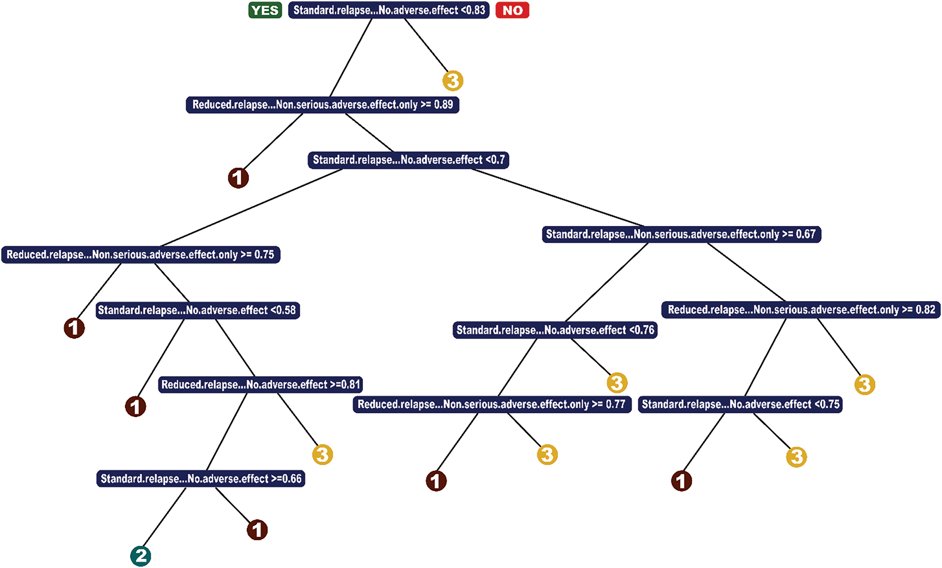
Figure 1: CART model

The minbucket parameter ensures that each terminal node contains at least 35 observations, preventing overfitting small variations in the data. A smaller value would create overly specific branches, reducing interpretability, while a larger value might oversimplify the model and obscure important distinctions. The chosen value strikes a balance between stability and capturing meaningful treatment patterns. The cp (complexity parameter) controls the pruning process by setting the minimum improvement in error required for a split. A smaller cp allows for deeper trees, capturing more nuanced patterns, while a larger cp aggressively prunes the tree, improving interpretability at the cost of potential underfitting. The selected cp = 0.0025 ensures a reasonable trade-off between complexity and interpretability.

The resulting model primarily splits on variables indicating the absence of serious adverse effects. Intuitively, this means the decision tree differentiates patients based on whether they are at risk for severe side effects (e.g., cardiac arrest, diabetes, cardio-pulmonary distress) rather than on specific types of side effects. From a treatment perspective, the model suggests that patients with a low risk of serious adverse effects should receive high-dose treatment (option 1), which aligns with medical intuition—these patients are least likely to experience complications from the strongest treatment.

To address the issue of underprediction for class = 2 (low-dose treatment)—a common problem in imbalanced datasets—we implemented a loss matrix. This over-penalized misclassification of low-dose cases ensured the model did not default to prescribing only high-dose or no treatment. This adjustment is crucial, as identifying cases where less aggressive treatment is sufficient can help minimize unnecessary risks for patients.

The final CART model achieved 70% accuracy, demonstrating a significant improvement over the baseline (64%). The key advantages of CART are its simplicity, computational efficiency, and interpretability, making it a practical choice for clinical decision-making. However, given its greedy nature in selecting splits, we further explored Optimal Classification Trees (OCT) to assess whether a more global optimization approach could yield additional benefits.

We implemented a loss matrix to ensure class = 2 (low-dose treatment) was being predicted by the model. As mentioned, this is because we believe less invasive treatment to be beneficial. We over-penalize misclassification of low-dose, and we also consider the trade-off between prescribing treatment when we should not go vs. under-prescribing. The best accuracy of a CART model was 70%. The advantage of CART is that it is a simple model, runs fast, and performs very similarly to OCT and OCT-H.

4.2.2 Optimal Classification Trees

We next attempted an OCT-model (Fig. 2), and ran cross-validation, obtaining the parameters minbucket = 35, cp = 0.003, and max depth = 4. Cross-validated accuracy was 0.71; however, we encountered the same issue of never predicting a low dose; therefore, we decided on a final model of depth 5 with an accuracy score of 0.70.

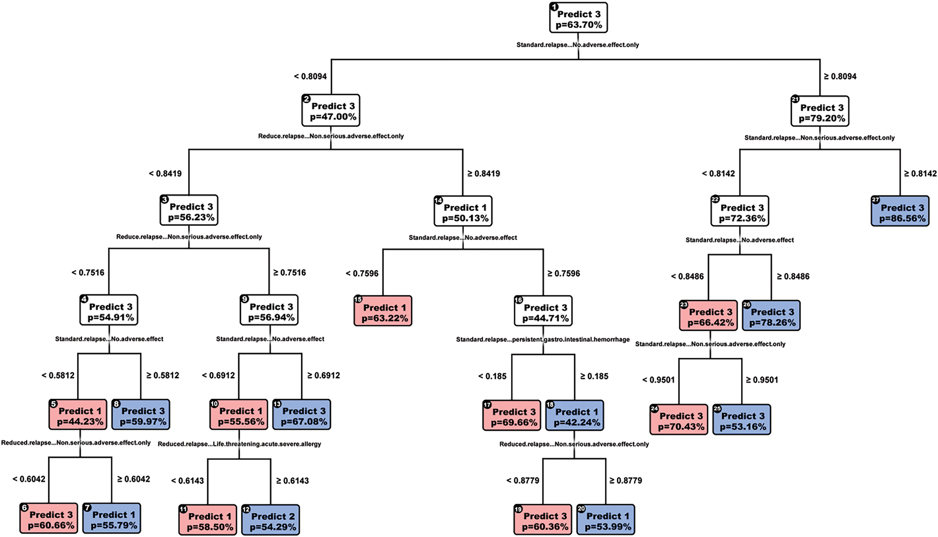
Figure 2: OCT-model

Like CART, the variables are split to detect the absence of serious adverse effects, yet we see new variables such as gastrointestinal hemorrhage, seizure, and cardio-pulmonary distress. OCT does not make greedy splits in the way CART does, enabling it to output splits across more features, providing us with richer information. OCT also is more interpretable than CART, having only five layers, as opposed to 7. Since the accuracy scores are the same, we favor OCT over CART.

4.2.3 Optimal Classification Trees with Hyperplanes

Finally, we looked at OCT-H as shown in Fig. 3, hoping to improve performance, yet the model performed very similarly to both CART and OCT, improving only to 0.71 accuracies. The chosen model also has depth = 5 instead of the cross-validated model with depth = 2. We chose this for the same reason that the cross-validated tree did not predict low-dose treatment.

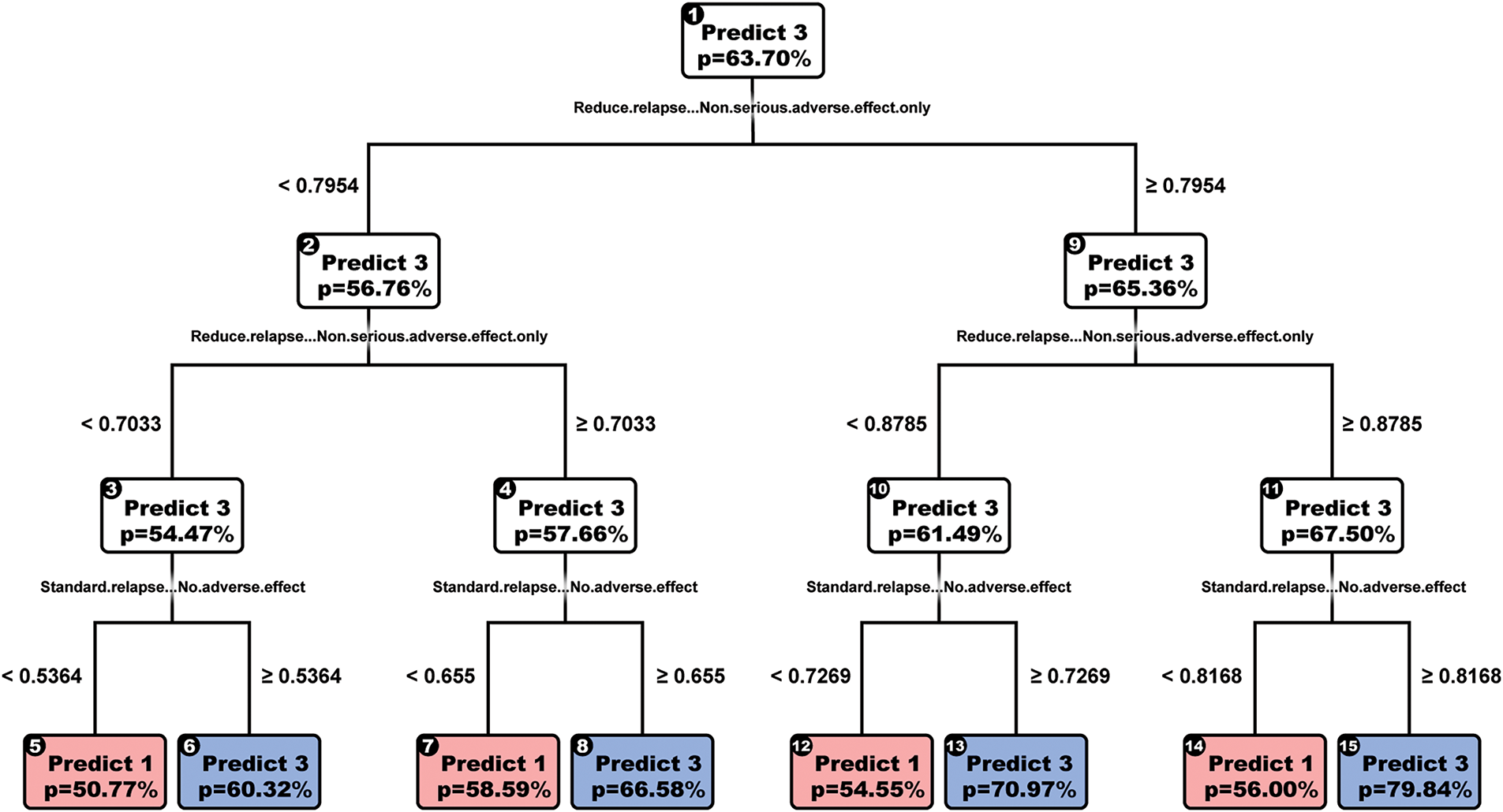
Figure 3: OCTH-model

The drawbacks of OCT-H are the reduced rate at which they can be interpreted (e.g., most splits have four variables) and the significant runtime for cross-validation (over 3 h).

4.2.4 Multinomial Logistic Regression

We also performed a multinomial logistic regression on this problem, giving an out-of-sample accuracy slightly lower, at 0.59. The main advantage of this method is that it can be robustified by adding a lasso regularized term. This model has a lower performance than the baseline (0.64); however, it has proven useful in the robustification process.

5  Sensitivity Analysis

The goal of sensitivity analysis was to test the models against changes in the underlying data and check the impact on accuracy as we increase the magnitude of changes. We first calculated the means mj and standard deviation σj of each predictor (patient utility) j. Then, we progressively perturbed the test dataset. For each feature column i, for each patient j, having the utility uij, we associate the perturbation pij. Hence, uij becomes u′ij = uij + pij where pij is generated randomly with the normal distribution of mean mj and standard deviation pσj where p is in the range of perturbation, up to 3 in our case. By progressively perturbing within 1σj, 2σj, and 3σj, we test how the accuracy changes at different stages.

5.1 K-Means Prescriptive-Predictive Model

The impact of the perturbation on the K-means predictive-prescriptive method gives us the following results as shown in Fig. 4:

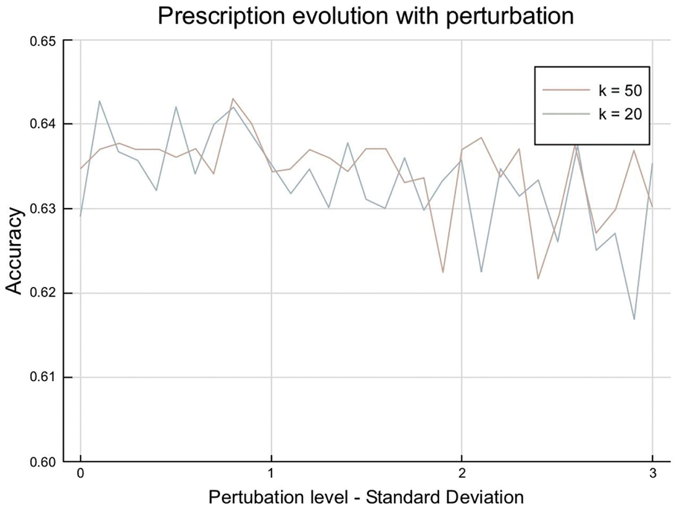
Figure 4: K-means perturbation impact

This shows an underlying characteristic of the problem: for low values of clusters, the most common treatment is the same for all clusters. These also correspond to this project’s reference study [1], where one treatment was given to all the patients. For a high number of clusters, the accuracy remains at levels of 0.62 and 0.64, which means we predict treatment 1 for most clusters but not all.

5.2 Sensitivity Analysis of the Tree Models

5.2.1 Sensitivity Evolution with the Tree Depth and Complexity

After building the initial models, we vary their tree depth in Fig. 5a and assess their sensitivity to out-of-sample perturbation.

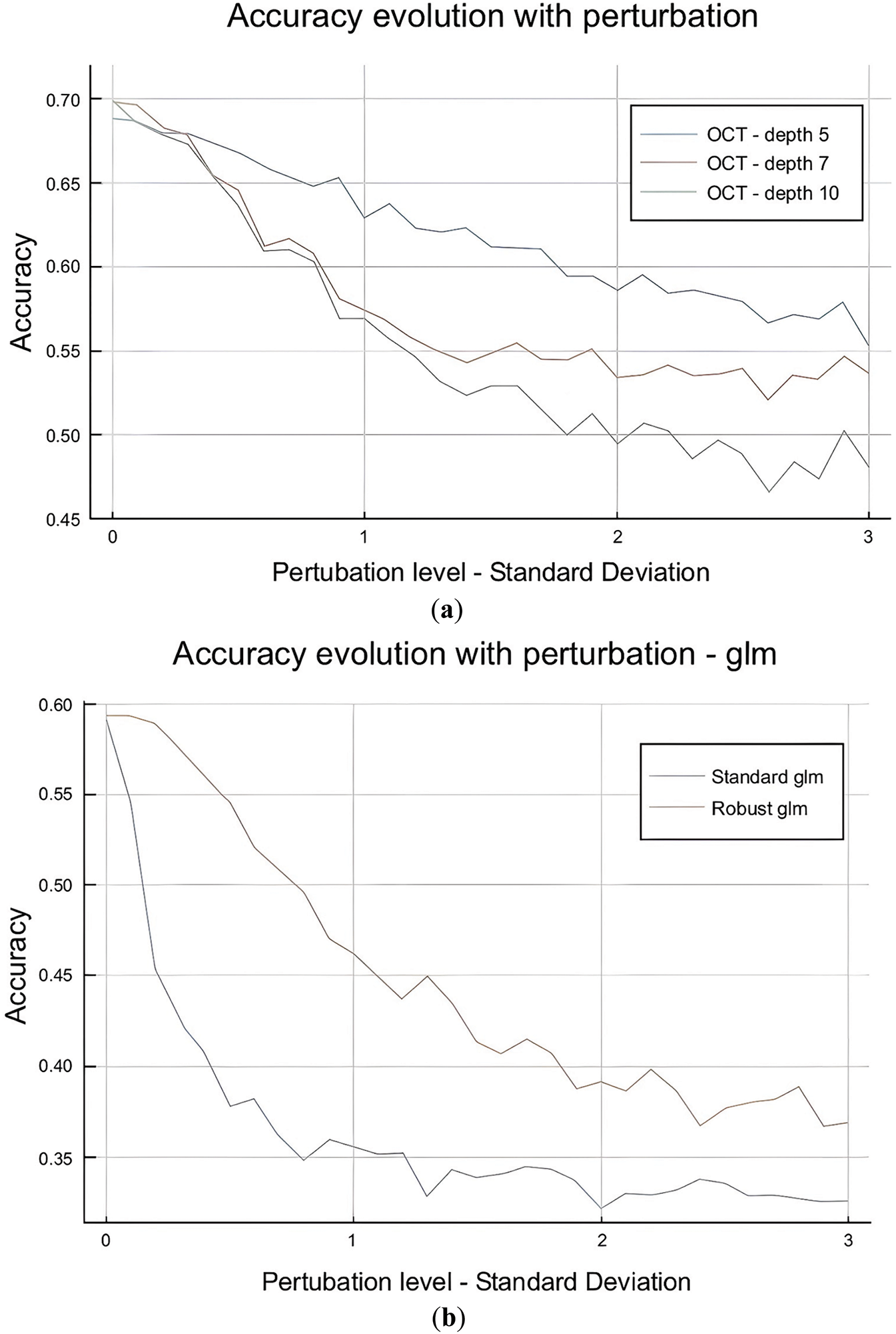
Figure 5: (a): OCT depth impact. (b): Perturbation impact: OCT vs. OCT-H performance

The OCT is highly sensitive to perturbation in the test set with the evolution of the perturbation range, with accuracy decreasing from 0.70 to 0.55 when the data is perturbed within a range of 3σ. The perturbation impact is higher for deeper trees, making sense as the deeper the tree is, the more complex it is and sensitive to external perturbations. Similarly, OCT-H is more sensitive to perturbations than OCT as show in Fig. 5b. This also matches our intuition as OCT-H is more complex and fits better the data in-sample but is sensitive to out-of-sample perturbations.

5.2.2 Sensitivity Evolution with the Number of Features Perturbed

Another approach is to assess the sensitivity evolution with the number of features perturbed. The first step was to identify which features to perturb. We already have the feature importance from CART and OCT as provided in Table 1 as well as a random forest model that we ran:

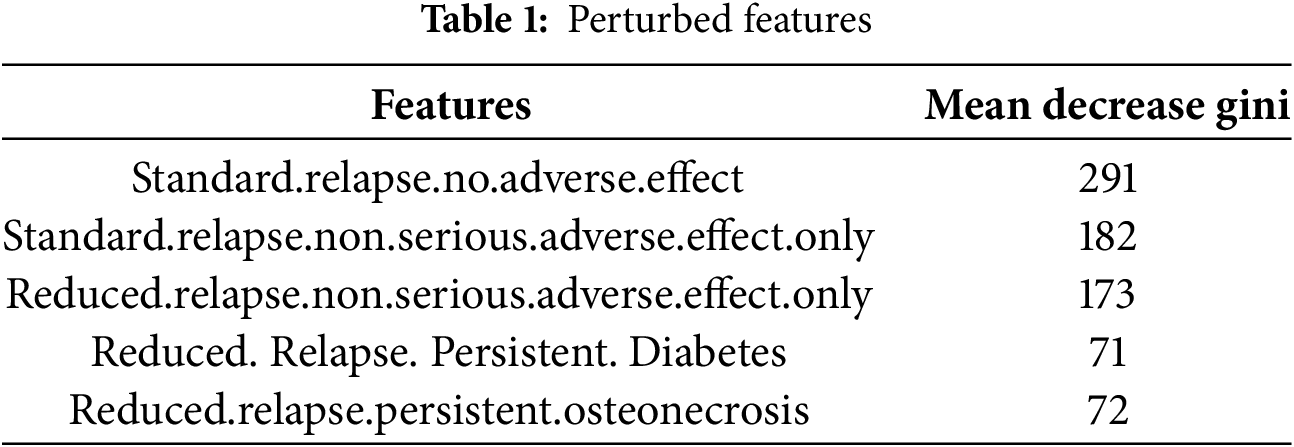
The top three features indicate no adverse effect or no serious adverse effect, conditioned by the progression of the MS disease (standard vs. reduced relapse). In essence, high values in these features signal a relatively healthy patient with a high chance of no adverse effect from the methylprednisolone treatment. This is different from the rest of the predictors, where high values indicate a high risk (e.g., diabetes). The aim is to verify if there is a correlation between the feature’s importance and the impact of its perturbation on the model’s performance.

In Fig. 6 below, the main three lines (blue, red, and green) correspond to perturbing the three features with the highest importance (as taken from the table above) at different perturbation levels. The other lines at the top of the chart highlight perturbation in the rest of the features, excluding the three most important ones. These give two very interesting insights. The first one is that only the three most important features influence the model’s performance, as there is almost no impact while perturbing a higher and higher number of features. These also could be seen in the perturbations, including all the features. This perturbation does not evolve a lot with the number of features, implying that the perturbation comes only from a sparse number of parameters. A second observation is that when the important features are excluded, whatever the perturbation intensity is in terms of the number of standard deviations, the impact remains the same. These observations enable us to conclude that our model will be very robust to out-of-sample perturbations if we precisely control the three most important features.

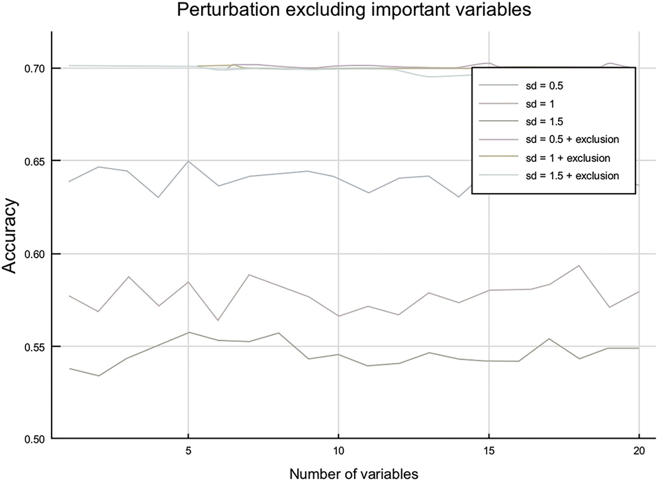
Figure 6: Perturbation by number of variables

We can also draw another interesting conclusion—the top three features are sufficient to predict the best treatment with high accuracy (e.g., CART split on these three features alone and achieved 0.70 accuracies). Currently, a high-dose treatment is prescribed to all patients, perhaps justified by the difficulty in measuring all 56 of the predictor variables. Since the top three features are sufficient, we could only measure those for each patient. In practice, this may prove challenging since the features are “no adverse effect”, which technically still implies we must look at all adverse effects. Yet, it is a valuable insight that if we find one single serious adverse effect, this is enough information to make a prediction.

6  Models Robustification and Results

6.1 Impact of Multinomial Logistic Regression

First, we assessed the performance of the multinomial logistic regression by introducing a lasso regularize. Hence, we implement the following formulation:

maxβ,βo−∑i=1nlog1+e−yi(βTxi+β0)+λ||β||1

Cross-validation on the training set gave us 0.01 as an optimal value for λ, which led to an out-of-sample accuracy of 59% without perturbation. Now, we perturb the data and see how the performance is evolving. Fig. 7 shows the comparison on the performance on robust and classic models.

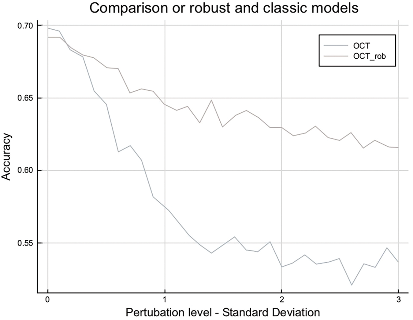
Figure 7: Robust logistic regression vs. standard performance

6.2 Robustifying the Training Set—OCT

We robustify the model by generating a training set that includes perturbed scenarios. We first select the three most important variables. We generate three additional training sets as shown in Fig. 8a, the first one where the three most important variables have been perturbed to a level of 0.5σ (in green), the second one to a level of σ (in orange), and the third one to a level of 1.5σ (in blue). We concatenate these three training sets with the initial one to build a final training set. Finally, we re-train the model on this concatenated set.

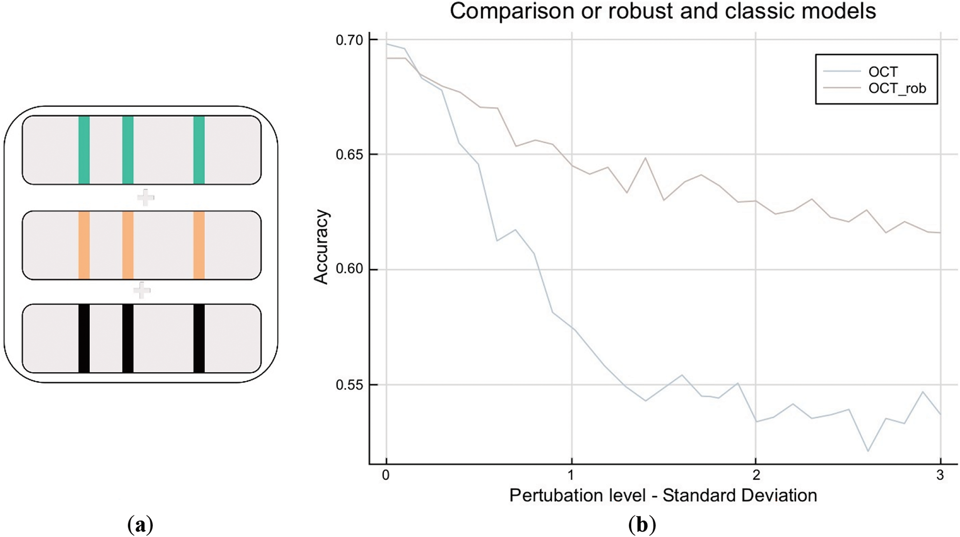
Figure 8: (a): OCT robustification: building the robust training set. (b): OCT robustification: robustification of training set

With an OCT of depth 5, there is a clear improvement due to robustification as shown in Fig. 8b. In highly perturbed scenarios, the accuracy stays at 0.62, whereas the non-robust model falls to 0.55. It is very interesting to observe that this comes at no cost for low perturbations, as both models stay at a level of 0.70. We also conclude that this model is far more robust than the regularized logistic regression as it maintains accuracy at a level of 0.60, whereas regularized logistic regression falls below 0.40. Lastly, in highly perturbed scenarios, the robust model remains accurate, similar to the baseline, while still predicting all three treatment classes as in Fig. 9. This represents an improvement as we can differentiate patients and prescribe less-invasive methods instead of the current practice, which prescribes high doses to all patients.

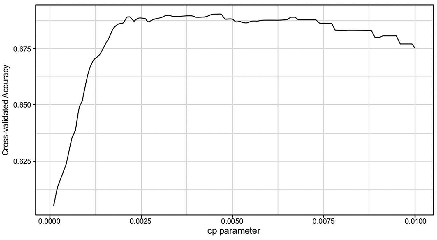
Figure 9: Cart cross-validation Cp parameter vs. accuracy

7  Conclusion

To conclude, this research had two major contributions. The first one is building models that allow us to predict the best treatment for a patient with accuracy levels of 0.70 (an improvement from 0.64 baselines). This personalized approach improved the previous practice of simply prescribing the most commonly effective treatment to all patients. We also note the three top features (i.e., the presence of any serious adverse effects), which are sufficient to make highly accurate predictions.

The second contribution is the robustification of the OCT model by designing a new training set. These include perturbed scenarios, and it is based on a sparse number of features (the three most important ones). The major observation is that it came at no cost in unperturbed scenarios while remaining much more robust in perturbed ones. These outperform models that are already robust, such as regularized multinomial logistic regression.

Nevertheless, this robustification design came at the cost of the interpretability of our models. We can associate a price to the interpretability of models as defined in the paper [17]. Interpretation is reduced since we train on a concatenated dataset that includes the same patient observation multiple times (with perturbations). An interesting area of research to explore is which price could be associated with this process and which formulation could be developed to include this price. For example, the interpretability penalty can be added as part of the mixed integer Optimization (MIO) formulation of an OCT or a regularized term in logistic regression.

Acknowledgement: We would like the acknowledge Laikipia University for availing the ICT environment and resources to conduct this research.

Funding Statement: The authors received no specific funding for this study.

Author Contributions: Gilbert Langat—conception, design, writing of the manuscript. Alex Kibet—analysis, interpretation, revision. All authors reviewed the results and approved the final version of the manuscript.

Availability of Data and Materials: Data that support the findings of this study are available upon reasonable request.

Ethics Approval: Not applicable.

Conflicts of Interest: The authors declare no conflicts of interest to report regarding the present study.

References

1. National multiple sclerosis society. [cited 2022 Dec 22]. Available from: https://www.nationalmssociety.org/What-is-MS/Who-Gets-MS. [Google Scholar]

2. Chalkou K, Steyerberg E, Egger M, Manca A, Pellegrini F, Salanti G. A two-stage prediction model for heterogeneous effects of many treatment options: application to drugs for Multiple Sclerosis. arXiv:2004.13464. 2020. [Google Scholar]

3. Kent DM, Steyerberg E, van Klaveren D. Personalized evidence based medicine: predictive approaches to heterogeneous treatment effects. BMJ. 2018;363:k4245. doi:10.1136/bmj.k4245. [Google Scholar] [PubMed] [CrossRef]

4. Kaur R, Chen Z, Motl R, Hernandez ME, Sowers R. Predicting multiple sclerosis from gait dynamics using an instrumented treadmill: a machine learning approach. IEEE Trans Biomed Eng. 2021;68(9):2666–77. doi:10.1109/TBME.2020.3048142. [Google Scholar] [PubMed] [CrossRef]

5. Ghasemi N, Razavi S, Nikzad E. Multiple sclerosis: pathogenesis, symptoms, diagnoses and cell-based therapy. Cell J. 2017;19(1):1–10. doi:10.22074/cellj.2016.4867. [Google Scholar] [PubMed] [CrossRef]

6. Goldenberg M. Multiple sclerosis review. Pharm Ther. 2012;37(3):175–84. [Google Scholar]

7. Tramacere I, Del Giovane C, Salanti G, D’Amico R, Filippini G. Immunomodulators and immunosuppressants for relapsing-remitting multiple sclerosis: a network meta-analysis [Internet]. Cochrane Database Syst Rev. 2015;9:CD011381. [cited 2022 Dec 22]. Available from: https://www.cochranelibrary.com/cdsr/doi/10.1002/14651858.CD011381.pub2/full. [Google Scholar]

8. Zelilidou SP, Tripoliti EE, Vlachos KI, Konitsiotis S, Fotiadis DI. Segmentation and volume quantification of MR Images for the detection and monitoring multiple sclerosis progression. In: 2022 44th Annual International Conference of the IEEE Engineering in Medicine & Biology Society (EMBC); 2022 Jul 11–15; Glasgow, UK. p. 4745–8. [Google Scholar]

9. Debray TP, Schuit E, Efthimiou O, Reitsma JB, Ioannidis JP, Salanti G, et al. An overview of methods for network meta-analysis using individual participant data: when do benefits arise? Stat Methods Med Res. 2018;27(5):1351–64. doi:10.1177/0962280216660741. [Google Scholar] [PubMed] [CrossRef]

10. Belias M, Rovers MM, Reitsma JB, Debray TPA, IntHout J. Statistical approaches to identify subgroups in a meta-analysis of individual participant data: a simulation study [Internet]. BMC Med Res Methodol. 2019;19:1–3. [cited 2022 Dec 22]. Available from: https://www.ncbi.nlm.nih.gov/pmc/articles/PMC6720416. [Google Scholar]

11. Caster O, Ralph Edwards I. Quantitative benefit-risk assessment of methylprednisolone in multiple sclerosis relapses. BMC Neurol. 2015;15(1):206. doi:10.1186/s12883-015-0450-x. [Google Scholar] [PubMed] [CrossRef]

12. Hanson G, Chitnis T, Williams MJ, Gan RW, Julian L, Mace K, et al. Generating real-world data from health records: design of a patient-centric study in multiple sclerosis using a commercial health records platform. JAMIA Open. 2022;5(1):110. doi:10.1093/jamiaopen/ooab110. [Google Scholar] [PubMed] [CrossRef]

13. D’Alisa S, Miscio G, Baudo S, Simone A, Tesio L, Mauro A. Depression is the main determinant of quality of life in multiple sclerosis: a classification-regression (CART) study. Disabil Rehabil. 2006;28(5):307–14. doi:10.1080/09638280500191753. [Google Scholar] [PubMed] [CrossRef]

14. Petzold A, de Boer JF, Schippling S, Vermersch P, Kardon R, Green A, et al. Optical coherence tomography in multiple sclerosis: a systematic review and meta-analysis. Lancet Neurol. 2010;9(9):921–32. doi:10.1016/S1474-4422(10)70168-X. [Google Scholar] [PubMed] [CrossRef]

15. Bertsimas D, Dunn J. Optimal classification trees. Mach Learn. 2017;106(7):1039–82. doi:10.1007/s10994-017-5633-9. [Google Scholar] [CrossRef]

16. Leist AK, Klee M, Kim JH, Rehkopf DH, Bordas SPA, Muniz-Terrera G, et al. Mapping of machine learning approaches for description, prediction, and causal inference in the social and health sciences. Sci Adv. 2022;8(42):1942. doi:10.1126/sciadv.abk1942. [Google Scholar] [PubMed] [CrossRef]

17. Bertsimas D, Delarue A, Jaillet P, Martin S. The price of interpretability. arXiv:1907.03419. 2019. [Google Scholar]