Geometric Morphometrics Applied to Cartography

1  Introduction

The shape is analyzed in cartography in two different ways by statistical methods. The first one consists in analyzing the intrinsic shape of objects, in particular by calculating specific indices (Gravelius compactness index, Miller circularity index, elongation index, concavity index, etc.) or even by fractal geometry. Another way consists in considering the morphology of a background map not for itself but by comparison with that of another base map. In this case, it is a question of measuring the morphological difference between the two objects. This can be revealed by a cartographic transformation moving the points, lines and polygons making up the background map [1,2]. The general underlying hypothesis, resulting from the work of the naturalist D’Arcy Thompson1 [3] is the following: “The shape expresses the structure of a phenomenon; if one can characterize a shape or to compare shapes, then one can reveal through the form an invisible structure, one can compare structures with each other” [4]. Geographic maps, as representations of a specific space, are structured by landmarks (in particular places) separated from each other according to a measure of distance. However, for the same space, these distances can vary, for example between ancient maps, between cognitive representations of this space or even between maps expressing the distance in travel time. Comparing the shape of these maps reveals their hidden structure and shows the differences in the measurement of these distances. The method and the software presented in this article, adopt this second approach to compare the shape of several geographical maps. Kendall [5] defined shape as “the residual geometric information of an object once its size, position and orientation have been filtered out”. The shape is therefore distinguished from the form, in particular by Needham’s equation [6]: “Form = shape + size”. Analyzing the form therefore means considering the size of the object, i.e., not filtering it (or reintroducing it) in the analysis, which can be relevant for morphometric studies of biological organisms but which is of little interest for geographical maps. They will therefore be compared here by their shape.

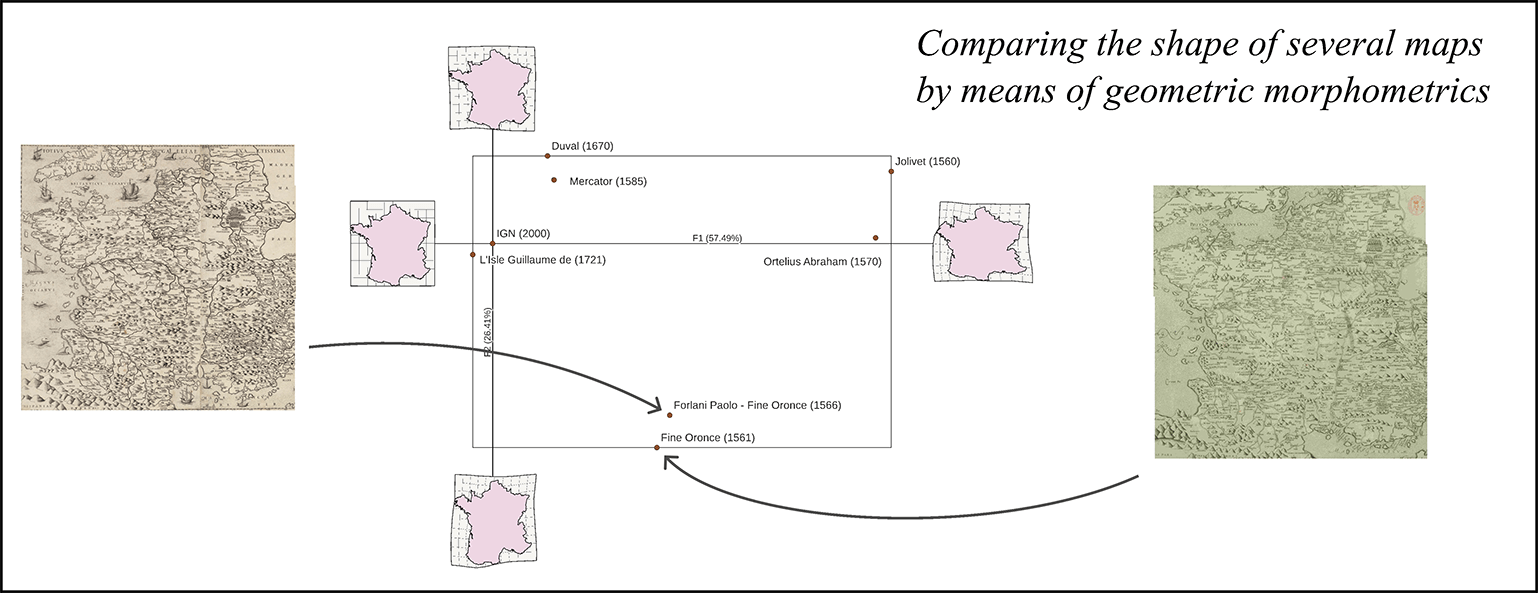
Bidimensional regression [7,8] has been the most used method in cartography since the 1970s to compare the shape of two maps, by filtering out the geometric data unrelated to this shape. Waldo Tobler’s method is based on the comparison of the relative position of homologous landmarks corresponding to each other on an image map and a reference map. The image landmarks can correspond, for example, to those drawn on a sketch map externalizing the cognitive representation of a particular space or to those of an ancient map. The bidimensional regression method is composed of two successive steps. The first is an adjustment of all the landmarks of the image surface to be analyzed on those of the reference surface, a topographic map for example. This adjustment is an adaptation of the simple linear regression to bidimensional data. When the compared surfaces are geographical maps, the landmarks in question correspond to places, i.e., elementary portions of the geographical space, identified by a toponym. The image landmarks are moved so that they are located as close as possible (in the sense of least squares) to their counterparts on the reference surface. After the adjustment, the size, position and orientation of the coordinates have indeed been filtered and the remaining geometric information corresponds well to the shape. The second step is an interpolation of cartographic data. The residual differences between the image and reference coordinates are used to deform the reference surface by an interpolation calculated from the displacement vectors corresponding to each pair of homologous landmarks. The result of this cartographic transformation of position is a cartographic anamorphosis, more precisely a polycentric distance cartogram capable of revealing the invisible underlying structure of the image map. The figure below presents an example in the field of ancient maps (Fig. 1).

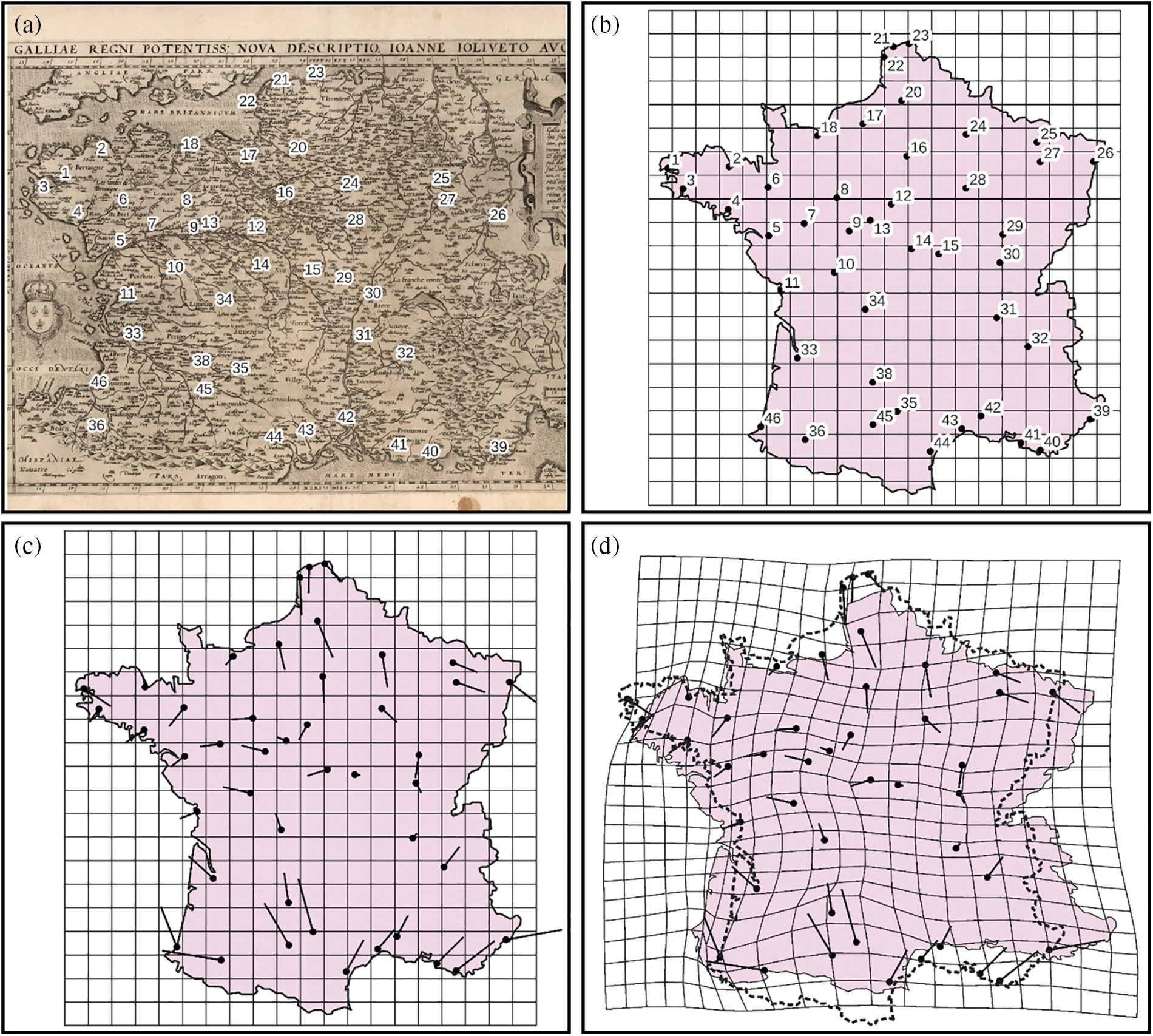
Figure 1: Comparison of the shape of two maps by bidimensional regression: the cartography of France by Abraham Ortelius (1570) is compared to a modern Map (source: gallica.bnt.fr/National Library of France). (a) The vectorized sketch of 44 cities from the ancient map. (b) The modern reference map with its 44 homologous landmarks used for the morphological comparison. (c) Step 1: adjustment by the bidimensional regression. The image landmarks of the ancient map are moved closer to the reference landmarks. The displacement vectors correspond to the residual displacement between each pair of homologous landmarks. (d) Step 2: the grid and the contour of France have been deformed according to the displacement vectors

However, bidimensional regression can only compare two maps at a time. To overcome this limit, we associate the regression fit with a method of standardization fit derived from the natural sciences and used to compare the shapes of several objects, also from homologous landmarks: geometric morphometrics [9–11]. Bookstein [12] defined this new morphometric approach as the statistical analysis of variations in shapes and their covariations with other variables. Baab et al. specified that the objectives of geometric morphometrics refer to three main categories: to characterize and quantify the main directions of variations and covariations of shapes in a sample; test whether two or more groups differ in certain aspects of the shapes; establish the nature of the relationship between the shapes and one or more additional variables [13].

Bidimensional regression and geometric morphometrics seem to us sufficiently close in their methodology to associate them in the same cartographic software. Regularities, similarities, and dissimilarities of cartographic shapes can be detected and cross-checked with other indicators. Several software have been developed since the 90s for geometric morphometrics. These include, without being exhaustive, IMP [14], Morphologika [15], MorphoJ [16], the R package Geomorph [17], and the series of tps software [18]. These software programs are all capable of performing geometric morphometric analyzes from maps but cannot read cartographic file formats such as the shapefile format used by the MapMorphy software presented in this article. This file format allows existing cartographic data (e.g., illustrations) to be directly integrated into data processing and can be easily produced (e.g., image landmarks) by GIS tools used by cartographers. Likewise, all vector files produced by MapMorphy can be formatted using GIS software.

2  Some Examples of Potential Applications of Geometric Morphometrics in Cartography

Geometric morphometrics has already been used in many fields of research (biology, archaeology, botany, image analysis, chemistry, medicine, bioinformatics, genetics, geology, etc.). The first applications relating to cartography concern spatial analysis. They were carried out by statisticians to test Christaller’s theory of central places [19]. Mardia et al. [20] verified this hypothesis for a map of 44 cities in the state of Iowa (USA) in the seventies. They compared the shape of the polygons resulting from a Delaunay triangulation between triplets of nearby cities with the equilateral triangles of the theoretical situation. The question was whether the proportion of nearly equilateral triangles between cities was more important than a random distribution. Kendall [21] also found a higher-than-expected proportion of equilateral triangles corresponding to the distribution of 234 cities and towns in Wisconsin. More recently, geometric morphometrics has been applied to human traces on the ground, such as footprints [22] or constructions such as Neolithic dwelling plans [23]. For a comprehensive review of applications, see Mitteroecker et al. [11].

All these structures (human traces or others) can of course be the subject of a map when they are located in a geographical reference frame, especially because geometric morphometrics analysis produces shape variables for each object. But the map, as a direct object of this method, is not a topic that has been explored to date. We propose to explore this approach as the extension to several objects of the applications already practiced for the morphological comparison of two maps from bidimensional regression. It will therefore be a question of comparing the shape of several image maps to the shape of a single reference map. The first possible category concerns the comparison of maps resulting from the measurements of the terrestrial space carried out in conventional systems of coordinates and units of distance. The cartographic shapes can indeed vary according to the methods and techniques used over time, from the astrolabe to the satellite, including the land surveyor’s chain and triangulation. These shapes could be analyzed from the perspective of the level of precision between ancient and modern maps [8] (Fig. 1), but also between modern maps using different technologies [24]. The analysis of cartographic shapes also makes it possible to better understand the context of the elaboration of ancient maps of which we often know little. Many of these maps were based on previous productions. By their shape, they provide information on their parentage, lineage, and even plagiarism [25].

But geographic space is not measured only with Euclidean distances expressed in meters or kilometers. Other possible cartographic applications in geometric morphometrics imply that there are other metrics, and that geographical space is not a neutral, unique and intangible container but that it is relative, that is to say, that it is constructed by the values associated with places. From this point of view, several non-Euclidean metrics can be superimposed and the exposed method makes it possible to compare the morphology of the resulting spaces in two registers. The first one concerns functional spaces [26]. On a daily basis, we evaluate what separates or brings places together according to values that are not measured in miles or kilometers. The physical space, objectified by universal metrics, is then replaced by a space where the layout of places is modified according to the functions assigned to them and the relationships attributed to them. For such spaces, distances in meters are replaced by effort-distances (time-distances, cost-distances, energy-distances, tiredness-distances, etc.) or by metaphorical distances measured, for example, by the number of social contacts between places (cultural exchanges, phone calls, etc.). The heterogeneous and anisotropic nature of these spaces can be visualized by a polycentric distance cartogram [27,28]. Geometric morphometrics makes it possible to simultaneously compare the shapes of several of these non-Euclidean maps, i.e., several time-space maps. The second register concerns cognitive spaces. Cognitive space corresponds to a functional space recognized by a subject [29,30]. The cognitive space therefore introduces an additional variation compared to the functional spaces because many individual factors such as motivation or personal characteristics come into play [29]. It produces in us a cognitive representation of space whose structure may be very different from that of “objective” space. Here again, the cognitive space can be revealed in the form of a polycentric distance cartogram [31,32]. A morpho-geometric analysis could detect constants in the transformation of space for groups of individuals and highlight cognitive spaces that are similar or opposite in shape.

3  Theoretical and Methodological Framework of the Implemented Method

3.1 Emergence of Geometric Morphometrics

From the 1960s and 1970s, what is now called traditional morphometrics [33] applied multivariate statistical methods (principal component analyses, discriminant analyses, etc.) to a set of measurements (linear distances, angles, surfaces, lengths, perimeters, etc.) or ratios [34,35]. However, this approach to comparative morphology does not make it possible to understand pure shapes because the analyzed linear measurements are usually strongly correlated with size. Several solutions have sought to eliminate the size effect, but with different results and none of them being unanimous [36]. From the end of the 80s, a new current of research emerged to characterize shapes by variables independent of size. These methods use all the Cartesian coordinates of a series of homologous identified points called landmarks or calculated points (semilandmarks) on each object [37–39], and no longer measurements between certain reference points. Several approaches have been used (Bookstein coordinates, Euclidean Distance Matrix Analysis, resistant fit, etc.) but it is the Generalized Procrustes Analysis (GPA) that has prevailed since the 1990s [40–42]. This method removes what is not about the shape by a translation, followed by a scaling and then a rotation of the coordinates [37,43]. Concomitantly, several statisticians and in particular Kendall [44,45] and Goodall [46,47] developed a statistical framework, a theory, for the statistical analysis of shapes including the fit of Cartesian coordinates and the obtaining of shape variables. Geometric morphometrics emerged in the 1980s from this convergence. It was a new current of research that some do not hesitate to describe as revolutionary [33,48]. In addition, to better visualize the differences in shape, geometric morphometrics uses, like bidimensional regression, a grid interpolation method in the spirit of the pioneering work of D’Arcy Thompson at the beginning of the 20th century, recently republished [3]. This is the so-called thin-plate splines method [49] which is generally applied to grids.

3.2 From the Configuration Space to the Shape Space

Shape differences appear through the exploration of a morphological space (also called morphospace). Its construction involves a series of operations on the initial coordinates of homologous landmarks. Initially, there is the configuration space. The configurations correspond to the coordinates of homologous landmarks including information on the position, the orientation and the size of several objects. The configuration space is the set of matrices of k homologous landmarks with M coordinate dimensions (2 or 3). The configuration space is potentially very large and therefore practically impossible to represent by the mind. Each configuration of K landmarks in M dimensions can be considered as a point in a space of K * M dimensions [50]. Thus, geographical maps structured by configurations composed of 20 places in 2 dimensions originally sit in a 40-dimensional configuration space. Statistically, such a space has 40 degrees of freedom because there are 40 independent pieces of information. To obtain a shape, it is possible to superimpose two configurations of landmarks by the ordinary Procrustes method [51]. The first step in this method is to center the two configurations relative to each other (removal of positional differences). The second step reduces them to size 1 thanks to the centroid size (removal of size differences). Centroid Size (CS) is the most commonly used measure of size in geometric morphometrics. It corresponds to the square root of the sum of the square distances between each landmark and the centroid of the configuration. This can be expressed as:

CS=∑i=1n(ui−x¯)2+(vi−y¯)2(1)

where u, v correspond to the coordinates of the configuration; x¯, y¯ correspond to the coordinates of the centroid of the configuration, and n the number of landmarks of the configuration.

To standardize the size of an object at the value of 1, it suffices to divide the coordinates of its homologous landmarks by the centroid size; finally, a rotation of one of the configurations on the other is carried out in such a way as to reduce the distance between the two configurations as much as possible (removal of orientation differences). This distance, called the Procrustes distance, corresponds to the square root of the sum of the square distances between each homologous landmark (Fig. 2). The Procrustes distance is therefore a measure of the difference between shapes. The greater this distance, the greater the differences in shape. Conversely, this distance is zero for two strictly identical shapes.

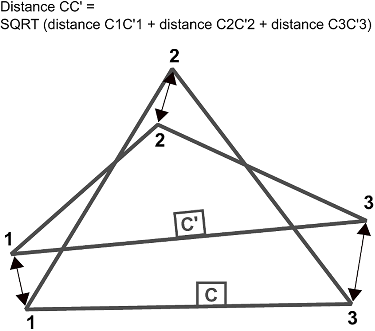
Figure 2: Calculation of the Euclidean Procrustes distance between two triangle configurations

Kendall [44,45] demonstrated that the shape space corresponding to the Procrustes metric is a riemannian manifold (curved space) of dimension 2K-4 for two-dimensional configurations. Indeed, the superposition reduces the number of dimensions, that is to say, the degree of freedom of the values. For 2D configurations, the shape space is reduced by four dimensions: two dimensions for position, one dimension for scaling and one dimension for orientation. These data are no longer necessary since they are common to the different configurations (same size, same position and same orientation of the homologous landmarks). The result is an isotropic (uniform) hyperspherical space in which each configuration is represented by a point separated from the others by a constant metric corresponding to the Procrustes distance.

By using the ordinary Procrustes method previously described, it is thus possible to visualize a space corresponding to shapes composed of three homologous landmarks [52,53]. The points corresponding to triangles then sit on a surface in 2 dimensions (2 dimensions * 3 landmarks − 4 dimensions). More precisely, Kendall’s shape space for triangles corresponds to the 2D surface of a 3D sphere of radius of 0.5. The table of Procrustes distances between pairs of configurations then makes it possible to produce Kendall’s shape space for triangles, for example by means of MDS (multidimensional scaling). For more than three landmarks, Kendall’s shape space corresponds to a hypersphere of dimension greater than 3 (Fig. 3).

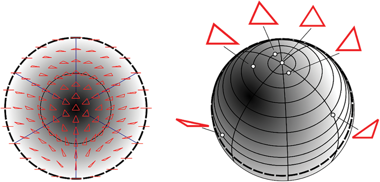
Figure 3: Kendall’s shape space for triangles (after Klingenberg [54]). In such a space, each triangle corresponds to a point on the sphere and the distances between points correspond to the differences in shape (distances on the arc or in a straight line). If an equilateral triangle is chosen as the North Pole, then several regularities emerge: to the South Pole corresponds to another equilateral triangle and the content of the Southern Hemisphere is the symmetrical of that of the Northern Hemisphere. At the equator (thick dashes), correspond to the flattened triangles while at the meridians correspond to the isosceles triangles

Current work in geometric morphometrics is based on that of Kendall. However, they most often use a generalized version of Procrustes fit: GPA, Generalized Procrustes Analysis [9,37,43]. It was indeed suggested by Rohlf [38] that when data from curved space are projected onto a tangent linear space for statistical analysis (see below), distances between objects were better respected when the shape space was produced from the GPA [55]. Several properties distinguish the GPA shape space (sometimes called the Slice shape space) from the Kendall shape space. 1. The fit is no longer applied there between the homologous landmarks of each pair of configurations but between the homologous landmarks of each object and those of a unique reference. 2. This unique reference ideally corresponds to the average of the Procrustes-fitted coordinates and is called consensus in this case. Consensus is calculated during the iterative process of fitting. An external reference to the images can also be chosen however the risk of a lower quality of the model. 3. Depending on how the size is processed during this iterative adjustment, the GPA produces two kinds of shape space, each endowed with a specific metric [50,53,56]. When size is neutralized by standardizing all objects to a centroid size of 1, the fit is said to be partial. When the size is constrained to the value of 1 for only one object and it can vary to reduce the Procrustes distance of the others, the fit is said to be full. 4. When a partial generalized fit is used (which is the most frequent case), the shape space does not correspond to a sphere but to a hemisphere (for triangles) or a hyper-hemisphere (for more than three homologous landmarks) of radius of 1. It has been shown that there is a relation between Kendall’s shape space and the Slice shape space produced by partial generalized fitting [55]. For more details on shape spaces and related metrics, see the article by Klingenberg [53].

3.3 From the Shape Space to the Morphospace

In order to visualize and explore the shape space, a reduction in the number of dimensions is necessary. It is possible to do this by using a multidimensional analysis of the data to produce a relevant perspective on the shape space, which we will call here morphospace. However, the shape space is a curved space that does not lend itself well to linear statistical methods such as principal component analysis. On the other hand, when the individuals are grouped on a relatively limited portion of the curved space, which is the case after the fit, we can project their coordinates with little deformation on a linear tangent space whose point of contact with the curved space corresponds to the reference configuration (Fig. 4a), ideally the consensus [57]. The tangent space is then of the same dimension as the curved space. The problem is comparable to that of cartographic projections which seek to convert the angular geodesic coordinates into Cartesian coordinates on a tangent plane: the closer the individuals are to the point of tangency on the curved space, the more faithful will be their projection on the tangent space. The most used method in geometric morphometrics is an orthogonal projection during which the coordinates of the homologous landmarks are projected perpendicular to a space which is tangent to the point of reference2 [38].

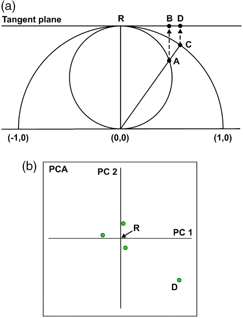
Figure 4: From the shape space to the morphospace (an example with triangles). (a) Sectional view of the articulation of Kendall’s shape space for triangles (the sphere of radius of 0.5), the shape space by fitting to a reference (hemisphere of radius of 1) and the tangent space (the horizontal plane). The three spaces have a common point: the reference R. Point A corresponds to the position of a triangle on the sphere (full superimposition with a size closest to that of R) and B, its orthogonal projection on the tangent plane. C corresponds to the same fitted triangle but is reduced to centroid size of 1 and D its projection on the tangent plane (after Klingenberg [54]). (b) A morphospace corresponds to the visualization of the individuals in the tangent plane according to two or three of the first components of a principal component analysis

A principal component analysis can then be applied to the projected coordinates of the individuals on this tangent space. In geometric morphometrics, the advantage of PCA over other multidimensional data analysis methods is that it operates a rigid rotation of the data on the main axes (those with the greatest variances) while preserving the original distances [50]. Principal component analysis [9,12] and its equivalents such as relative warp analysis [58] have thus become central tools for analyzing geometric morphometrics data to show the essential morphological differences [59–61]. The first use of PCA is to show a morphospace generally built from the first two components in which each individual represented by a point is separated from the others by distances which approximate that of the multidimensional shape space (Fig. 4b). It is therefore easy to evaluate the resemblance of two maps or on the contrary their dissimilarity by their location in this space. In addition, PCA eigenvectors can be used to compute models for any point of the morphospace. Finally, the scores of the individuals (e.g., geographical maps) on the axes can be considered as shape variables that can be cross-referenced with other data. In order to construct the morphospace, the coordinates of the reference are subtracted from those of each adjusted object, which has the effect of centering the morphospace on this reference. The PCA is then calculated from the covariance matrix of these residuals. The principal components then constitute linear combinations of the original data which are independent of each other. The eigenvalues describe the decreasing percentage of variance that is explained by each axis. The scores of the principal components correspond to the position of each object, therefore of each map, along the axes. The first axis corresponds to the main tendency of variation of shapes, the second axis, to the second in terms of importance, etc. The orthogonal crossing of two or three of these axes therefore makes it possible to represent a morphospace in which each map is arranged according to the main shape variations. For more than three homologous landmarks, keep in mind that this is a partial view of the shape space.

4  The MapMorphy Software

The MapMorphy software was designed to implement the methods previously described and allow the user to compare the morphology of several surfaces structured by homologous landmarks, in particular geographical maps. The application uses the open-source MapWinGIS ActivX (https://www.mapwindow.org/), a software component that brings all the functionalities of a geographic information system to MapWindow GIS. MapMorphy was developed in the VB.net language and the Microsoft™ company Visual Studio Community integrated development environment. Supplementary materials are available at: https://mapmorphy.fr. They include the MapMorphy installer, documentation, and examples.

4.1 Input Data

The software user begins by choosing the data files necessary for processing. All should be coded in shapefile3 format. The main data correspond to the homologous landmarks. These are identifiable points, precisely localizable on each of the objects of the studied corpus, which are present both on all the image maps and on the reference map. These landmarks must meet several requirements [62]. They must first of all make it possible to summarize the morphology of each object and must therefore be correctly distributed on its surface and sufficiently numerous. When a hypothesis concerns one or more landmarks, these must necessarily be part of the input data. The landmarks must be digitized precisely or according to a particular convention if maps present ambiguities regarding their location (for example on ancient maps). Finally, landmarks must maintain between them a relatively similar topology for the method to be convincing (cf. 4.4). For structures relating to living things, the statistician and biologist Bookstein classify landmarks into three types with decreasing level of homology. It is striking to note for a geographer that for this author, landmarks are comparable to places, as if this geographical concept best defined the notion of landmark from a general point of view: “These are loci that have names (‘bridge of the nose’, ‘tip of the chin’) as well as Cartesian coordinates” [12]. Conversely, by its properties, the place (or locus) appears from a geographical point of view as a concept perfectly adapted to the notion of landmarks in the sense of geometric morphometrics. First of all, answering the question “where”, the place has spatial properties: it is located in a unique way, possibly in a Cartesian coordinate system, by its projected geographical coordinates. It is indivisible and mathematically discrete. It can be isolated, occupies a well-determined surface and can exist at all scales, from the micro-place like a square or a church, to the macro-place like a country. In addition, the place has social characteristics that make it a very unique landmark. The place only exists through the meaning attributed to it. “An expanse only becomes a place at the end of a process of mental construction which individualizes it in relation to the surrounding space and which is based on individual or collective practices and experiences” [63]. The place must therefore be recognized by some or by all for its qualities, its functionalities, its appearance in order to be consecrated as a place. As such, it has an identity expressed by a toponym. For all these reasons, the place can be assimilated to a type 1 landmark in Bookstein’s typology, those presenting the strongest homology. Other secondary data can be added to the project, optionally. When an external reference is chosen (for example a topological map), it is possible to add to it illustrative plots of points, polylines or polygons which will be deformed with a grid during the interpolation process, according to the differences observed between fitted landmarks and reference landmarks. If the consensus is chosen as a reference, it is possible to associate link files connecting the fitted landmarks, in the absence of illustrations. In addition, bitmap files from photographs or scans of the compared objects can be added to the project. Due to the privileged geomatics format of the data, the software is specially adapted to the comparison of geographical data. It is however able to compare any corpus of surfaces structured by a series of homologous landmarks coded in shapefile format.

4.2 A GIS User Interface

MapMorphy has a graphical user interface (GUI). It offers two different aspects corresponding to two distinct but complementary types of projects (Fig. 5).

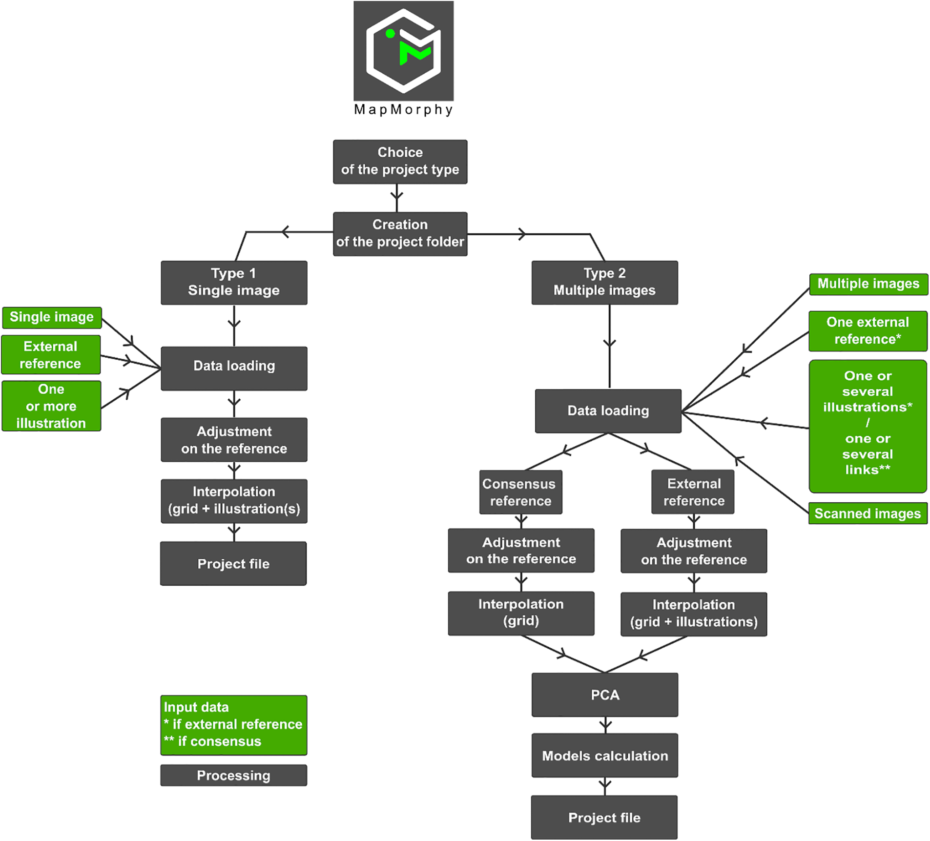
Figure 5: Simplified processing of both types of projects in the MapMorphy software

The type 1 project corresponds to the comparison of a single image configuration with a reference configuration. This type of project computes a classical polycentric cartographic transformation of position by ordinary bidimensional regression [8,64]. It can be displayed by a polycentric distance cartogram. The processing menu is used to launch the two successive stages of a bidimensional regression as described above. The first step is a superimposition of the image landmarks of a configuration on the reference landmarks. The residual differences (there are always some if the two configurations are not strictly identical) determine the displacement vectors for each landmark of the reference configuration. The user interface then proposes to define the extent and the resolution of a grid which covers the reference space and represents a continuous space. The second step is a configurable multiquadric interpolation which allows to propagate all the deformations corresponding to the displacement vectors on the grid and the illustrations relating to the reference map. The cartogram then appears in the principal window. This type of project makes it possible to show the difference in shape between the landmarks of an image configuration with those of a reference topographic map (Fig. 1) or to compare an average of image landmarks of a configuration with the topographic landmarks of this reference. It is complementary to type 2 projects.

The type 2 project corresponds to the morpho-geometric analysis of the software. It presents an additional visualization panel for the exploration of the morphospace. This time, it is a matter of comparing several image configurations to a reference configuration, and this, in four steps. The first two are the same as type 1 projects, except that the reference can match the consensus or an external reference and the data can be projected onto a tangent plane. If the consensus is chosen as the reference, no illustration is available, because the consensus is an average that does not correspond to any possible illustration. However, links between the superimposed adjusted landmarks provide additional visual context to the interpolated grid. These first two steps make it possible to calculate, show and save the total difference in shape between each map and the reference map. This difference can then be visually compared to the partial reconstruction by the model. The third step calculates the PCA and the morphospace. The PCA is constructed from the covariance matrix of superimposition residuals. The PCA of MapMorphy makes it possible to reconstruct, for any point and thanks to its eigenvectors, typical models, four of which are displayed on the PCA graph. An additional window allows to calculate a model for each point of this continuous morphospace. This window also makes it possible to evaluate, by a linear regression test, the relevance of the data for a morpho-geometric analysis (cf. 4.4). Finally, the fourth step, associated with the calculation of the PCA, is an unsupervised classification by K-means witch allow to associate the close shapes on the PCA.

Both interfaces are very similar. The type 1 interface is a simplification of the type 2 interface, so many tools and visual codes are common to both types of projects. The user interface uses the standard presentation of GIS software for cartographic navigation, management of data layers, attribute table, identification of objects, formatting. The two types of project are processed according to comparable sequences: choice of the project type, creation of the project folder, loading of necessary and optional data, superimposition and creation of the grid, multiquadric interpolation, PCA associated with the clusters (only for type 2 projects). In both cases, all processing is automatically saved in the folder previously designated by the user. This folder contains the vectors and attribute data in shapefile format and the statistical results in text format (which can be consulted in the software). At the end of processing, the project file is saved in this folder with the relative paths to the folder. This project file redisplays the data layers, dispensing with reloading them and recalculating the graphical and statistical processing.

MapMorphy makes it easy to view and interact with the map dataset. The selection of a geographical map in the morphospace entails, for example, the visualization of its total difference in shape with the reference. The Model can then be displayed and the corresponding variables can be consulted in an attribute table and a floating identification window. Additional analyzes and formatting can be carried out in other software from the produced results saved in the project folder. The individuals in the morphospace can be thus easily joined with a geographical location in a GIS thanks to the shapefile format. Figures 6 and 7 show an example based on ancient maps.

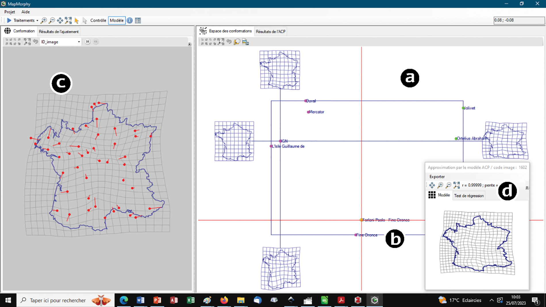
Figure 6: MapMorphy user interface for a type 2 project. This test is only intended as an illustration of the presented method. The shape of seven ancient maps of France4 structured by 44 homologous landmarks is compared to a modern map named IGN at the intersection of the axes. The reference here is not the consensus but external data which could therefore be associated with an illustration corresponding to the modern limits of the country. The linear regression test (Fig. 8b) nevertheless reveals that the data can be processed by PCA without recourse to consensus and that the model is reliable. (a) The morphospace corresponds to the scores on the first two components of the PCA which cumulate nearly 84% of the variance. The proximity of the points brings to light the proximity of the shapes. Four typical models are displayed at the ends of each axis (PC1 on the horizontal axis and PC2 on the vertical axis). They correspond to the points of intersection of the rectangular frame with the two axes and show the two main trends in shape deviation from the reference. (b) For example, the map of Paolo Forlani and Oronce Fine (1566) is targeted by the user (red cross). Its similarity in shape with the previous map of Oronce Fine (1561) is highlighted here by the software. (c) Its total deviation from shape with the reference is displayed in the left window. (d) Its reconstruction by the model using the first two PCA components is displayed in the floating window

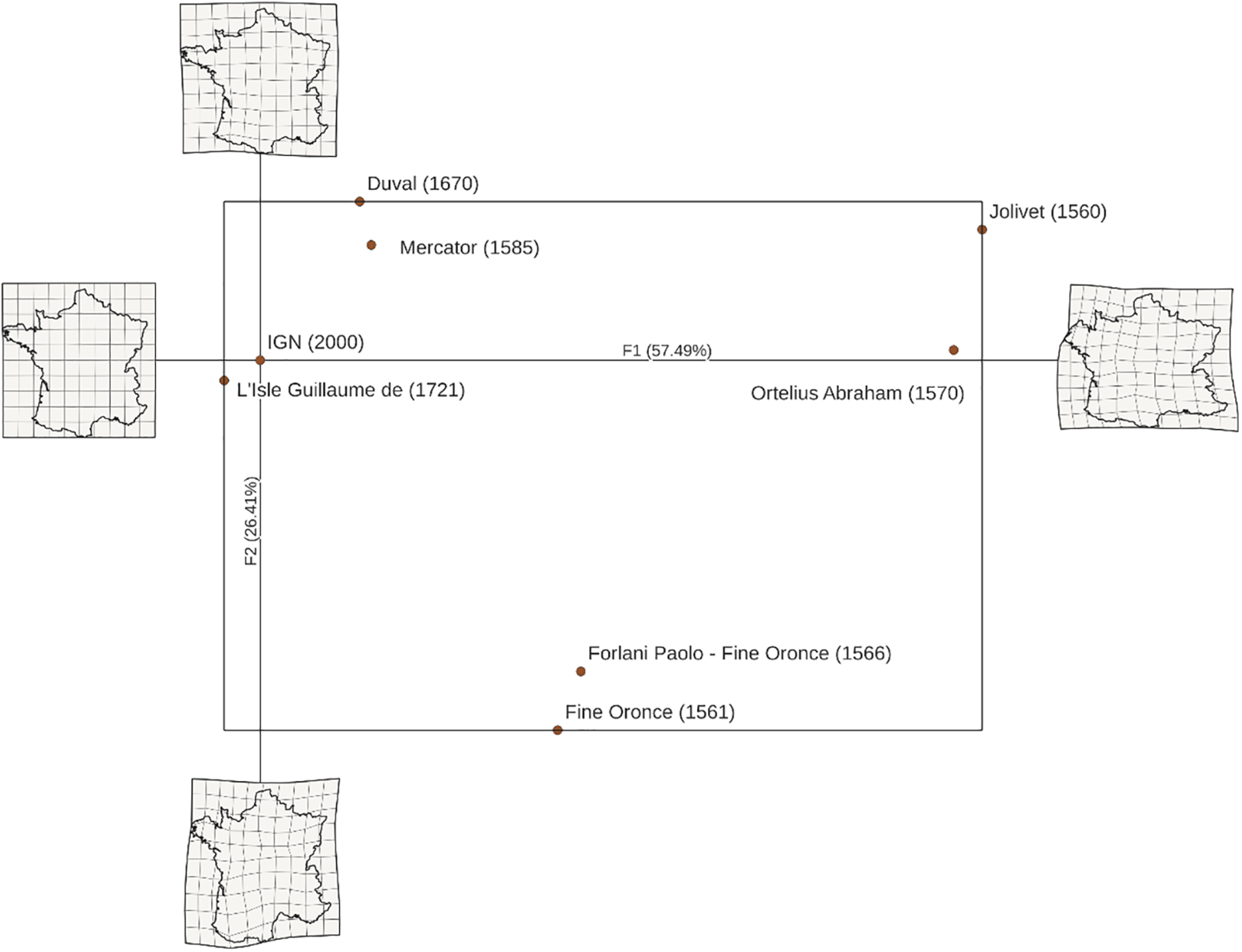
Figure 7: Vector formatting of the morphospace from files calculated by MapMorphy

4.3 Construction of the Shape Space Centered on the Consensus

The statistical adjustment method occupies a central place in the software for the construction of the shape space and therefore that of the morphospace. MapMorphy uses bidimensional regression, classically used in geography to compare two surfaces and is considered equivalent to the ordinary Procrustes method [65]. It is therefore used as it is in type 1 projects which only compare two sets of landmarks. By consistency, bidimensional regression is also used to construct, with an adaptation, the shape space of type 2 projects which compare several images. We present here the iterative process of optimal adjustment, that is to say the one using consensus as a reference. At the end of the generalized fitting, each point in the shape space corresponds to a specific shape and each particular shape corresponds to a point in the shape space. The adjustment method chosen for the software is of the partial type, so the size of all the configurations will be reduced to the value of 1 during the following process:

1.    Calculation of the centroid of each configuration.

2.    Calculation of the centroid size of each configuration as previously described (Eq. (1)).

3.    Calculation of the centered coordinates reduced to value of 1 of each configuration.

4.    Choice of the first centered-reduced configuration as provisional consensus.

5.    Rotation of the coordinates of all the configurations as close as possible to the consensus. The bidimensional regression calculation has been modified to simply pivot the data.

6.    Calculation of the new consensus (average of the coordinates of the shapes).

7.    Calculation of the average distance between the shapes and the new consensus (distances are calculated as in Fig. 2).

8.    Back to 5 until this average distance stabilizes.

At the end of this iterative process, we obtain the adjusted coordinates of all the original configurations and those of a consensus, that is to say of an optimal reference. These coordinates are used to create links between landmarks from a diagram provided with the data loading. They can then be projected onto a tangent plane and used in PCA to construct the morphospace.

4.4 Testing the Validity of the Cartographic Data

The process of recursive adjustment on the consensus aims to reduce the distance between all the shapes and the reference as much as possible so that the points corresponding to each individual are located on the smallest possible part of the shapes space. The consensus is the best-suited reference for this objective because it allows all shapes to be grouped together as closely as possible after the fitting process. As in the natural sciences, however, it is possible to use a reference other than the consensus [66,67], i.e., a topographic map. In this case, the difference between the reference and another shape can then be interpreted as a transformation not only mathematical but also geographical. However, the difference between the shapes and this reference will be greater than with the consensus and the calculation of the models will possibly be less efficient. Because distances between shapes must be small enough for modeling, geometric morphometrics should be used on objects with relative morphological resemblance. When analyzed shapes are related, data is indeed very close to the projection point (the reference) and there are not too many differences between data in the curved shape space and those in the linear tangent space. This is particularly the case for the usual objects of geometric morphometrics, that is to say mainly biological structures. On the other hand, when too large differences remain between all the shapes, image points are less grouped around the reference in the shape space. The points corresponding to the individuals are further away from the point of tangency and the approximation in the tangent space is distorted with respect to the curved space (Fig. 8a). This may be the case for certain geographical data, in particular for cognitive spaces having physical space as a common reference but constructed by individuals with necessarily very different individual characteristics and experiences [29,30].

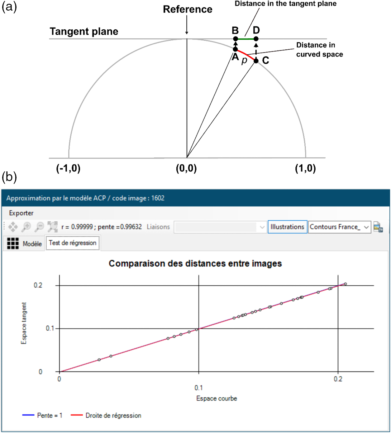
Figure 8: Are shape variations small enough for statistical analysis of tangent space? (a) The two distances compared (example with triangles). The distance A–C is the geodesic Procrustes distance p on the curve. B and D correspond to the location on the tangent space (here a plane) of the projection of points A and C, respectively. The Euclidean Procrustes distance B–D constitutes the second distance. It is calculated as indicated above (Fig. 2) but with the projected coordinates. The more the points deviate from the point of tangency R, the less these two distances correspond as on a cartographic projection (see also Fig. 4). (b) The graph under MapMorphy of the linear regression relating each pair of distances calculated for the individuals (the test concerns the data of Figs. 6 and 7). Only half of the distance matrix is considered for the calculation of the linear regression (distance A–C = distance C–A and distance B–D = distance D–B). The points must be globally aligned for the results of the PCA and the modeling to be relevant. The blue line has a slope of 1. The red line corresponds to the regression model and should ideally overlap and hide the blue line as in the case presented here

This is why MapMorphy includes a tool5 to test the relevance of a statistical analysis of tangent space coordinates (Fig. 8b). Using a linear regression through the origin, the software compares all the distances between pairs of individuals in curved space (geodesic Procrustes distance in radians) and in tangent space (Euclidean Procrustes distance). When shape variations are small between individuals, i.e., when the points corresponding to the objects are close to the point of tangency in the shape space, these two distances evolve together and the regression data are aligned. In this case, statistical analysis on the tangent space can be carried out without fear because the tangent space correctly represents the distances of the curved space. When significant differences between individuals are observed, it is therefore advisable to eliminate the outliers by deleting the configurations presenting excessive variations (for example from the RMSEs calculated by MapMorphy). This modifies the morphospace, and improves the quality of the modeling and the results of the linear regression test.

5  Conclusion

Geometric morphometrics is a powerful method for comparing the morphology of several structures and therefore of several maps. But like any method, it must be applied within a framework and on specific data (homologous landmarks, related shapes, etc.). We have developed the MapMorphy software to easily apply this method to cartographic data.

MapMorphy relies on the functions of the Morphoses plugin for MapWindow GIS (https://www.morphoses.eu/). This extension was intended to calculate by bidimensional regression and in a single pass, several adjustments on the same reference. The objective was then to express the shape of the average cognitive space in a group of individuals with a specific profile (age, sex, location, etc.). MapMorphy's morphogeometric method is significantly different from its predecessor since it is no longer a question of calculating an average shape from an a priori on the profile of individuals but of comparing shapes and exploring the profile of individuals with similar shapes6.

MapMorphy is a hybrid software combining bidimensional regression and the main principles of geometric morphometrics. In fact, the software no longer limits its objectives to spatial cognition but extends them to all surfaces structured by homologous landmarks, including biological structures. The specificity of the software remains however to process geographical data like ancient maps for example. In this case, it will be necessary to verify that the level of variation of the data is sufficiently low to be able to consider that the coordinates of the tangent space constitute a representative approximation of the data of the shape space. This condition is most often fulfilled in the natural sciences but not necessarily for geographical data. In addition, the software compares the variations of the shapes from a global point of view, because all the homologous landmarks are moved during the adjustment. The method is therefore not suitable for analyzing the variation of a particular place in the sample.

The current limits of the software concern the absence of statistical methods allowing to cross the shape variables (the scores on the PCA) with other variables. However, this can be done by other software from the saved results. In addition, the page layouts and vector formatting must also be produced by other software, for example, GIS software, from files in shapefile format produced during the automatic processing. The objective is now to be able to take semilandmarks into account, which would make it possible to extend the field of action of the software to structures delimited by curves and no longer only by landmarks. In the end, MapMorphy is presented as a software calculating the basic operations of geometric morphometrics using an easy-to-use user interface, not requiring the knowledge of programming language. It also offers a unique feature, that of being able to display side by side the total deviation of a shape with the reference and the partial reconstruction of this deviation through the model calculated by the PCA.

Acknowledgement: The author would thank the anonymous reviewers and the editor for their constructive commentaries on the manuscript. The author would also like to thank Florian Perimony who tested the MapMorphy software as part of his master 1 internship at the EDYSAN Research Unit (2020).

Funding Statement: The author received no specific funding for this study.

Author Contributions: The author confirms his contribution to the paper as follows: study conception and design: F. Roulier; data collection: F. Roulier; analysis and interpretation of results: F. Roulier; draft manuscript preparation: F. Roulier. The author reviewed the results and approved the final version of the manuscript.

Availability of Data and Materials: The software and data presented in this paper are available at: https://mapmorphy.fr.

Conflicts of Interest: The author declares that there is no conflicts of interest to report regarding the present study.

1First edition in 1917.

2When the conformations being compared are very similar, the straight-line distances on the tangent plane after projection and the distances along the curved space are almost identical because the points are so close to the reference that the curvature is practically zero on the curved space. It is therefore possible to skip the projection procedure.

3Data format for storing geospatial vectors and attributes, designed by Esri company. This data format can be produced from most GIS software. The data of the article were vectorized under the QGIS software.

4Jean Jolivet, posthumous edition of 1560; Oronce Fine, 1561; Paolo Forlani and Oronce Fine, 1566; Abraham Ortelius, 1570; Gerard Mercator, 1585; Pierre Duval, 1670; Guillaume de l’Isle, 1721 (source: gallica.bnt.fr/National Library of France).

5The algorithm used in MapMorphy is directly inspired by that of the tpsSmall32 software [18].

6This requires working on quotas representative of the population studied.

References

1. Tobler, W. R. (1978). Comparison of plane forms. Geographical Analysis, 10(2), 154–162. https://doi.org/10.1111/j.1538-4632.1978.tb00004.x [Google Scholar] [CrossRef]

2. Cauvin, C., Escobar Martinez, F., Serradj, A. (2010). Thematic cartography and transformations. London, UK: John Wiley and Sons. [Google Scholar]

3. Thompson, D. W. (2009). On growth and form, translated by Teyssié D. Paris: Seuil. [Google Scholar]

4. Cauvin, C. (1997). About mapping transformations. Cybergeo European Journal of Geography. https://cybergeo.revues.org/5385 (accessed on 11/05/2021) [Google Scholar]

5. Kendall, D. G. (1977). The diffusion of shape. Advances in Applied Probability, 9(3), 428–430. [Google Scholar]

6. Needham, A. E. (1950). The form-transformation of the abdomen of the female pea-crab, Pinnotheres pisum Leach. Proceedings of the Royal Society of London. Series B—Biological Sciences, 137(886), 115–136. https://doi.org/10.1098/rspb.1950.0027 [Google Scholar] [PubMed] [CrossRef]

7. Tobler, W. R. (1965). Computation of the correspondence of geographical patterns. Papers of the Regional Science Association, 15(1), 131–139. https://doi.org/10.1007/BF01947869 [Google Scholar] [CrossRef]

8. Tobler, W. R. (1994). Bidimensional regression. Geographical Analysis, 26(3), 187–212. https://doi.org/10.1111/j.1538-4632.1994.tb00320.x [Google Scholar] [CrossRef]

9. Dryden, I. L., Mardia, K. V. (1998). Statistical shape analysis. Chichester: Wiley. [Google Scholar]

10. MacLeod, N. (2017). Morphometrics: History, development methods and prospects. Zoological Systematics, 42(1), 4–33. [Google Scholar]

11. Mitteroecker, P., Schaefer, K. (2022). Thirty years of geometric morphometrics: Achievements, challenges, and the ongoing quest for biological meaningfulness. American Journal of Biological Anthropology, 178(74), 181–210. https://doi.org/10.1002/ajpa.24531 [Google Scholar] [PubMed] [CrossRef]

12. Bookstein, F. L. (1991). Morphometric tools for landmark data: Geometry and biology. Cambridge England, New York: Cambridge University Press. https://doi.org/10.1017/CBO9780511573064 [Google Scholar] [CrossRef]

13. Baab, K. L., McNulty, K. P., Rohlf, F. J. (2012). The shape of human evolution: A geometric morphometrics perspective. Evolutionary Anthropology, 21(4), 151–165. https://doi.org/10.1002/evan.21320 [Google Scholar] [PubMed] [CrossRef]

14. Sheets, H. D. (2001). IMP, integrated morphometric package. https://www.animal-behaviour.de/imp/ (accessed on 11/05/2021) [Google Scholar]

15. O’Higgins, P., Jones, N. (2006). Morphologika 2, v. 2.4. York, UK: Hull York Medical School. [Google Scholar]

16. Klingenberg, C. P. (2011). MorphoJ: An integrated software package for geometric morphometrics. Molecular Ecology Resources, 11(2), 353–357. https://doi.org/10.1111/j.1755-0998.2010.02924.x [Google Scholar] [PubMed] [CrossRef]

17. Adams, D. C., Otárola-Castillo, E. (2013). Geomorph: An r package for the collection and analysis of geometric morphometric shape data. Methods in Ecology and Evolution, 4(4), 393–399. https://doi.org/10.1111/2041-210X.12035 [Google Scholar] [CrossRef]

18. Rohlf, F. J. (2015). The tps series of software. Hystrix, 26(1), 1–4. https://doi.org/10.4404/hystrix-26.1-11264 [Google Scholar] [CrossRef]

19. Christaller, W. (1933). Die zentralen Orte in Süddeutschland: Eine ökonomisch-geographische Untersuchung über die Gesetzmässigkeit der Verbreitung und Entwicklung der Siedlungen mit städtischen Funktionen. Darmstadt: Wissenschaftliche Buchgesellschaft. http://digitool.hbz-nrw.de:1801/webclient/DeliveryManager?pid=3868220 (accessed on 11/05/2021) [Google Scholar]

20. Mardia, K. V., Edwards, R., Puri, M. L. (1977). Analysis of central place theory. Bulletin of the International Statistical Institute, 47(2), 93–110. [Google Scholar]

21. Kendall, D. G. (1989). A survey of the statistical theory of shape. Statistical Science, 4(2), 87–99. https://doi.org/10.1214/ss/1177012582 [Google Scholar] [CrossRef]

22. Domjanic, J., Fieder, M., Horst, Seidler, H., Mitteroecker, P. (2013). Geometric morphometric footprint analysis of young women. Journal of Foot and Ankle Research, 6(1), 27–34. https://doi.org/10.1186/1757-1146-6-27 [Google Scholar] [PubMed] [CrossRef]

23. Suhrbier, S., Scharl, S. (2023). Combining geometric morphometrics and redundancy analysis to analyse neolithic architecture—A case study on southwest German longhouses 5000-4500 BCE. Journal of Archaeological Science, 154(13), 105771. https://doi.org/10.1016/j.jas.2023.105771 [Google Scholar] [CrossRef]

24. Helbich, M., Ameluxen, C., Neis, P., Zipf, A. (2012). Comparative spatial analysis of positional accuracy of OpenStreetMap and proprietary geodata. Proceedings of GI_Forum, 24–33. [Google Scholar]

25. Symington, A., Charlton, M. E., Brunsdon, C. F. (2002). Using bidimensional regression to explore map lineage. Computers, Environment and Urban Systems, 26(2–3), 201–218. [Google Scholar]

26. Muller, J. C. (1983). Mapping of functional spaces. L’Espace géographique, 12(2), 142–152. https://doi.org/10.3406/spgeo.1983.3819 [Google Scholar] [CrossRef]

27. Cauvin, C. (2005). A systemic approach to transport accessibility. A methodology developed in Strasbourg: 1982–2002. Cybergeo: European Journal of Geography. https://doi.org/10.4000/cybergeo.3425 [Google Scholar] [CrossRef]

28. Dusek, T. (2012). Bidimensional regression in spatial analysis. Regional Statistics, 1(1), 61–73. [Google Scholar]

29. Cauvin, C. (1999). For an approach to intra-urban spatial cognition. Cybergeo: European Journal of Geography. https://doi.org/10.4000/cybergeo.5043 [Google Scholar] [CrossRef]

30. Kitchin, R., Blades, M. (2002). The cognition of geographic space. London: I. B. Tauris. [Google Scholar]

31. Roulier, F. (2018). One way of adapting bidimensional regression to polygons: An example with spatial cognition. Cybergeo: European Journal of Geography. https://doi.org/10.4000/cybergeo.29082 [Google Scholar] [CrossRef]

32. Cauvin, C., Chernai, Z., Daniilidis, K. (1998). Users and cognitive representations of the city: Examples in Strasbourg. In: Reymond, H., Cauvin, C., Kleinschmager, R. (Eds.The geographical space of cities, for multi-strata synergy, pp. 301–347. Paris: Anthropos. [Google Scholar]

33. Rohlf, F. J., Marcus, L. (1993). A revolution in morphometrics. Trends in Ecology & Evolution, 8(4), 129–132. https://doi.org/10.1016/0169-5347(93)90024-J [Google Scholar] [PubMed] [CrossRef]

34. Reyment, R. A. (1991). Multidimensional palaeobiology. Oxford: Pergamon Press. [Google Scholar]

35. Reyment, R. A. (1996). An idiosyncratic history of early morphometrics. In: Advances in morphometrics, pp. 15–22. Boston, MA: Springer US (NATO ASI Series). https://doi.org/10.1007/978-1-4757-9083-2_2 [Google Scholar] [CrossRef]

36. Adams, D. C., Rohlf, F. J., Slice, D. E. (2004). Geometric morphometrics: Ten years of progress following the revolution. Italian Journal of Zoology, 71(1), 5–16. https://doi.org/10.1080/11250000409356545 [Google Scholar] [CrossRef]

37. Rohlf, F. J., Slice, D. (1990). Extensions of the procrustes method for the optimal superimposition of landmarks. Systematic Zoology, 39(1), 40–59. https://doi.org/10.2307/2992207 [Google Scholar] [CrossRef]

38. Rohlf, F. J. (1999). Shape statistics: Procrustes superimpositions and tangent spaces. Journal of Classification, 16(2), 197–223. https://doi.org/10.1007/s003579900054 [Google Scholar] [CrossRef]

39. Bookstein, F. L. (1986). Size and shape spaces for landmark data in two dimensions. Statistical Science, 1(2), 181–222. https://doi.org/10.1214/ss/1177013696 [Google Scholar] [CrossRef]

40. Adams, D. C., Rohlf, F. J., Slice, D. E. (2013). A field comes of age: Geometric morphometrics in the 21st century. Hystrix: The Italian Journal of Mammalogy, 24(1), 7–14. https://doi.org/10.4404/hystrix-24.1-6283 [Google Scholar] [CrossRef]

41. Zulkifli, N. A. F., Mohd Saaid, N. A. S., Alias, A., Mohamed Ibrahim, N., Woon, C. K. et al. (2023). Age estimation from mandibles in Malay: A 2D geometric morphometric analysis. Journal of Taibah University Medical Sciences, 18(6), 1435–1445. https://doi.org/10.1016/j.jtumed.2023.05.020 [Google Scholar] [CrossRef]

42. Jeanjean, M., McGrath, K., Valenzuela-Lamas, S., Nieto-Espinet, A., Schafberg, R. et al. (2023). ZooMS confirms geometric morphometrics species identification of ancient sheep and goat. Royal Society Open Science, 10(9). https://doi.org/10.1098/rsos.230672 [Google Scholar] [PubMed] [CrossRef]

43. Gower, J. C. (1975). Generalized procrustes analysis. Psychometrika, 40(1), 33–51. https://doi.org/10.1007//BF02291478 [Google Scholar] [CrossRef]

44. Kendall, D. G. (1981). The statistics of shape. In: Barnett, V. (Ed.Interpreting multivariate data, pp. 75–80. USA: Wiley. [Google Scholar]

45. Kendall, D. G. (1984). Shape manifolds, procrustean metrics, and complex projective spaces. Bulletin of the London Mathematical Society, 16(2), 81–121. https://doi.org/10.1112/blms/16.2.81 [Google Scholar] [CrossRef]

46. Goodall, C. R. (1983). The statistical analysis of growth in two dimensions (Doctoral Dissertation). Department of Statistics, Harvard University, USA. [Google Scholar]

47. Goodall, C. R. (1991). Procrustes methods in the statistical analysis of shape. Journal of the Royal Statistical Society: Series B (Methodological), 53(2), 285–321. https://doi.org/10.1111/j.2517-6161.1991.tb01825.x [Google Scholar] [CrossRef]

48. Corti, M. (1993). Geometric morphometrics: An extension of the revolution. Trends in Ecology & Evolution, 8(8), 302–303. https://doi.org/10.1016/0169-5347(93)90261-M [Google Scholar] [PubMed] [CrossRef]

49. Bookstein, F. L. (1989). Principal warps: Thin-plate splines and the decomposition of deformations. Transactions on Pattern Analysis and Machine Intelligence, 11(6), 567–585. https://doi.org/10.1109/34.24792 [Google Scholar] [CrossRef]

50. Zelditch, M. L., Swiderski, D. L., Sheets, H. D., Fink, W. L. (2004). Geometric morphometrics for biologists: A primer. Amsterdam: Elsevier/Academic Press. [Google Scholar]

51. Gower, J. C. (1971). Statistical methods of comparing different multivariate analyses of the same data. In: Hodson, F. R., Kendall, D. G., Tautus, P. (Eds.Mathematics in the archaeological and historical science, pp. 138–149. Edinburgh: University Press. [Google Scholar]

52. Kendall, D. G. (1985). Exact distributions for shapes of random triangles in convex sets. Advances in Applied Probability, 17(2), 308–329. https://doi.org/10.2307/1427143 [Google Scholar] [CrossRef]

53. Klingenberg, C. P. (2020). Walking on Kendall’s shape space: Understanding shape spaces and their coordinate systems. Evolutionary Biology, 47(4), 334–352. https://doi.org/10.1007/s11692-020-09513-x [Google Scholar] [CrossRef]

54. Klingenberg, C. P. (2016). Size, shape, and form: Concepts of allometry in geometric morphometrics. Development Genes and Evolution, 226(3), 113–137. https://doi.org/10.1007/s00427-016-0539-2 [Google Scholar] [PubMed] [CrossRef]

55. Slice, D. E. (2001). Landmark coordinates aligned by procrustes analysis do not lie in Kendall’s shape space. Systematic Biology, 50(1), 141–149. https://doi.org/10.1080/10635150119110 [Google Scholar] [PubMed] [CrossRef]

56. Dryden, I. L., Mardia, K. V. (2016). Statistical shape analysis: With applications in R. Chichester: Wiley. [Google Scholar]

57. Kent, J. T. (1994). The complex bingham distribution and shape analysis. Journal of the Royal Statistical Society: Series B (Methodological), 56(2), 285–299. https://doi.org/10.1111/j.2517-6161.1994.tb01978.x [Google Scholar] [CrossRef]

58. Rohlf, F. J. (1993). Relative warp analysis and an example of its application to mosquito wings. Contributions to Morphometrics, 8, 131–159. [Google Scholar]

59. Mitteroecker, P., Huttegger, S. M. (2009). The concept of morphospaces in evolutionary and developmental biology: Mathematics and metaphors. Biological Theory, 4(1), 54–67. https://doi.org/10.1162/biot.2009.4.1.54 [Google Scholar] [CrossRef]

60. Polly, P. D., Lawing, M., Fabre, A. C., Goswami, A. (2013). Phylogenetic principal components analysis and geometric morphometrics. Hystrix: The Italian Journal of Mammalogy, 24(1), 33–41. https://doi.org/10.4404/hystrix-24.1-6383 [Google Scholar] [CrossRef]

61. Polly, P. D., Motz, G. J. (2016). Patterns and processes in morphospace: Geometric morphometrics of three-dimensional objects. The Paleontological Society Papers, 22, 71–99. https://doi.org/10.1017/scs.2017.9 [Google Scholar] [CrossRef]

62. Webster, M., Sheets, H. D. (2010). A practical introduction to landmark-based geometric morphometrics. The Paleontological Society Papers, 16, 163–188. https://doi.org/10.1017/S1089332600001868 [Google Scholar] [CrossRef]

63. Bavoux, J. J., Chapelon, L. (2014). Spatial analysis dictionary. Paris: A. Colin. [Google Scholar]

64. Cauvin, C. (1984). A method for comparing localized data: Bidimensional regression. L’Espace géographique, 13(2), 94–109. https://doi.org/10.3406/spgeo.1984.3909 [Google Scholar] [CrossRef]

65. Kern, J. L. (2017). On the correspondence between procrustes analysis and bidimensional regression. Journal of Classification, 34(1), 35–48. https://doi.org/10.1007/s00357-017-9224-z [Google Scholar] [CrossRef]

66. Fink, W. L., Zelditch, M. L. (1995). Phylogenetic analysis of ontogenetic shape transformations: A reassessment of the piranha genus pygocentrus (Teleostei). Systematic Biology, 44(3), 343–360. https://doi.org/10.2307/2413597 [Google Scholar] [CrossRef]

67. Zelditch, M. L., Fink, W. L., Swiderski, D. L., Lundrigan, B. L. (1998). On applications of geometric morphometrics to studies of ontogeny and phylogeny: A reply to Rohlf. Systematic Biology, 47(1), 159–167. https://doi.org/10.1080/106351598261102 [Google Scholar] [CrossRef]

Appendix A: Short Glossary of Geometric Morphometrics

Bidimensional regression: statistical method developed by Waldo Tobler from the 1970s to compare the structure of two surfaces (in particular two maps) using a superimposition of two sets of homologous landmarks. It is a two-dimensional extension of linear regression. The calculation simultaneously moves, rotates and scales one set of landmarks on top of another, unlike ordinary Procrustes analysis which performs the same transformations sequentially. Both methods are considered equivalent.

Centroid size: the most common size measurement methods in geometric morphometrics. It corresponds to the square root of the sum of the squared distances separating each landmark from the centroid of the object. The centroid size is used to standardize a set of objects to size of 1.

Configuration: geometric information of an object including its position, size and orientation.

Consensus: optimal reference shape in geometric morphometrics. The consensus corresponds to the average of the Procrustes coordinates of a set of objects.

Euclidean distance: square root of the sum of the squared deviations of the coordinates of two points, along orthogonal axes.

Form: geometric information of an object after filtering out the effects of position and orientation. The shape of an object therefore corresponds to its shape associated with its size.

Geometric morphometrics: set of techniques using the Cartesian coordinates of homologous landmarks to compare and analyze the shape or form of a set of objects.

Generalized Procrustes Analysis (GPA): recursive adjustment method seeking to reduce the Procrustes distance between the calculated reference shape, called consensus, and the other shapes.

Homologous landmark: particular point precisely identified on the surface of an object. They are said to be homologous because they correspond to each other on each object. Geometric morphometrics also uses semi-landmarks. These are not identified but calculated in relation to the geometry of a curve.

K-means: unsupervised classification algorithm allowing each object in a morphospace to be associated by proximity with groups whose number is defined in advance.

Link: polyline connecting the various fitted landmarks and intended to give a more complete representation of the shape (in the absence of illustration).

Morphospace (morphological space): space produced by a multidimensional statistical analysis, PCA type. In this case, it corresponds to a representation of the data along the axes that best express the data, i.e., that present the strongest variances.

Multiquadric interpolation: interpolation function used in MapMorphy to deform a grid and illustrations from displacement vectors determined by the difference between homologous landmarks after statistical fitting. Geometric morphometrics usually uses the thin-plate spline method.

PCA: principal component analysis. Multidimensional statistical method which perform a rigid rotation on data in the tangent space. PCA can produce several morphological spaces depending on the principal components chosen for its graph. It is a visualization of the shape space and therefore of the similarities/dissimilarities of shapes.

Procrustes coordinates: coordinates of the homologous landmarks after GPA. The set of coordinates constitutes the shape of the object.

Procrustes distance: metric of shape difference. It corresponds to the square root of the sum of the square distances between each pair of homologous landmarks of two objects in shape space (Euclidean Procrustes distance). This is a good approximation but we can prefer a more precise but very close measurement on the curved space (geodesic Procrustes distance).

Shape: geometric information of an object once filtered the effects of position, size and orientation. The shape corresponds to the Procrustes coordinates.

Shape space: general term designating a curved multidimensional space in which each shape is represented by a point and where each point corresponds to a shape. The notion can refer to different spaces depending on the type of statistical fitting method used.

Statistical fit: statistical method consisting in modifying the position of a cloud of landmarks so that it replaces itself as close as possible to a second. The method of least squares is generally used to optimize this adjustment.

Tangent space: Euclidean space approximating the shape space. It is produced by the orthogonal or stereographic projection of shapes from shape space. The tangent space is of the same dimension as the shape space. It is suitable for multidimensional statistical analyzes (e.g., principal component analyzes).

Residual: difference between the adjusted coordinates and those of a reference.

RMSE: root-mean-square error or mean square error. The calculation is the square root of the average of the Euclidean distances (the error) squared between reference landmarks and adjusted landmarks.