
 Submit a Paper
 Propose a Special lssue
 Open Access
ARTICLE

Inversion of Water Quality TN-TP Values Based on Hyperspectral Features and Model Validation
1 College of Earth Sciences, Chengdu University of Technology, Chengdu, 610059, China
2 College of Management Science, Chengdu University of Technology, Chengdu, 610059, China
3 College of Ecology and Environment, Chengdu University of Technology, Chengdu, 610059, China
4 School of Information Engineering and Artificial Intelligence, Lanzhou University of Finance and Economics, Lanzhou, 730000, China
* Corresponding Author: Na Guo. Email:
Revue Internationale de Géomatique 2023, 32, 39-52. https://doi.org/10.32604/RIG.2023.046014
Received 15 September 2023; Accepted 03 November 2023; Issue published 20 December 2023
 View Full Text
 Download PDF
Abstract
Using hyperspectral data collected in January and June 2022 from the Sha River, the concentrations of total nitrogen (TN) and total phosphorus (TP) were estimated using the differential method. The results indicate that the optimal bands for estimation vary monthly due to temperature fluctuations. In the TN model, the power function model at 586 nm in January exhibited the strongest fit, yielding a fit coefficient (R2) of 0.95 and F-value of 164.57 at a significance level (p) of less than 0.01. Conversely, the exponential model at 477 nm in June provided the best fit, with R2 = 0.93 and F = 80.95 at p < 0.01. In the TP model, the exponential model fit of the differential values at 851 nm with TP in January produced the best results, with R2 = 0.78 and F = 20.61. However, the overall fit in June outperformed that in January. Specifically, the quadratic and linear model fits of the differential values at 824 and 863 nm with TP achieved R2 = 0.96 and F-values of 34.42 and 203.34, respectively.Graphic Abstract
Keywords
Nomenclature
| Term 1 | Interpretation 1 |
| Term 2 | Interpretation 2 |
| e.g. | |
| Porosity | |
| s | Skin factor |
Total Nitrogen (TN) refers to the nitrogen content in water, encompassing ammonia nitrogen, nitrate nitrogen, nitrite nitrogen, and organic nitrogen [1]. Total Phosphorus refers to the overall phosphorus quantity in a water body, comprising organic and inorganic phosphorus [2,3]. They are the most commonly employed indicators for remote sensing detection of surface water quality [4,5], and their high concentrations are the primary cause of water body eutrophication [6–8]. Consequently, the measured concentrations of total nitrogen and total phosphorus in water bodies hold significant guidance in addressing practical issues.
Currently, in quantitative research on water quality indicators, three main categories prevail: empirical, semi-empirical, and analytical methods [9–11]. The empirical method is predominantly used to invert water quality parameters through the utilization of hyperspectral technology, owing to its simplicity and ease of use [12]. The analysis method, which relies on the water body radiation transfer mechanism as the theoretical foundation of water color remote sensing, follows a meticulous physical derivation process [13,14]. The model parameters possess evident physical significance, making it well-suited for the inversion of water color and various water quality parameters, such as chlorophyll-a, suspended solids, and yellow substances [15–17]. The inapplicability of non-aqueous water quality parameters like total phosphorus and total nitrogen to the bio-optical model makes the semi-empirical rule suitable for the inversion of these parameters [18,19]. This involves utilizing known water quality spectral indices or sensitive characteristic bands for analysis and selecting the optimal band or combination of bands as independent variables [20,21]. This approach utilizes water quality parameters as dependent variables to estimate water quality and utilizes statistical regression or neural network methods for constructing water quality inversion models [22–24].
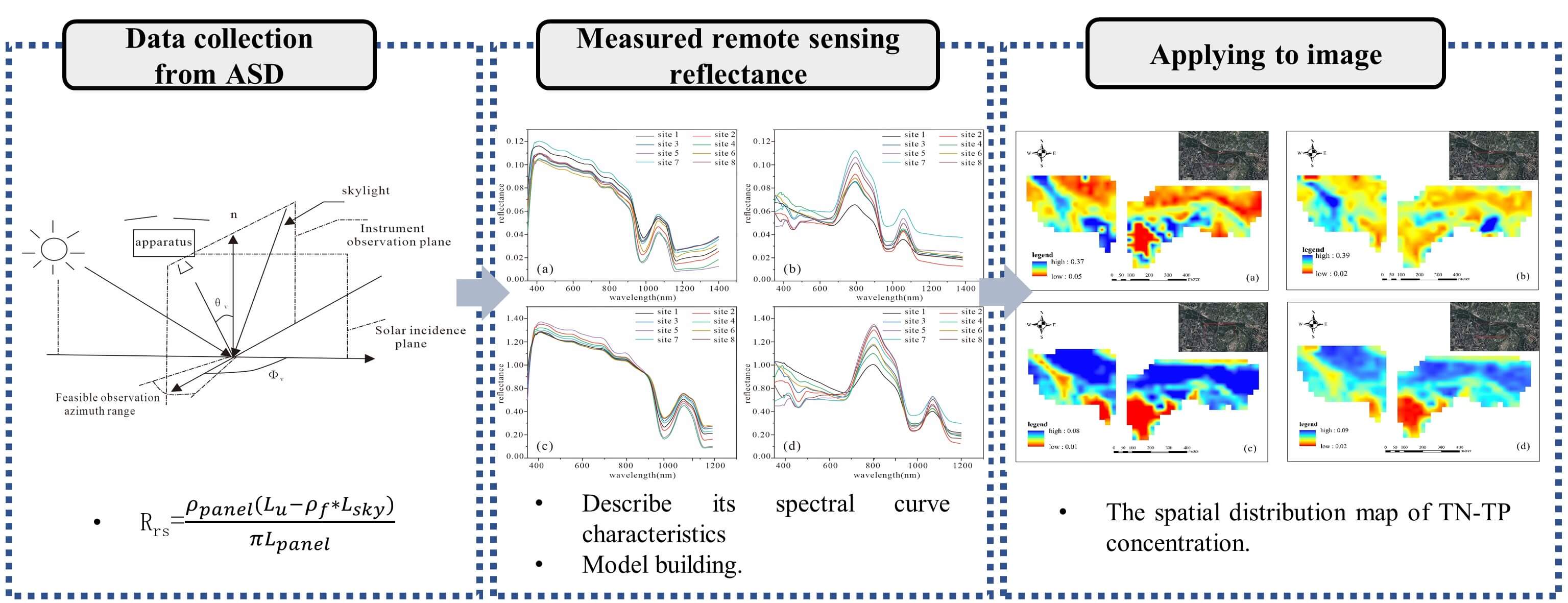
The Sha River, an important water system in Chengdu, China, was chosen as the research subject in this paper. The author collected water samples at various locations in the Sha River during January and June 2022 and analyzed the water’s spectrum using an ASD ground objective spectrometer. The collected water samples were sent to the laboratory to determine the concentrations of total nitrogen and total phosphorus. This study investigates the correlation between total total nitrogen, total phosphorus, and spectral data, with the intention of identifying the optimal band for quantitatively estimating total nitrogen and total nitrogen concentration. An estimation model is subsequently developed to establish a scientific foundation. The use of spectral sensors offers a novel approach for estimating water quality parameters on a large scale in the Sha River, Chengdu.
To validate the model’s applicability, Landsat9 remote sensing data was chosen for analysis. The Landsat9 satellite is considered superior to many other satellites because of its high spatial resolution and data availability. It offers a relatively comprehensive range of bands for water quality inversion, as indicated in Table 1. The Landsat9 image product (Image ID: LC09_L1TP_129039_20220421_20220421_02_T1), which is the closest to the field data collection date, was finally selected for case study.
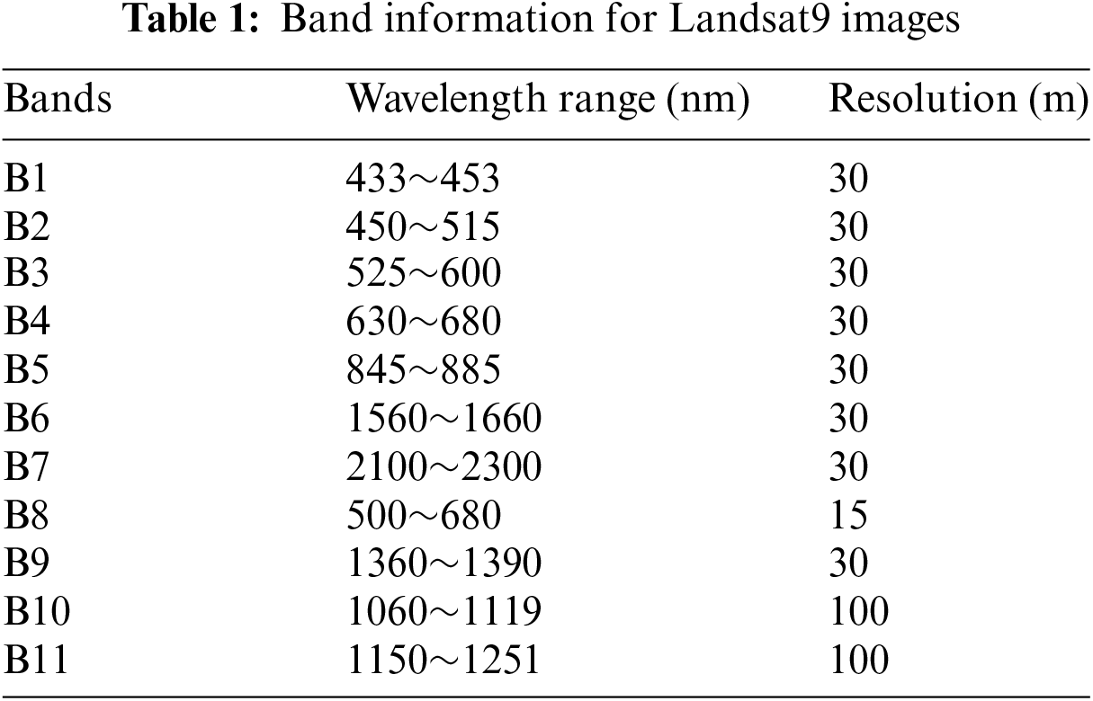
This Landsat data was downloaded from the United States Geological Survey (USGS, https://earthexplorer.usgs.gov/). ENVI5.3 is used to perform radiation and atmospheric correction on the image according to the image geometric observation method and time, combined with its spectral response function and field survey data. Then, according to the latitude and longitude, the corresponding Landsat9 image reflectance of the sampling point is extracted in ArcGIS10.8, and then the multi-temporal water body space-time information is extracted.
The Sha River is one of the three major urban rivers in Chengdu. It is part of the Minjiang River system (Fig. 1).
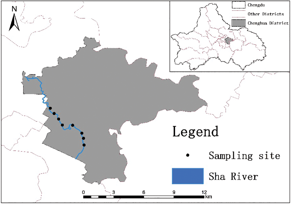
Figure 1: Location map of sampling points
The water samples used for this study were collected on January 05 and June 23, 2022. Fig. 1 illustrates the study area and the spatial distribution of the samples. Samples were collected at 15-minute intervals during the sampling process. The region’s complex anthropogenic conditions, along with various environmental factors such as wind speed and distance from the sampling location, contribute to a complex optical composition of surface water in the area. This composition results in a spectrum that is heavily influenced by suspended solids. A total of 1 L of water were collected at each site for subsequent laboratory analysis of TN and TP concentrations. After collection, the water samples were protected from light and stored in a refrigerator. The water temperature and pH of the water body were measured using a portable handheld analyzer, while the latitude, longitude, wind speed, and other environmental factors were recorded in the field. For example, Longitude, Latitude, Wind Velocity, etc., for further data processing.
Hyperspectral data were measured by Analytical Spectroscopy Device (ASD) FieldSpec4 produced by ASD Corporation (USA). The instrument parameters are as follows: the measurement spectrum range is 350–2500 nm, the wavelength accuracy is ±1 nm, the sampling time is 10 seconds/time, and the front field of view angle is 25°. For each measurement, the upward radiance (
Using the spectral data processing software ViewSpecPro to calculate the average value of the spectral curve of the sample. The spectral data is converted to ASCII format and then stored for further processing.
The determination of water quality parameters primarily involves direct measurements at the sampling site and subsequent physical and chemical analysis conducted in the laboratory. The field data collected for this study primarily includes measurements of water transparency as well as the latitude and longitude coordinates of the sampling points. The laboratory data primarily consists of the samples collected and sent to physical and chemical laboratories for analysis after being refrigerated. According to the specified indicators, the sampler should collect water samples from a depth of 50 cm below the water surface and distribute them equally into eight 500 ml brown glass bottles. At the same time, add H2SO4 to the brown bottles to keep the pH below 2. It was sent to the Sichuan Xiye Testing Laboratory for determination. The detection environment conditions were set at a temperature of 22°C and relative humidity of 55%. Determination of TN and TP followed the “Surface Water Environmental Quality Standard” (GB 11893-89), using alkaline potassium persulfate digestion ultraviolet spectrophotometry (GB 11894-89) and potassium persulfate digestion ammonium molybdate spectrophotometry (GB 11893-89) as the standard analysis methods.
Because of variations in measurement time and location, the spectrum exhibits variability. One approach to mitigate the impact of temporal and spatial variations on determining the absolute reflectance value is through the use of a spectrum normalization method. This method effectively reduces the influence of time and location differences on the determination of the absolute reflectance value. Normalized reflectance is calculated by dividing the reflectance at each wavelength by the average reflectance value across the entire wavelength range [26]. This study utilized the following formula for normalizing the albedo data of water bodies from remote sensing:
In the formula, the normalized water body remote sensing reflectance is the original calculated water body remote sensing reflectance, and n is the number of bands between 420 and 900 nm.
2.2.2 Spectral Differential Processing
Spectral differential technology allows for identifying shape changes in spectral data [27]. It rapidly determines spectral bending points and identifies the wavelength positions of maximum and minimum reflectivity. However, it has lower sensitivity to data amplitude. As a result, it finds wide applications in the field of remote sensing analysis.
First-order differential processing has the capability to remove linear or nearly linear backgrounds, mitigate the impact of noise spectrum on the target spectrum (which must be nonlinear), and minimize the influence of water on the reflection spectrum of water bodies [28]. Conversely, higher-order differential processing can effectively emphasize the weak points in the spectral signal caused by trace substances. First-order differential processing removes some of the linear and noise effects on the target spectrum. The calculation of the first-order differential in this study uses the following formula:
where
2.3 Model Verification and Evaluation
Half of the data are kept for this paper’s accuracy verification. Accuracy was assessed using the Root Mean Square Error (RMSE), Mean Absolute Percentage Error (MAPE), and Mean Absolute Error (MAE) [29]. The estimation error and model accuracy increase with value, and decrease with value.
In the formula,
3.1 Water Absorption-Reflection Characteristics in the Study Area
This paper aims to analyze the seasonal fluctuations of the spectral reflection curve of the water body in the Sha River by processing the spectral data curve using ENVI. Additionally, we describe the shape characteristics of the absorption bands in the spectrum. Fig. 2 illustrates the spectral reflectance curves of the Sha River captured during different seasons. The reflective spectral curves within the same season exhibit common features, while those from different seasons demonstrate notable differences. Consequently, the spectral data collected at various time periods within the same research area exhibit noticeable seasonal differences.
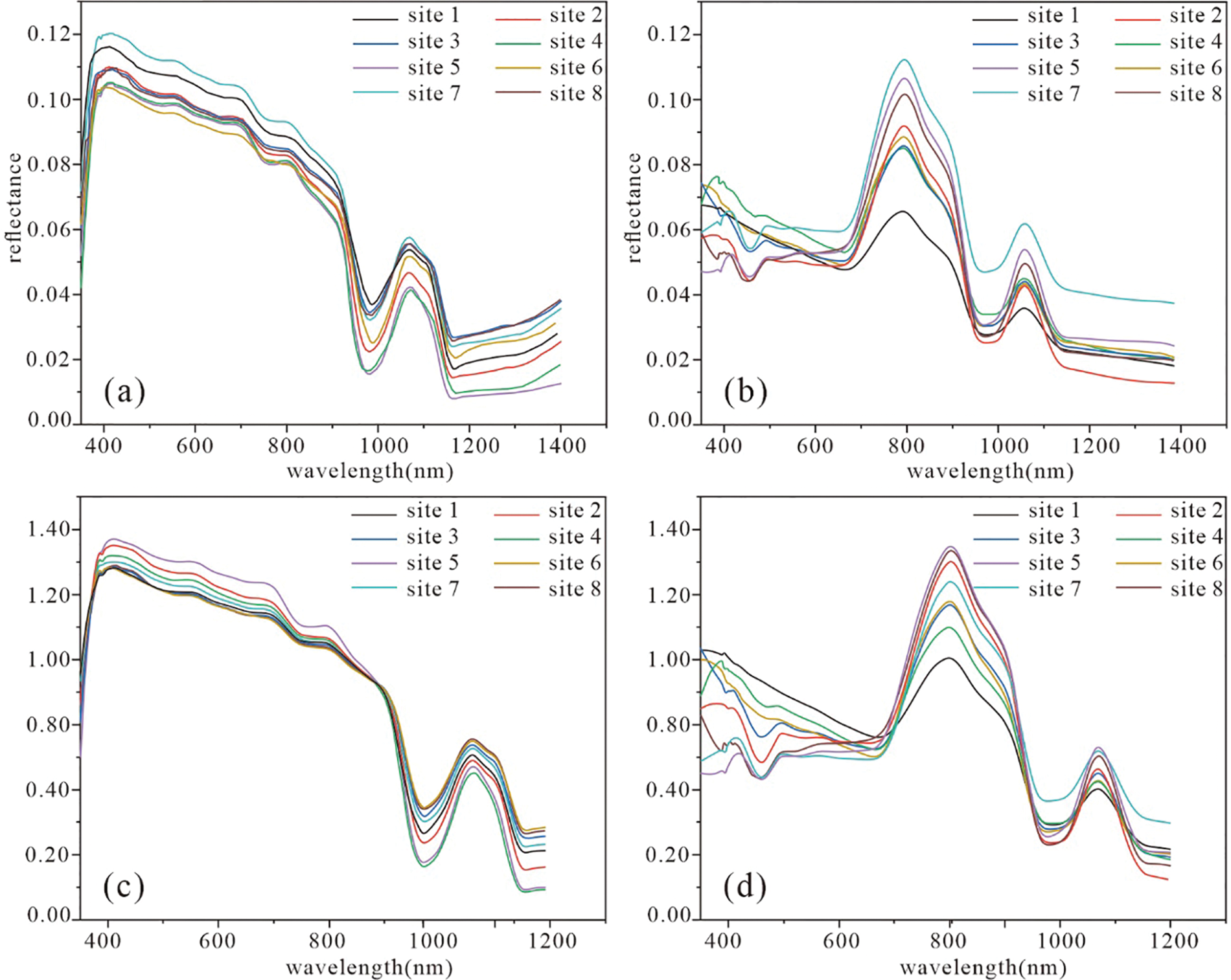
Figure 2: Raw spectral curves of January (a) and June (b) and normalized spectral curves of January (c) and June (d)
From Fig. 2, it can be seen that the spectral curves of water bodies vary significantly across different seasons. Overall, water bodies exhibit higher spectral reflectance during summer compared to winter. Therefore, normalizing the spectrum can mitigate the impact of temporal and spatial variations on the absolute reflectance value. The normalization results are depicted in Figs. 2c and 2d.
From a spectral perspective, the primary distinction between the winter and summer curves occurs at approximately 800 nm. During summer, a prominent reflection peak is observed at 800 nm, whereas the winter curve exhibits a more gradual change. The lower winter temperature hinders the formation of algae in water, leading to a decrease in chlorophyll and carotene concentration.
During summer, the reflectance of water in the 400–600 nm region of the spectral curve is reduced due to the light energy absorption by chlorophyll-a and yellow substances. Additionally, chlorophyll and carotene have a weak light energy absorption capability, further compounded by the scattering effect of cells. A prominent reflection peak is observed at 800 nm, serving as a quantitative benchmark for chlorophyll concentration. The absorption of phycocyanin in the 620–630 nm range induces a dip in the reflection spectrum. In addition, the strong absorption of chlorophyll-a around 670 nm results in additional valleys in the reflection spectrum [30]. The fluorescence peak in the 685–715 nm range is a crucial indicator of water containing algae, providing insight into the concentration of chlorophyll-a. It is worth noting that the position of the fluorescence peak exhibits a red shift phenomenon as the chlorophyll concentration increases. The reflectance in the range of 730–790 nm is relatively low due to the strong absorption of water in the near-infrared range. A small reflection peak around 760 nm may be attributed to the absorption of oxygen in the water. Another reflection peak is formed near 810 nm, possibly due to a combination of pure water properties and the scattering effect of suspended matter.
4.1 TN-TP Concentration Inversion Model
The objective of this study is to establish the relationship between the measured TN-TP concentration and the spectrum in order to analyze the seasonal impact on the water quality of the Sha River. The construction of the water quality inversion model typically involves analyzing the spectral characteristics of the water body to identify bands with strong responses. These bands are then used in correlation analysis with the concentration of the water quality parameter to establish the inversion model based on the principle of the largest correlation coefficient. This study examines the correlation between TN-TP, normalized remote sensing reflectance data, and multi-order differential algorithm spectrum in different seasons using Pearson correlation analysis [31]. The parameter with the highest correlation coefficient is then selected for water quality parameter inversion. Pearson correlation analysis is a statistical method used to assess the strength of correlation between two or more random variables. The correlation coefficient’s magnitude indicates the extent of closeness between variables, and is represented by formula (7):
Correlation analysis was conducted between the TN-TP concentration and the normalized reflectance data of each point. The maximum positive and negative correlation coefficients in January and June were obtained through correlation analysis (Figs. 3b, 3c). The findings indicate that the correlation between the multi-order differential data and TN-TP was significantly higher compared to that of the normalized reflectance data. Therefore, the multi-order differential approach demonstrates a robust advantage in establishing the TN-TP model.
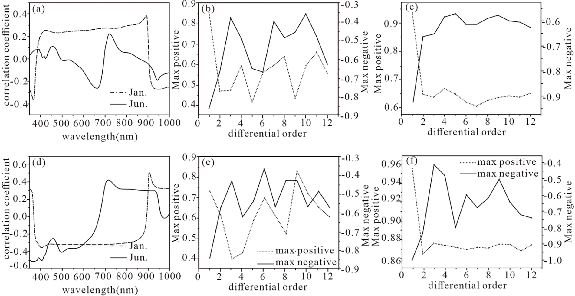
Figure 3: TN-TP spectral correlation coefficients (a) the correlation coefficient between normalized data and TN; (b) the maximum positive and negative correlation coefficient between different differential orders and TN concentration in January; (c) the maximum positive and negative correlation coefficient between different differential orders and TN concentration in June; (d) the correlation coefficient between normalized data and TP; (e) the maximum positive and negative correlation coefficient between different differential orders and TP concentration in January; (f) the maximum positive and negative correlation coefficient between different differential orders and TP concentration in June negative correlation coefficient
Based on the correlation analysis conducted above, the differential single-band with a relatively high correlation was chosen as the inversion factor for TN-TP. The fitting was performed using SPSS software with the quadratic polynomial, exponential, power function, and linear function. After evaluating the fitting effect of the TN model using data collected in January, it was determined that the power function at 586 nm exhibited the highest performance, with R2 = 0.95 and F = 164.57. In contrast, during June, the exponential model at 477 nm yielded the most satisfactory fitting effect, with a fitting coefficient R2 = 0.93 and F = 80.95 at a significance level of p < 0.01.
During the fitting model in January, the differential value of 851 nm with a 1 nm interval demonstrated the best fitting effect for TP, with an R2 value of 0.78. However, the fitting effect in June surpassed that of January, reaching an R2 value of 0.96 for TP.
4.1.3 Model Evaluation and Testing
Utilize the remaining four sample points to test, the RMSE, MAPE, and MAE were calculated (Table 2), considering factors such as the R2 and F values of the regression model and RMSE, MAPE, MAE between the predicted and measured values, the best model is determined. Fig. 4 is the scatter diagram of the predicted value and the measured value of the model and the root mean square error of the predicted value. It can be seen from Fig. 4 that it is used for verification The relative error of the sample points is within 20%, indicating that the model has good prediction results and stability.
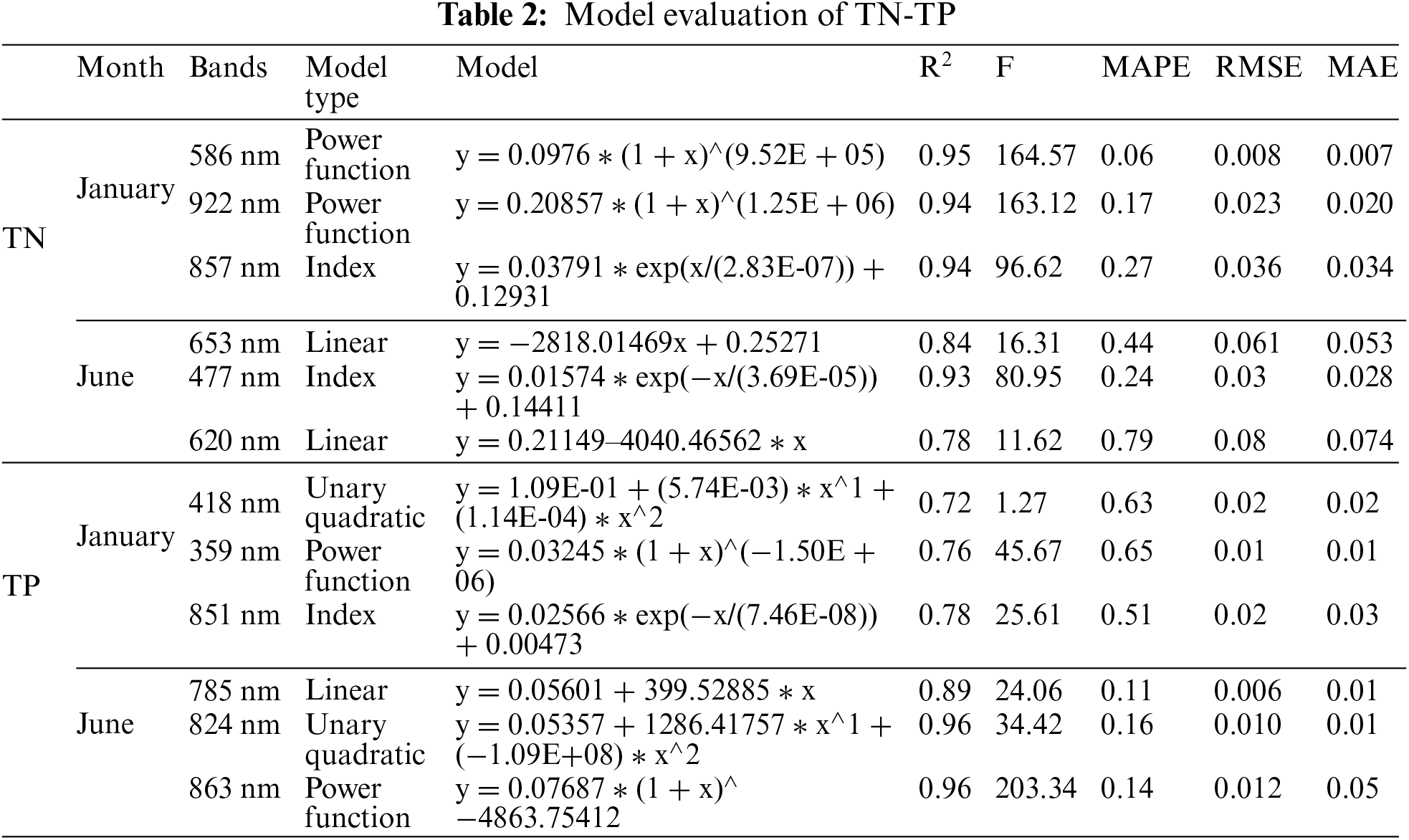
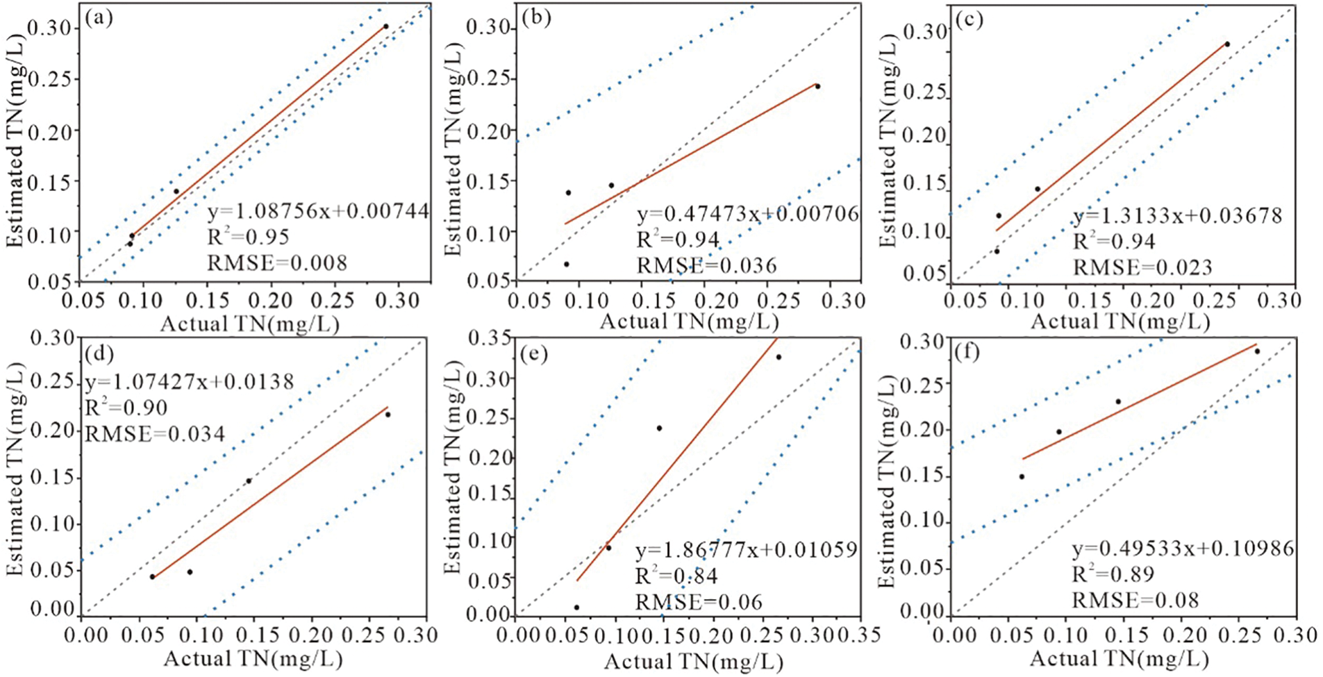
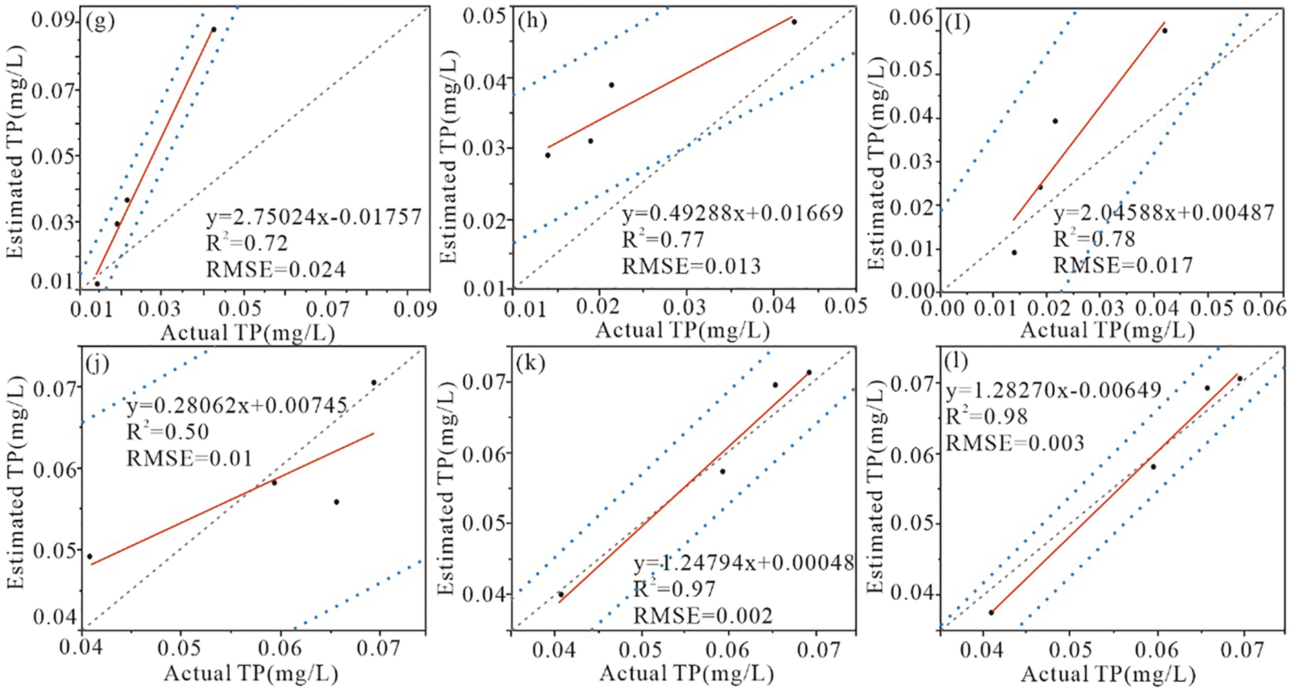
Figure 4: Comparison of predicted and measured values of TN-TP concentration. (a) January 586 nm, (b) January 857 nm, (c) January 922 nm, (d) June 620 nm, (e) June 653 nm, (f) June 477 nm, (g) January 418 nm, (h) January 359 nm, (i) January 851 nm, (j) June 824 nm, (k) June 863 nm, (l) June 785 nm. The solid red line represents the regression line between predicted and observed values. The double blue dashed line is the 95% prediction band and the gray dashed line is the y=x line
4.2 TN-TP Concentration Inversion Model
The best models are applied to Landsat9 remote sensing satellite images, and the Spatial Model module in ArcMAP was used to build a spatial model of TN-TP inversion, and the spatial distribution of TN-TP concentration in part of the Sha River basin was obtained after image by image calculation (Fig. 5).
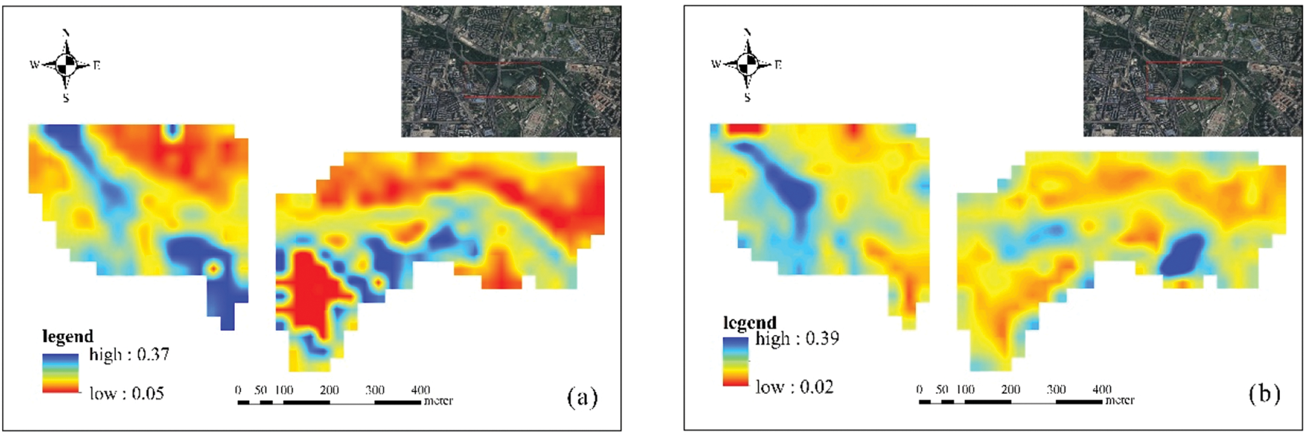
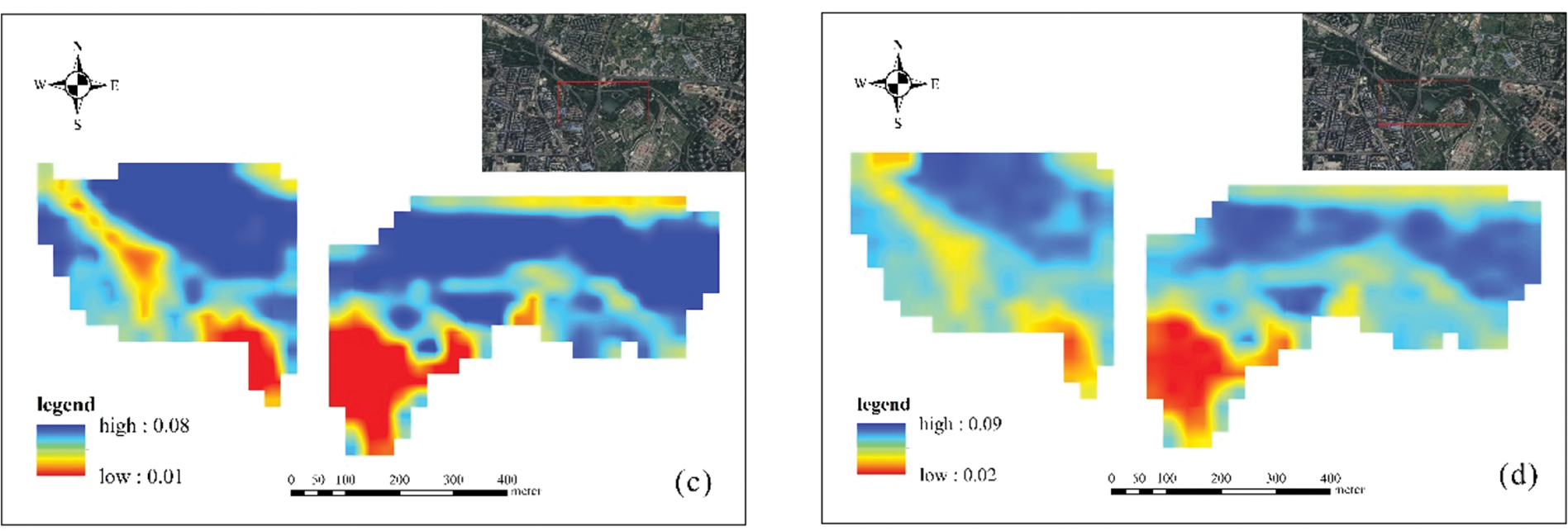
Figure 5: The spatial distribution map of TN-TP concentration. (a) Spatial distribution of TN concentration in January; (b) Spatial distribution of TN concentration in June; (c) Spatial distribution of TP concentration in January; (d) Spatial distribution of TP concentration in June
The best model was used to invert the spatial distribution of TN and TP by combining 2/3 of the measured data with the reflectance data of Landsat images, in order to verify the model results. Fig. 5 demonstrates the accuracy of the inversion model in the application of Landsat image data. The distribution of TN and TP concentrations obtained by the inversion model closely resemble the measured concentration distribution when applied to the image. The TN concentration varies across different months. This difference is primarily due to temperature effects on algae growth, resulting in changes in TN concentration in the water body, while the variation in TP concentration remains small across different months. The concentrations of TN and TP were higher in the middle of the water body from a spatial perspective. Additionally, they exhibit better discrimination and provide richer distribution details in different concentration regions.
At present, the inversion mechanism of total nitrogen and total phosphorus based on hyperspectral data remains unclear, hence the reliance on empirical models for inversion. The inversion effect of total phosphorus is superior to that of total nitrogen. This is primarily due to the susceptibility of the 530 nm nitrogen-sensitive band to interference from non-pigmented substances and xanthin in water, and the influence of pure water signals on the 693 nm band. In contrast, the sensitive band of total phosphorus is relatively less affected compared to total nitrogen. Moreover, Researchers have observed covariation during their study [32]. The following conclusions were drawn from this investigation:
(1) The Sha River in Chengdu is very different. Winter is the dry season of the Sha River, with little precipitation, small river runoff, and shallow river water; the water level of the Sha River rises in summer and the precipitation increases. In terms of total nitrogen and total phosphorus content, the difference between the two is not obvious, but the corresponding spectral curve difference is more obvious. The difference between the two is most obvious at 800 nm, and after correlation analysis it was concluded that the inversion model based on this range is better.
(2) The differential method is highly sensitive to the concentration of total nitrogen and total phosphorus, enabling effective extraction of weak signals. The inversion model, generated using the differential method and multiple linear regression, exhibits relatively high prediction accuracy. For the total nitrogen model, the power function model at 586 nm demonstrates the best fitting effect, with a fitting coefficient of R2 = 0.95 and F = 164.57 at a significance level of p < 0.01. The exponential model at 477 nm in June demonstrates the best fitting effect with a fitting coefficient of R2 = 0.93 and F = 80.95 at the significance level of p < 0.01. For the total phosphorus model, the differential value at 851 nm in January results in the best fitting effect with the exponential model, showing an R2 value of 0.78 and F = 20.61 at the significance level of p < 0.01. Moreover, the fitting effect in June outperforms that of January, wherein the differential values at 824 and 863 nm contribute positively. The one-dimensional quadratic model and the linear model used for fitting total phosphorus achieved R2 values of 0.96, with respective F-values of 34.42 and 203.34. Furthermore, the relative error between the predicted and sample points was within 20%, indicating the model’s excellent prediction accuracy and stability.
The hyperspectral inversion of total nitrogen and total phosphorus is still in the exploratory stage and requires further investigation into molecular spectroscopy and optical mechanisms to improve the inversion model. This research is in its early stages, and the current collection of experimental data is insufficient. In the future, the scope of study will be expanded both temporally and spatially, and the data set will be enlarged for more comprehensive exploration.
Acknowledgement: We are very grateful to the USGS EarthExplore for providing the Landsat9. In addition, we thank the anonymous reviewers whose comments improved the manu-script.
Funding Statement: This study is funded by the Gansu Provincial Science and Technology Plan Project, Innovation Base and Talent Project (Project Number: 21JR1RA284).
Author Contributions: The authors confirm contribution to the paper as follows: study conception and design: Na Guo; data collection: Yaping Luo, Xinchen Wang, and Jie Wu; analysis and interpretation of results: Yaping Luo, Na Guo; draft manuscript preparation: Shuming Peng, Liu Dong. All authors reviewed the results and approved the final version of the manuscript.
Availability of Data and Materials: This Landsat data was downloaded from the United States Geological Survey (USGS, https://earthexplorer.usgs.gov/).
Conflicts of Interest: The authors declare that they have no conflicts of interest to report regarding the present study.
References
1. Mihiranga, H. K. M., Jiang, Y., Sathsarani, M. G. S., Li, X., Ritigala, T. et al. (2022). Identification of rainy season nitrogen export controls in a semi-arid mountainous watershed, North China. Science of the Total Environment, 839, 156293. [Google Scholar] [PubMed]
2. Schindler, D. W. (1977). Evolution of phosphorus limitation in lakes. Science, 195, 260–262. [Google Scholar] [PubMed]
3. Chen, Z. X., Yu, L., Liu, W. G., Lam, M. H. W., Liu, G. J. et al. (2013). Nitrogen and oxygen isotopic compositions of water-soluble nitrate in Taihu Lake water system, China: Implication for nitrate sources and biogeochemical process. Environmental Earth Sciences, 71, 217–223. [Google Scholar]
4. Duan, W., Takara, K., He, B., Luo, P., Nover, D. et al. (2013). Spatial and temporal trends in estimates of nutrient and suspended sediment loads in the Ishikari River, Japan, 1985 to 2010. Science of the Total Environment, 461–462, 499–508. [Google Scholar] [PubMed]
5. Wang, J., Fu, Z., Qiao, H., Liu, F. (2019). Assessment of eutrophication and water quality in the estuarine area of Lake Wuli, Lake Taihu. China Science of the Total Environment, 650, 1392–1402. [Google Scholar] [PubMed]
6. Tang, C., Li, Y., Acharya, K. (2016). Modeling the effects of external nutrient reductions on algal blooms in hyper-eutrophic Lake Taihu, China. Ecological Engineering, 94, 164–173. [Google Scholar]
7. Paerl, H. W., Xu, H., McCarthy, M. J., Zhu, G., Qin, B. et al. (2011). Controlling harmful cyanobacterial blooms in a hyper-eutrophic lake (Lake Taihu, ChinaThe need for a dual nutrient (N & P) management strategy. Water Research, 45, 1973–1983. [Google Scholar] [PubMed]
8. Carlson, R. E. (1977). A trophic state index for lakes. Limnology and Oceanography, 22, 361–369. [Google Scholar]
9. Al-Fahdawi, A. A., Rabee, A. M., Al-Hirmizy, S. M. (2015). Water quality monitoring of Al-Habbaniyah Lake using remote sensing and in situ measurements. Environmental Monitoring and Assessment, 187, 367. [Google Scholar] [PubMed]
10. Palmer, S. C. J., Kutser, T., Hunter, P. D. (2015). Remote sensing of inland waters: Challenges, progress and future directions. Remote Sensing of Environment, 157, 1–8. [Google Scholar]
11. Arabi, B., Salama, M., Wernand, M., Verhoef, W. (2016). MOD2SEA: A coupled atmosphere-hydro-optical model for the retrieval of chlorophyll-a from remote sensing observations in complex turbid waters. Remote Sensing, 8, 722. [Google Scholar]
12. Jiang, L., Li, Y., Zhao, X., Tillotson, M. R., Wang, W. et al. (2018). Parameter uncertainty and sensitivity analysis of water quality model in Lake Taihu, China. Ecological Modelling, 375, 1–12. [Google Scholar]
13. Dev, P. J., Sukenik, A., Mishra, D. R., Ostrovsky, I. (2022). Cyanobacterial pigment concentrations in inland waters: Novel semi-analytical algorithms for multi- and hyperspectral remote sensing data. Science of the Total Environment, 805, 150423. [Google Scholar] [PubMed]
14. Song, Z., Chomicki, K. M., Drouillard, K., Weidman, R. P. (2023). Effects of detection limits on spatial modeling of water quality in lakes. Science of the Total Environment, 864, 161052. [Google Scholar] [PubMed]
15. Niroumand-Jadidi, M., Bovolo, F., Bruzzone, L. (2019). Novel spectra-derived features for empirical retrieval of water quality parameters: Demonstrations for OLI, MSI, and OLCI. IEEE Transactions on Geoscience and Remote Sensing, 57, 10285–10300. [Google Scholar]
16. Tehrani, N. A., Janalipour, M., Babaei, H. (2021). Estimating water surface chlorophyll-a concentration by big remote sensing data in the persian gulf. Bushehr Remote Sensing in Earth Systems Sciences, 4, 87–95. [Google Scholar]
17. Wei, J., Wang, M., Mikelsons, K., Jiang, L., Kratzer, S. et al. (2022). Global satellite water classification data products over oceanic, coastal, and inland waters. Remote Sensing of Environment, 282, 113233. [Google Scholar]
18. Luo, D., Xu, B., Li, Z. M., Sun, H. (2020). Biogeographical divides delineated by the three-step landforms of China and the East China Sea: Insights from the phylogeography of Kerria japonica. Journal of Biogeography, 48, 372–385. [Google Scholar]
19. Liu, S., Glamore, W., Tamburic, B., Morrow, A., Johnson, F. (2022). Remote sensing to detect harmful algal blooms in inland waterbodies. Science of the Total Environment, 851, 158096. [Google Scholar] [PubMed]
20. Gao, Z., Shen, Q., Wang, X., Peng, H., Yao, Y. et al. (2021). Spatiotemporal distribution of total suspended matter concentration in Changdang Lake based on in situ hyperspectral data and sentinel-2 images. Remote Sensing, 13, 4230. [Google Scholar]
21. Gerhards, M., Schlerf, M., Mallick, K., Udelhoven, T. (2019). Challenges and future perspectives of multi-/hyperspectral thermal infrared remote sensing for crop water-stress detection: A review. Remote Sensing, 11, 1240. [Google Scholar]
22. Wang, Z., Sakuno, Y., Koike, K., Ohara, S. (2018). Evaluation of chlorophyll -a estimation approaches using iterative stepwise elimination partial least squares (ISE-PLS) regression and several traditional algorithms from field hyperspectral measurements in the Seto Inland Sea, Japan. Sensors, 18, 2656. [Google Scholar] [PubMed]
23. Pahlevan, N., Smith, B., Schalles, J., Binding, C., Cao, Z. et al. (2020). Seamless retrievals of chlorophyll-a from Sentinel-2 (MSI) and Sentinel-3 (OLCI) in inland and coastal waters: A machine-learning approach. Remote Sensing of Environment, 240, 111604. [Google Scholar]
24. Fargette, M., Raouani, N. (2022). La genèse systémique d'empreinte pour une maîtrise de l'observation de la Terre. Revue Internationale de Géomatique, 31(1), 135–197. [Google Scholar]
25. Kutser, T., Hedley, J., Giardino, C., Roelfsema, C., Brando, V. E. (2020). Remote sensing of shallow waters–A 50 year retrospective and future directions. Remote Sensing of Environment, 240, 111619. [Google Scholar]
26. Kumar Jally, S., Kumar Mishra, A., Balabantaray, S. (2019). Estimation of Trophic State index of Chilika Lake using Landsat-8 OLI and LISS-III satellite data. Geocarto International, 35, 759–780. [Google Scholar]
27. Li, S., Chen, F., Song, K., Liu, G., Tao, H. et al. (2022). Mapping the trophic state index of eastern lakes in China using an empirical model and Sentinel-2 imagery data. Journal of Hydrology, 608, 127613. [Google Scholar]
28. Kallio, K., Kutser, T., Hannonen, T., Koponen, S., Pulliainen, J. et al. (2001). Retrieval of water quality from airborne imaging spectrometry of various lake types in different seasons. Science of the Total Environment, 268, 59–77. [Google Scholar] [PubMed]
29. Matthews, M. W. (2011). A current review of empirical procedures of remote sensing in inland and near-coastal transitional waters. International Journal of Remote Sensing, 32, 6855–6899. [Google Scholar]
30. Yacobi, Y. Z., Gitelson, A., Mayo, M. (1995). Remote sensing of chlorophyll in Lake Kinneret using highspectral-resolution radiometer and Landsat TM: Spectral features of reflectance and algorithm development. Journal of Plankton Research, 17, 2155–2173. [Google Scholar]
31. Nechad, B., Ruddick, K. G., Park, Y. (2010). Calibration and validation of a generic multisensor algorithm for mapping of total suspended matter in turbid waters. Remote Sensing of Environment, 114, 854–866. [Google Scholar]
32. Neill, M. (2005). A method to determine which nutrient is limiting for plant growth in estuarine waters–at any salinity. Marine Pollution Bulletin, 50, 945–955. [Google Scholar] [PubMed]
Cite This Article
 Copyright © 2023 The Author(s). Published by Tech Science Press.
This work is licensed under a Creative Commons Attribution 4.0 International License , which permits unrestricted use, distribution, and reproduction in any medium, provided the original work is properly cited.
 Downloads
 Citation Tools