Integration of Frequency Ratio-Analytical Hierarchical Process (FR-AHP) in GIS for Measuring Campus Spatial Accessibility Index

1  Introduction

Walking and cycling are known as active transport that use physical movement involving walking on foot and non-motorized vehicles. Active transport can be categorized as sustainable transport because it can decrease noise from motorized vehicles and air pollution. It offered individual and community health and well-being [1,2]. These days, active transports are used to enhance the accessibility of public transportation services. The journey to access public transportation is known as the First and Last Mile (FLM), where active transport is one of the mediums. It is important to ensure the public transport is accessible by using active transport. Hence, one of the key concepts for measuring this is spatial accessibility.

Spatial accessibility for active and public transportation is an analysis using a GIS-based model in order to determine the accessibility of transportation in the study area. The method to measure Spatial Accessibility depends on the factors used. Spatial accessibility can be used in transportation planning to analyze the relationship between transportation and physical factors, and also to study the impact of transportation policies [3].

There are several methods that have been applied widely in measuring spatial accessibility, with each having advantages and limitations. The first technique is the Two-Step Floating Catchment Area (2SFCA), which is known for its capacity to incorporate the supply and demand in measuring accessibility. However, it is highly sensitive to the selection of catchment thresholds and neglects other important criteria in measuring accessibility, such as socio-economic. Analytical Hierarchical Process (AHP), on the other hand, is one of the most popular Multicriteria Decision Analysis MCDA methods as it provides a systematic framework for measuring accessibility based on human preferences on multiple criteria. However, it has limitations due to potential inconsistencies in the decision-making process. The third technique, Frequency-Ratio (FR), is a data-driven method that objectively quantifies the relationships between influencing factors and accessibility; however, it does not incorporate human preferences in the process.

Due to these methodological gaps, the ensemble method of FR-AHP has been proposed, which is capable of integrating the empirical rigor of FR with the structured multicriteria framework of AHP, thereby producing a more comprehensive and reliable measure of spatial accessibility. In this study, spatial accessibility was measured by using the MCDA concept with GIS-based FR and AHP methods. FR were used to calculate the estimation index values between physical factors and the study area, combined with AHP to analyze the accessibility and produce an accessibility model. With these two methods, the accessible area of active transportation and public transport was found.

Thus, this study was conducted aiming to measure the Campus Spatial Accessibility Index (CSAI) for active mobility and public transportation around a public university in Shah Alam (Fig. 1). The factors and the impact of physical factors were used to analyze the accessibility and were used to create the CSAI map. From the CSAI map, the accessibility map of active mobility and public transportation around the campus has been produced, referring to the suitable location with access to active and public transportation accessibility. The CSAI maps could help students become more familiar with accessing the campus.

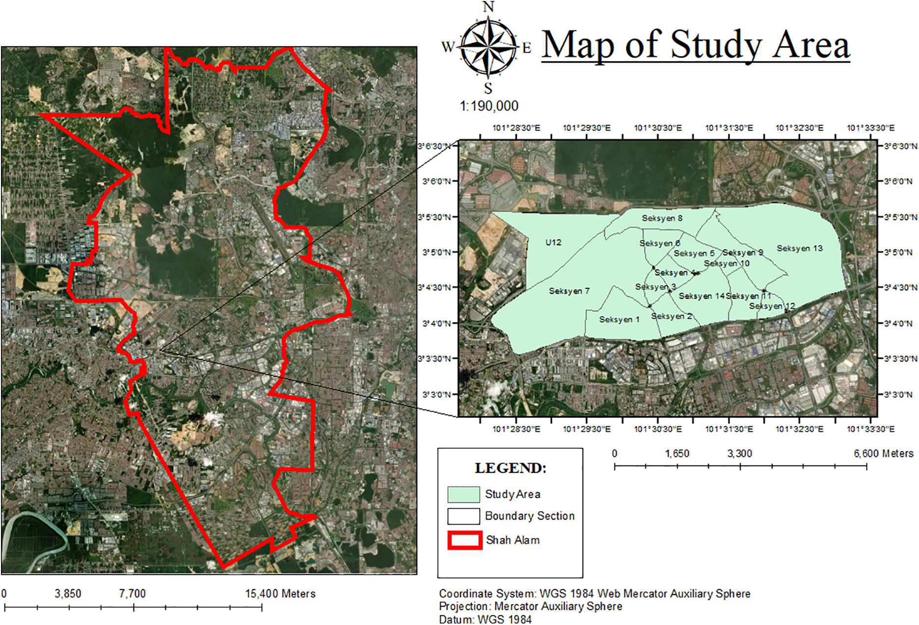
Figure 1: Study area

2  Literature Review

2.1 Spatial Accessibility

Active transportation is non-motorized and fully relies on human power for travel. Some examples of active transportation are walking, skateboarding, and cycling. Walking is a physical movement that involves movement by foot, and cycling is a movement using non-motorized vehicles such as bicycles. Therefore, active transportation is a movement that offers many benefits in terms of health and a sustainable transport network. Walking is an ideal activity for people as it is a safe, accessible, and cost-free activity [4]. For example, some people preferred to walk and cycle to the nearest areas, such as school, the shop lot, and also walk inside the shopping mall. It also helps in improving the air quality and improving vibrancy and livability since there are no vehicles used on roads.

Spatial accessibility for active transportation can be referred to as a distinctive measurement that connects two locations and the spatial distribution of physical movement with the networks of transport systems. Nowadays, the increasing population in Malaysia results in an increasing number of vehicles on the road. However, traffic congestion makes people choose active transport as their main transportation to reach the destination [5,6]. Unfortunately, there is a weakness in terms of the accessibility of active transportation. The accessibility of active transportation could be affected by several factors, such as construction and road network, which leave people with no other choice but to use motorized vehicles to move [7]. Therefore, people in the area may find it difficult to use active transportation as their main mode of transportation due to the lack of accessibility. Promoting active transportation requires a high understanding of accessibility indicators, which is useful for planning and evaluating accessibility [8].

Public transportation is an important element of a public transportation system that allows mobility without the need to use any private vehicle, such as a car or motorcycle, especially when the distance is too great for active mobility [9]. Public transportation also includes active transportation, where people need to walk or cycle to reach the public transportation station or transit stop [10]. For example, people with limited accessibility to public transportation need to walk or cycle to the end location of public transportation stations, such as bus terminals, commuter stations, and bus stops. This is due to the different service coverage, irregular service frequencies, limited infrastructure supporting the first-last mile, as well as connectivity issues between the services in several demand areas, which then lead to inequitable access [11].

Access to public transport should be improved to facilitate the movement of people to public transport stations closer to their residential areas [12]. Usually, most public transport stations are close to urban areas, and the residents in this area can access public transport stations easily. However, with the use of spatial accessibility measurement, it is possible to find areas with low accessibility, so that they can be further improved to enhance the FLM and promote a seamless travel experience when using public transportation. Hence, with spatial accessibility, car-reliance may be reduced as more people will use public transport to travel, resulting in a more sustainable city and lifestyle, which is the global goal these days.

Facilities and amenities should be accessible by active transportation to enhance walkability [13]. It includes access network from the demand point to the destination. University campus is one of the education facilities in urban area. Hence, campus spatial accessibility could be used to measure the accessibility from the campus into the nearest area around the campus. In campus spatial accessibility, the demand point could be the areas around the campus. The accessibility analysis aims to find out and analyze the access from the area near the campus to the campus [14]. The determination of campus spatial accessibility for active transportation can help students choose walking or cycling as their transportation to the campus, as walking and cycling activities can be beneficial to health, such as reducing body weight and promoting a healthy lifestyle [15,16].

There are four (4) factors to determine the quality of public transportation services, which include accessibility, availability, affordability, and acceptability [17]. Spatial accessibility allows students to make a choice whether to use a public transportation service, such as a public bus, or use other public transportation to reach the destination. The spatial accessibility is important as planning, preparation, and waiting time are needed to access a facility [18]. Campus spatial accessibility could also provide access for students to reach nearby locations such as the shop lots near campus areas. Therefore, campus spatial accessibility is beneficial for students to move around the nearby campus areas by using alternative active transportation routes or public transportation routes that have been defined using spatial accessibility.

The aim of this measurement is to identify areas with low accessibility so that they can be improved. There are many factors influencing the accessibility, including physical factors. The determination of physical factors that affect travel behavior is a key in modelling transport accessibility [19]. From previous studies, there are various factors listed as factors that can be used to find the area of accessibility. The factors used to measure transport accessibility for university students include population density, intersection density, building density, public transport service area, land use, slope, and elevation. All the factors were selected based on the structure near the study area. The selection factor of population density is to measure the number of households and the number of students in the area. Meanwhile, intersection density was chosen to measure the walkability of connecting streets. The factor of building density can be used to study the location areas, such as residential areas, shop lot areas, and also to determine active transport movement. In order to determine the accessibility of public transportation, the public transport service area is used to measure the accessibility from the demand area. Public transport accessibility will be evaluated by estimating the distance from the nearest public station to the demand area, such as the campus area. The factors of land use, slope, and elevation a natural environment that is used in determining a surface that is easy to use as an accessibility area. With a combination of these factors, the accessibility index can be known and determined.

There are also other factors that are used as factor influence the accessibility. The factors used to measure accessibility are the frequency of proximity stops, time, cost, destination, user’s need, and choice of transport [19,20]. The selection of proximity stops and the trip frequency factor is used to determine the frequency of public transport stops at an access point. This factor is the common accessibility elements to analyze the situation and is used for planning and verifying the efficiency of measures [19,20]. Next, the influencing factor of the destination will affect the cost rate of accessibility. The destination chosen by people will determine the possibility and estimated time required to reach the destination, and also the cost that will be incurred throughout the journey. Other than that, the choices of transport mode will also give a prediction for travel speed and duration. Considering all the factors above, the analysis of accessibility can be conducted.

2.2 GIS in Measuring Spatial Accessibility

Measuring campus spatial accessibility relies on two (2) main concepts, which are location and distance between origin and destination. In addition, it is also important to consider the type of spatial accessibility, such as topological accessibility to measure nodes and paths, and second, the contiguous accessibility to measure accessibility over a surface. Therefore, the concept and category of spatial accessibility are important elements in determining the technique that will be used to measure the spatial accessibility. Next, connectivity and total accessibility are the basic elements that need to be involved in measuring accessibility.

There are various techniques that could be used to measure campus spatial accessibility by using a GIS-based model. There are several things that need to be considered in choosing a suitable technique, such as the type of accessibility that needs to be measured, the connectivity of accessibility, the equation used to measure the accessibility, and the geographic and potential accessibility [21]. In defining accessibility, the impact of infrastructure and transport development needs to be considered because accessibility is linked with economic and social opportunities [22]. The ability of a location to be reached from various locations is measured by its accessibility. Therefore, a significant factor in determining accessibility is the capacity and configuration of the transportation infrastructure.

To measure accessibility, the shortest paths between two different locations need to be calculated. The shortest paths of accessibility can be calculated with the minimum number of paths, and the accessibility measurement is known as the Shimbel accessibility matrix (D-matrix). This matrix provides the minimum distance between each node of the network for measuring spatial accessibility. Spatial accessibility considers that the accessibility of a location is a summation of all distances between different locations.

2.2.1 Two-Step Floating Catchment Area (2SFCA)

The Two-Step Floating Catchment Area (2SFCA) is a commonly used method to measure spatial accessibility [23]. It has been used in a number of recent studies in measuring spatial accessibility [23–26]. This method was used to define the catchment areas within a specific distance from demand points. The measurement of spatial accessibility by using 2SFCA methods for multiple transportation modes will provide more realistic accessibility compared to single-mode methods. In measuring spatial accessibility, 2SFCA is one of the methods to advance the quality of spatial accessibility measurement.

In the 2SFCA method, the catchment area is defined as the demand area of accessibility into destination areas. With various improvements of 2SFCA methods, such as improvements in distance-decay functions, variable catchment area, the effect among demanders or facilities, and the improvements of multiple types of transportation, this method is more powerful and strengthens the capability of the 2SFCA method for different types of data. Based on previous studies, the advancement of the 2SFCA method was measured by two steps: first, the supply-to-demand ratios for each facility were searched within the catchment areas, and second, the sum of all supply-to-demand ratios of all facilities that are located in the catchment area.

2SFCA could aid in the evaluation of accessibility by considering both the supply and demand represented by the population within a catchment area. Although the method is straightforward, its effectiveness is highly dependent on the threshold chosen for the measurement. In addition, the method tends to oversimplify accessibility by only focusing on the spatial proximity while disregarding the other factors that may influence accessibility, including socio-economic and behavioral factors.

2.2.2 Frequency Ratio (FR)

There are various methods in Bivariate Statistical Analysis (BSA) such as Weight of Evidence (WoE), Evidential Belief Functions (EBFs), and Frequency Ratio (FR). FR is one of the simple bivariate statistical methods to implement with accurate results [27]. FR was used to determine the relationship between two variables, such as the main studies and the conditioning factors. The bivariate statistical model expresses the possibility of two variables occurring [19]. For example, FR analysis can be used to determine the relationship between campus spatial accessibility and the physical factors. FR is a famous bivariate statistical model and is frequently used to measure and explain the occurrence of various natural hazards in various fields.

FR is also known as the weightage of parameter values from the frequency ratio model and an equation created using the logistic regression model to create the susceptibility map [28]. FR can be measured using various types of equations according to the data that needs to be calculated. Analytical Hierarchical Process (AHP).

AHP is an MCDA weighing method that can be used to determine the main alternative decisions by comparing the decision of physical factors. AHP can also be defined as an MCDA technique that can be used to determine the priorities of alternative decisions by comparing the decision criteria. The AHP is the most comprehensive method of MCDA [29,30].

AHP can be used based on three (3) principles, such as decomposition, comparative judgment, and synthesis of priorities [29,30]. In the decomposition principle, a decision problem needs to be decomposed into a hierarchy to capture the essential elements of the problem. For the comparative judgment principle, an assessment of pairwise comparisons of the elements within the given level of the hierarchical structure according to the main of the next-higher level. The pairwise comparison method uses a scale between 1 and 9 to rate the preferences with respect to a pair of criteria [29]. The principle of synthesis aims to combine each of the derived ratio-scale and priorities into the various levels of hierarchy, and it also constructs a composite set of priorities for the elements at the lowest level of the hierarchy. For spatial accessibility measurement, AHP was used to determine the relative significance of different physical factors in combination with the FR method, which will be further discussed in the next section [19].

2.2.3 FR-AHP

The combination of FR-AHP is an ensemble modeling technique. The FR-AHP is a joining technique that joins two different models into one model to develop predictive capability [31–34]. The weightage of each parameter was calculated using one model, AHP, through the pairwise comparison method. The AHP method is used to assign the most important weights to each parameter after normalizing the Eigenvector (EV) values from inconsistent pairwise comparison matrices. In comparison, the FR model can be defined as the proportion of parameters for each input layer as the ratio of each pixel in a category of a class of factor [32].

Given the limitations of other methods as discussed in this section, there is a clear need for an approach that balances both objectivity and subjectivity in the measurement of spatial accessibility. The FR-AHP method provides this integration by combining the statistical robustness of FR with the structured expert-driven framework of AHP. FR objectively identifies the relative importance of factors based on observed data, while AHP allows expert input to refine and adjust weights according to local priorities and contextual realities. This complementary framework mitigates the subjectivity of AHP and the rigidity of FR, resulting in more reliable and policy-relevant measures of accessibility.

3  Methodology

Fig. 2 shows the workflow of the methodology used in deriving the CSAI. After the factors had been determined, the data collection started to derive Trip Location Data, which was then used to develop the FR model, and then, combined with AHP to measure the weightage for each of the factors. Then, the weightage was used as parameters in deriving an index model for the CSAI by using Weighted Overlay Analysis (WOA).

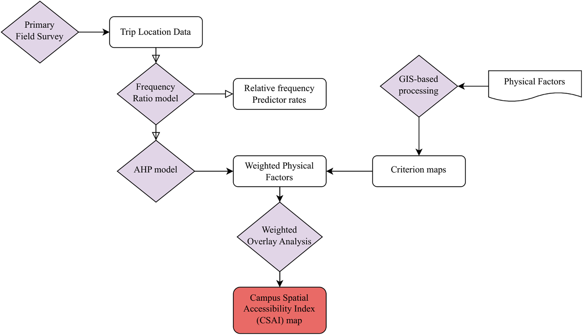
Figure 2: Methodology workflow

3.1 Identifying Physical Factors Influencing Campus Spatial Accessibility Index (CSAI)

Based on a literature review from previous journals, the parameters and methods used for this study were determined. The physical factors used in this study are Slope, Elevation, Building Density, Population Density, Land Use, Intersection Density, Travel Time, and Public Transport Services Area. They had been approved by an expert, also, suitable for the conditions around the university. The factors used in this study are described in Table 1.

3.2 Data Collection

3.2.1 Spatial Data Collection

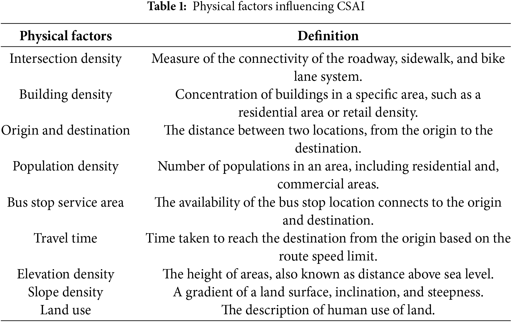
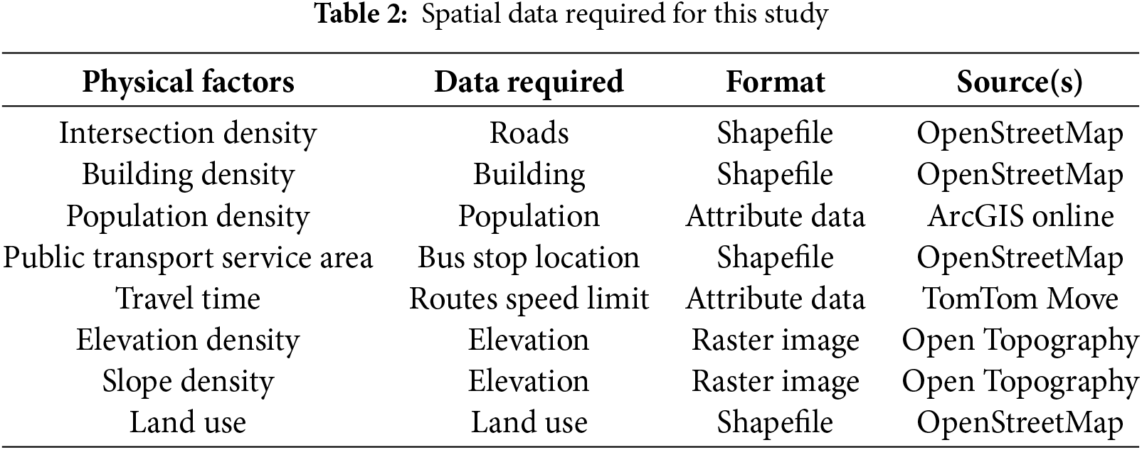
The spatial data needed in this study represent the physical factors influencing the CSAI on the ground. Table 2 summarizes the spatial data needed and the sources of them.

3.2.2 Sample Survey

The sample survey aimed to determine the trip location data among students and to gather information about the types of transportation that are often used among students in the public university in Shah Alam. The primary data from the students are important in order to achieve the objective of this study, which focuses on accessibility on campus. Therefore, from the sample survey, the origin and destination that are always used by the students were also determined.

Trip data locations were obtained by distributing a sample survey to all students in the public university. The main objective of the sample survey is to determine trip location data among the public university’s students. The questions asked in this sample survey are about the most requested transportation used by students to attend class. The respondents for this survey include students who stayed on campus and off campus. In the sample survey, students chose the type of transportation that was used as the main choice for them to attend the class between public transport, including buses that have been provided by the university, or students preferred to attend class by active transport such as walking and cycling. Students also chose the combination of public transport and active transport if they are used to both transportation systems.

In addition, the sample survey also includes the origin and destination point locations of trips. Origin was classified as on-campus colleges or rented houses for off-campus accommodation, meanwhile, destination was classified as a location for students to attend, such as faculty buildings in the public university, commercial areas located at Section 7, Section 2, Section 3, Section 15, and Section 16. The questions that were asked were to find out the destination of demand from students and the type of transportation that students usually use to get to a certain place.

In this study, the respondents were among the public university’s students, and the population on this campus is large. Therefore, the calculation of sample size is to determine the average number of students on the campus, including the number of students who did not answer the sample survey. In 2019, the population of the public university’s students was recorded as 160,957, and this number was used to calculate the sample size. With the larger number of students in the public university, the minimum number of respondents required is at the 95% confidence level. The assumption of confidence level with a normal distribution due to the response of a large population size [19].

The equation was used to calculate the Sample Size of respondent from sample survey where n is the minimum sample size, z is z-statistic of given confidence level, which is the value of confidence level for 95% is 1.96 according to z-statistic table, p is a standard deviation, e is margin of error which is 0.05 and N is population size, 160,957 students in the public university in 2019. Based on the calculation using Eq. (1), the number of respondents needed for primary data collection was 384. However, during this study, 394 respondents answered this sample survey.

3.3 Criterion Weightage Calculation Using FR-AHP Methods

3.3.1 Trip Location Data

The data that has been collected from the sample survey distribution were the mode of transportation used by students, the number of students who use public transport or active transport, as well as the number of students who use a combination of active and public transport. According to the sample survey that has been distributed, students have given information about the location of origin and destination that are most visited by students. The percentage of transportation type used by students in the public university in Shah Alam is 57.9% went to their destination by their own transportation, such as car and motorcycle, 23.4% used public transportation, 13.7% of students used buses, and the remaining 3.3% chose E-Hailing.

3.3.2 Frequency of Trips Using Frequency Ratio (FR)

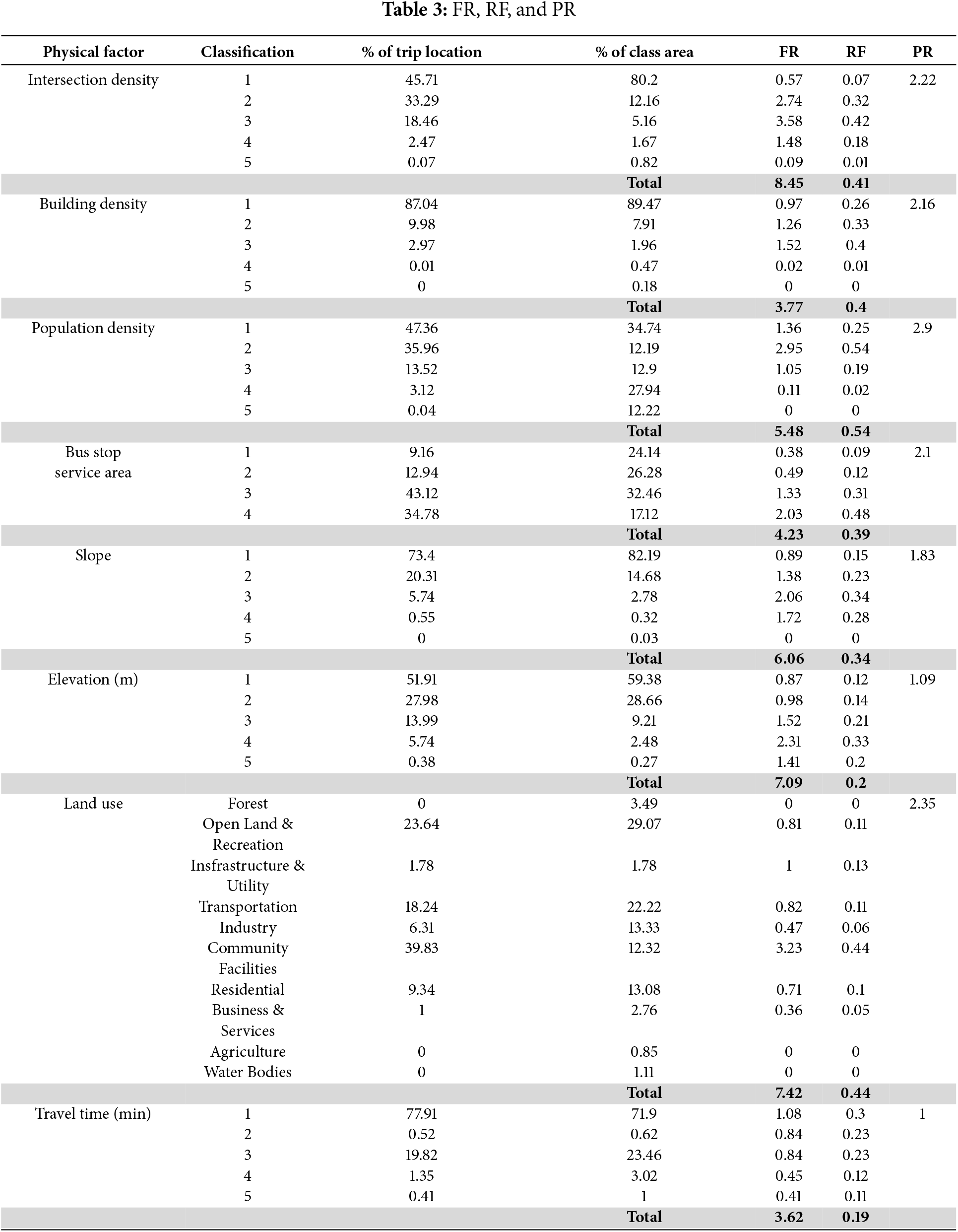
In this study, FR was used to determine the relationship between trip location and Physical Factors. Thus, the trip location can be the dependent variable while Physical Factors are independent variables. The bivariate statistical model FR was used to diagnose the relationship between Physical Factors and active and public transport accessibility. Firstly, the percentage frequency of trip location and the percentage of class area for each different factor class under the selected Physical Factor were calculated. The percentage of trip location has been determined by calculating the number of trips for each destination (study area) and each class for each Physical Factor. Then, the percentage for trip location for each Physical Factor was calculated by dividing the total number of trips for each destination in each class. Next, the percentage of class area was calculated by multiplying the number of cells for each destination area by the size of the cell area. The percentage of the trip location and class area for each Physical Factor has been shown in Table 3. The calculation of FR for a single conditioning factor can be calculated by referring to the Eq. (1) [35].

FR=(Npix(SXi)∑i=1mSXi)(Npix(Xj)∑j=1nNpix(Xj))where:Npix(SXi)=Number of pixels in class i of the factor XNpix(Xj)=Number of pixels within the factorXjm andn=Number of classes in factorXiin the study area(1)

To calculate the probability of the index, the probability can be calculated by referring to Eq. (2).

FPI=∑j=1nFR(2)

3.3.3 Relative Frequency (RF)

As a next step, FRs were normalized in the range of probability values as RF. The proportion of FR value in a factor class of a variable was compared to the total FR of that variable, which is called the RF, and was calculated using Eq. (3).

RF=FR of a factor class∑FR of all factor classes(3)

The value of RF was obtained by dividing the value FR of each class by the summation of FR for all factor classes. For example, the value of FR for population density factors has been obtained for each classification using Eq. (1). To calculate the RF value for population density, divide the FR value of each classification in population density by the total sum of FR values in population density. This calculation will be repeated for the next classification in population density. Eq. (3) were also used to calculate the RF value for other Physical Factors. In combination with FR-AHP, the relative importance of each class of factor will be calculated using Eq. (5). In Eq. (4), FR will represent the value of relative frequency and FRij will represent a value of frequency ratio.

RF=FRij∑FRi(4)

RF=(RFimax−RFimin)(RFimax−RFimin)min(5)

3.3.4 Predictor Rate (PR)

The weightage value used in this study was provided according to the PR values for each Physical Factor. The PR value has been calculated by using Eq. (6). The calculation of PR was calculated to consider any mutual interrelationship among the independent variables. PR was calculated by dividing the difference between the maximum ratio and the minimum ratio of the RF value by the minimum difference among all Physical Factors. For example, to calculate the PR value for the population density factor, the maximum RF value for the population density minus the minimum RF value for the population density factor, the answer will be divided by the minimum summation value of RF. Referring to Table 3, the maximum value of RF is 0.54 minus the minimum value, 0.00. Then, the answer needs to be divided by the minimum difference between the maximum and minimum among all environment factors, which is 0.19, the summation of the RF value of the Travel Time factor. The PR values were used to calculate the weightage for each Physical Factor by using the AHP method.

Followed by the RF equation, the PR for each factor will be calculated using Eq. (6), where FRimax will represent the maximum relative frequency of factor i, FRimin will represent the minimum relative frequency of factor i, and (RFmax−RFmin) will represent the minimum difference between the maximum and minimum relative frequencies for all factors used. For the combination of FR-AHP, the weightage value of PR will be used to calculate the AHP method by using a pairwise matrix.

PR=RFmax−RFmin(RFmax−RFmin)min(6)

Generally, the AHP method, using a pairwise comparison matrix, is dependent on expert judgments [28]. In this study, the AHP method, using a pairwise comparison matrix, was used in determining the weightage value for each parameter, using the PR value obtained from Eq. (7). After obtaining both FR and RF values, the variable-wise values that have been obtained previously will be organized in a row and a column to create a pairwise comparison matrix. The equation for the pairwise comparison matrix is shown in Eq. (7).

Aij=[PR1PR1…PRiPRj………PR1PR1…PRiPRj]=[a11…a1j………ai1…aij](7)

From Eq. (7), Aij represents a pairwise comparison matrix with i is the number of rows and j is the number of columns. However, aij is represented as the entry column of matrix A, with the probability index of ensembled FR-AHP estimated in the range of probability values (0–1), and will divide each entry of the matrix A by the respective column total.

Then, the value of Consistency Ratio (CR) was determined using Eq. (8) to indicate the probability of the randomly generated judgment matrix. In Eq. (8), CR is a Consistency Ratio, CI is the consistency index, and RI is the average of the resulting consistency index [28]. To determine CI, Eq. (9) were used where λmax is the largest principal eigenvalue of the matrix.

CR=CIRI(8)

CI=(CI=(λmax−n)/(n−1)(9)

3.3.5 Pairwise Comparison Matrix

AHP is an MCDA weighing method that can be used to determine the main alternative decisions by comparing the decision of criteria and Physical Factor [19]. AHP was used to determine the relative significance of different Physical Factors in combination with the FR method. To use AHP technique, the variable-wise obtained PR values were organized into matrix form, with a rows and columns, Eq. (5).

The pairwise comparison matrix is used to calculate the weightage value for each Physical Factor using PR values. The matrix above consists of Aij, representing a pairwise comparison matrix with i rows and j columns, where aij is represented as the entry in column of matrix A, as shown in Table 4. The probability index of the FR-AHP value was estimated and normalized in the range of probability values (0–1).

As there are eight (8) Physical Factors used to measure the influences on spatial accessibility, the size of the pairwise comparison matrix was 8 × 8. The PR value of each factor was divided among them, followed by the value that was organized into matrix form. In the end, the weightage for each factor was derived. These values were used to determine CSAI by using GIS.

3.3.6 Consistency Ratio (CR) & Consistency Index (CI)

The value of CR can be calculated by dividing CI by RI values. RI values were determined based on the Random consistency index for a matrix size of 8, which is 1.41. This technique is important to derive the priorities through the Eigenvector from the pairwise comparison matrix and also to measure the consistency weight for each Physical Factor. Table 5 shows the consistency of the calculation.

3.3.7 Campus Spatial Accessibility Index (CSAI)

Lastly, the value of CSAI was measured using a weightage value that was obtained from the FR-AHP calculation. The CSAI was measured using a GIS technique based on the following Eq. (10) that shows the formula to calculate the transport accessibility index, where PRi is the predictor rate of the ith variable, meanwhile RFi is the relative frequency of the ith variable, and n is the total number of variables.

CSAI=∑i=1n(PRiRFi)(10)

3.4 Modelling Campus Spatial Accessibility Index (CSAI)

This process aims to measure the CSAI from spatial data editing to processing spatial data to produce CSAI using GIS techniques. In this study, spatial data editing was started after secondary data collection had been made. Data preparation included data cleaning and clipping. Data cleaning was done by importing all related data required for this study, such as Study Area Sections in Shah Alam, Type of Buildings, Type of Routes, Locations of Public Transport Areas, and Land Use Areas. Meanwhile, data clipping is involved with layers located around study areas only. All Physical Factors layers have been clipped based on the study area boundaries to ensure all processing will be done on the correct areas.

Next, the preparation of the criterion map included GIS processing such as projection, rasterization, density, and reclassification. All Physical Factors must be in the same projection to ensure the analysis can run smoothly and the accessibility will be located at the same places. To measure CSAI using GIS, model builder was used to run WOA for All Physical Factor at the same time. All criterion maps that have been created were used as parameters to determine the best CSAI around the study area in Shah Alam. Lastly, the visualization was done to represent CSAI into a map with five (5) classes. The spatial editing and processing were done using ArcMap software.

The criterion maps produced are shown in Fig. 3. Each criterion map represents a different Physical Factor. These maps were used to determine CSAI. Firstly, all Physical Factor was converted into the same projection, which is in the projected coordinate system WGS 1984. The projected coordinate system was chosen to enable the rasterization process for each layer. After rasterization, GIS processing was done for Building Density, Intersection Density, Population Density, Service Area, Slope, Elevation, Land Use, and Travel Time. Modelling CSAI with WOA.

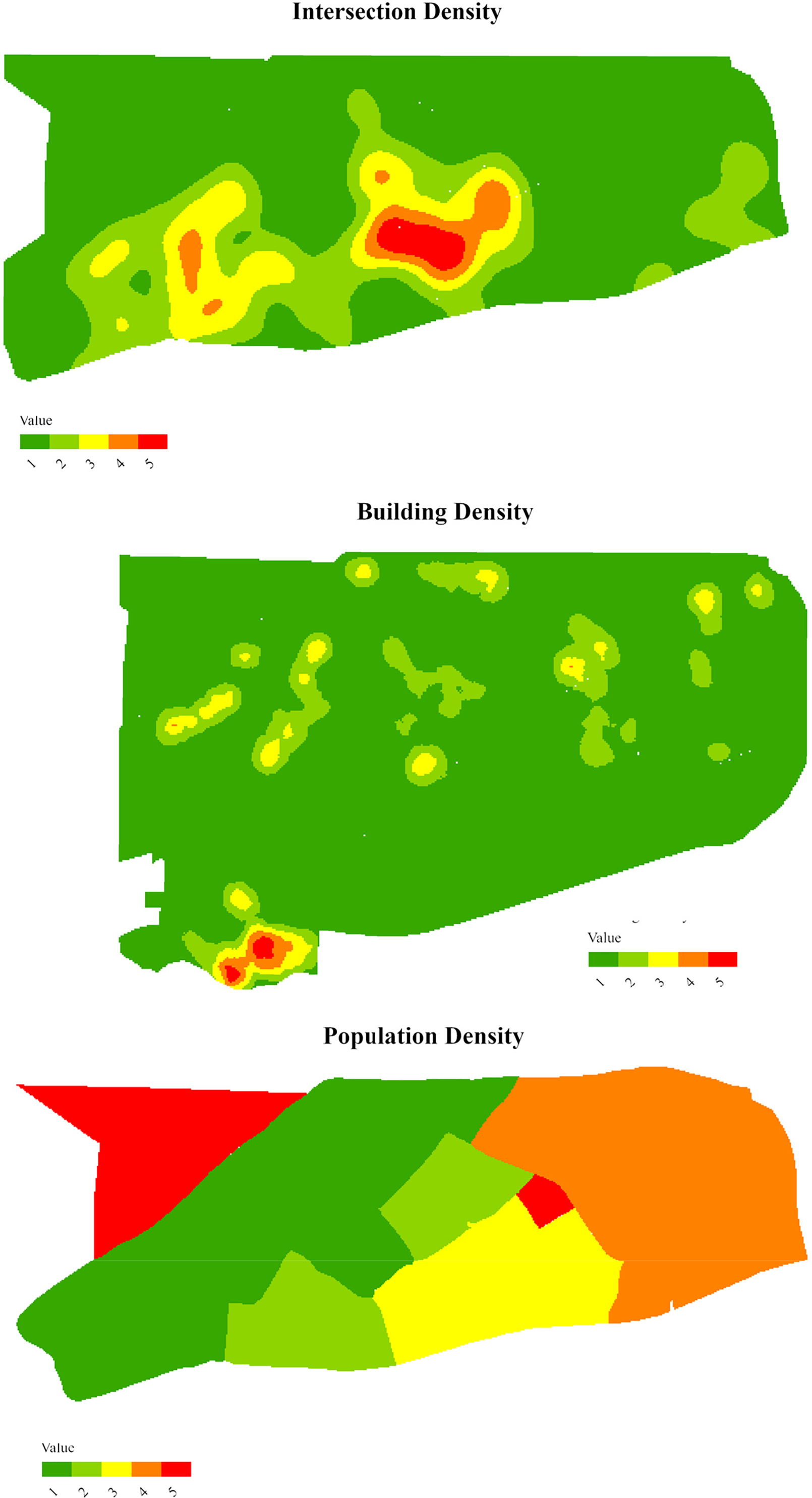
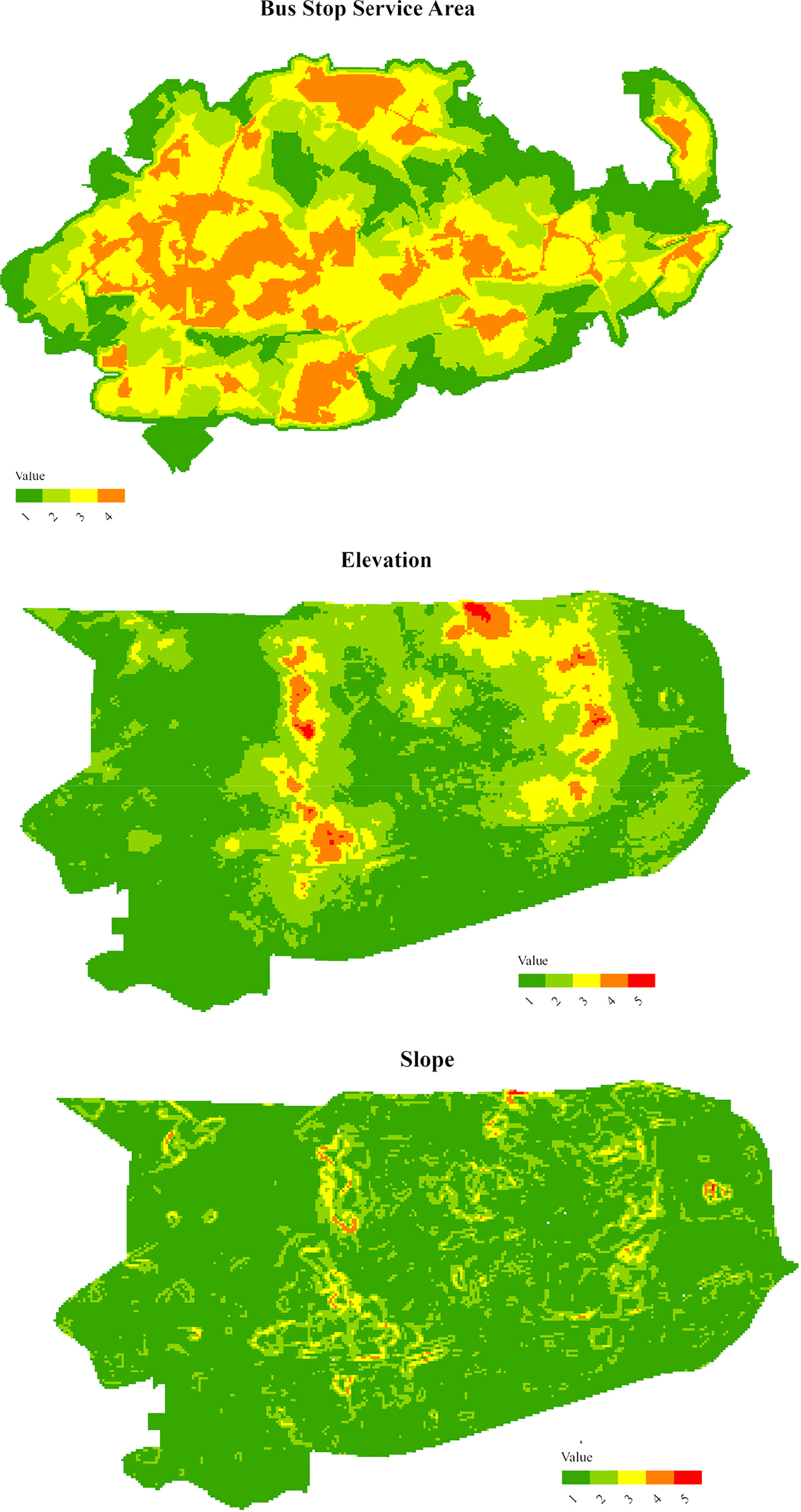
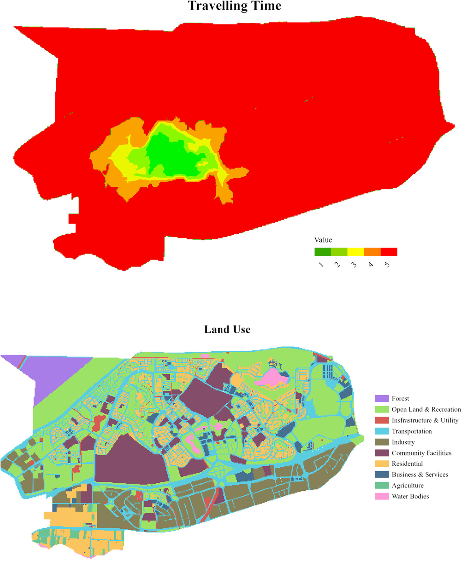
Figure 3: Criterion maps of the factors influencing CSAI

After producing a Criterion Map for each Physical Factor, the CSAI was modelled by using WOA. As the process is lengthy and requires several geoprocessing tasks to be included, automation in GIS was used. This is to reduce any errors or mistakes in the processing since there will be an output from a different task that can be input for the following task. Thus, Modelbuilder was used. In this study, each Physical Factor has been imported into Modelbuilder as shown in Fig. 4. Then, the weighted overlay tool was inserted into the same model and chained together with each Physical Factor. The model was run by inserting the weightage values for each Physical Factor that has been calculated using the FR-AHP method, shown in Table 3. Each class has been classified into 5 classes from Class 1 to Class 5. The scale value of each class for each Physical Factor was set according to a suitable scale value for accessibility. Scale value of 1 will represent Very Low Accessibility, scale value of 2 representing Low Accessibility, scale value of 3 representing Moderate Accessibility, scale value of 4 representing High Accessibility, and scale value of 5 representing High Level Accessibility.

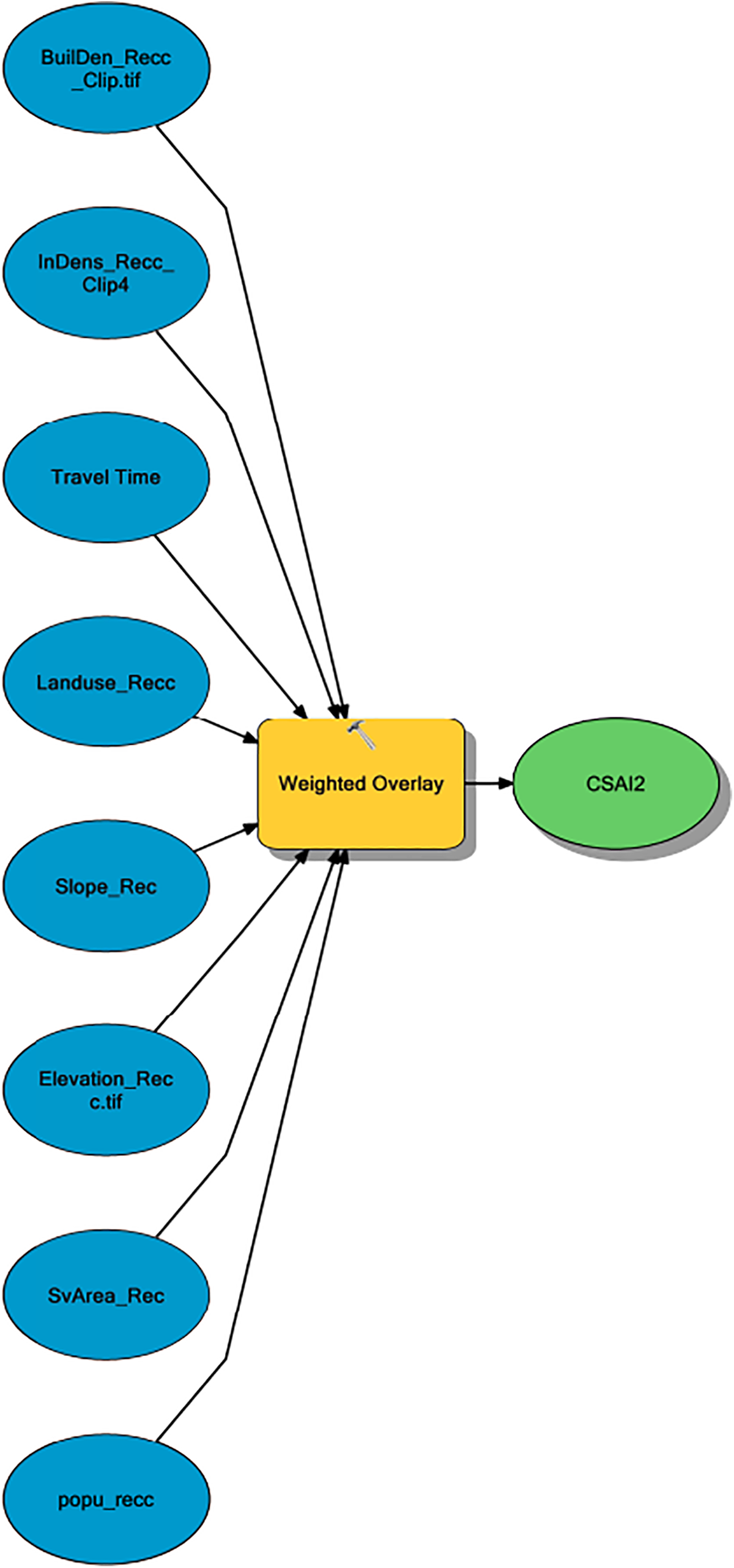
Figure 4: Modelbuilder in ArcGIS to derive CSAI

3.5 Analysis

The final output for this study is CSAI, which has been derived by using WOA. The analysis was chosen to determine the influences of eight Physical Factors on accessibility around the public university in Shah Alam. There were eight (8) Physical Factors that were overlaid together in one study area with a weightage value for each factor. The weightage value has been obtained by previous FR-AHP calculations. The CSAI has been classified into five classes, starting with high accessibility areas in Class 1 and the lowest accessibility areas in Class 5. The accessibility areas have been influenced by all Physical Factors, and areas located in Class 1 can be defined as an area with the best accessibility. Other than that, the accessibility has also been influenced by the number of Trip locations that have been answered by 393 students from the public university. The areas with no Trip Location data remain with no data accessibility in those areas.

4  Results and Discussion

4.1 Weightage of Physical Factors

The weightage of each Physical Factor (Table 6) influences the CSAI. The Physical Factor that most influences accessibility around campus is Population Density with 0.19 values, followed by Land Use 0.15, Intersection Density 0.14, and Building Density 0.14. The Travel Time Physical Factor is the lowest factor affecting accessibility in this area, with a value of 0.06. The difference between the most influential and the least influential Physical Factor is 0.013, which represents a huge gap in influence between Population Density and Travel Time. Population Density is categorized as having the highest influence on transportation accessibility because an area with a high population will increase the traffic congestion in those areas. The increase in Population Density will lead to an increase in Road Density. Hence, the Intersection Density is categorized as the third most influential factor of accessibility, followed by Building Density.

The moderate influence of Physical Factor is a Bus Stop Service Area with 0.13. The Bus Stop Service Area was analyzed based on four (4) different distances, which are 400, 800, 1200, and 1600 m. The distance is an approachable distance that can be reached by students. The physical Factor with the minimum influence for transportation accessibility is Slope Density with 0.12. An area with a slope will affect the accessibility of transportation.

The value of Elevation Density is only 0.07. The Physical Factor of Elevation Density can be categorized as having a low influence on accessibility. An area with a higher degree of slope and elevation will have low accessibility to the transportation system. Travel Time factor is the factor with the least influence on accessibility around the campus, with 0.06. The time required for students to travel 800 m is only 10 min from the origin, the university. Whereas, for 1.2, 1.6, 2 km, and areas with more than 2 km, it only required 15, 20, 25, and more than 25 min to reach areas more than 2 km from the origin.

4.2 Campus Spatial Accessibility Index

The estimated RF and PR were used to create the CSAI map (Fig. 5). The indices were classified into five (5) categories by using Natural Breaks (Jenks). The classification method was chosen due to its ability to determine natural grouping in the data that is unevenly distributed by minimizing variance within the classes and maximizing variance between them. The categories used in this study are Very Low, Low, Moderate, High, and Very High, and each category represents the level of active and public transport accessibility. The CSAI map also shows the level of accessibility according to the classes. This map visualizes the CSAI index that has been obtained using the FR-AHP method.

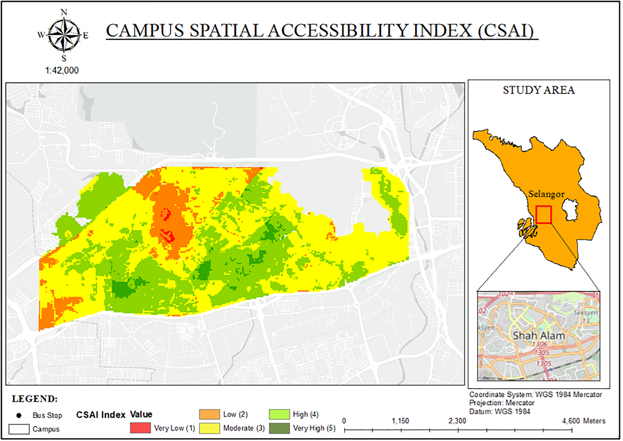
Figure 5: Campus spatial accessibility index (CSAI) map

The findings of this study are 2.7% of the study area with Very High CSAI, 35.34% of the study area with High CSAI, and the highest CSAI was 51.37% of the study area with Moderate CSAI. While the lowest index, Low Accessibility, was located in a hilly residential area in Section 8 and Section 7, with 10.29% of the study area, and 0.31% of the study area with Very Low CSAI. This shows that the area around the public university has a good level of accessibility because more than 50% of the study area has a high index status between Moderate, High, and Very High CSAI. Therefore, the residential area around this area has an advantage to live in because it has high access to nearby transportation, either by using public transport or active mobility.

To validate the efficiency of using the ensemble of FR and AHP in measuring the CSAI, a model derived with only FR was used. FR values themselves could be treated as weightage in GIS modelling. Hence, this study used the FR values calculated for each factor in the Weighted Overlay Analysis to derive the CSAI as shown in Fig. 6. As a result, although some areas recorded similar CSAI, there are notably several differences in the CSAI derived using FR-AHP and only FR.

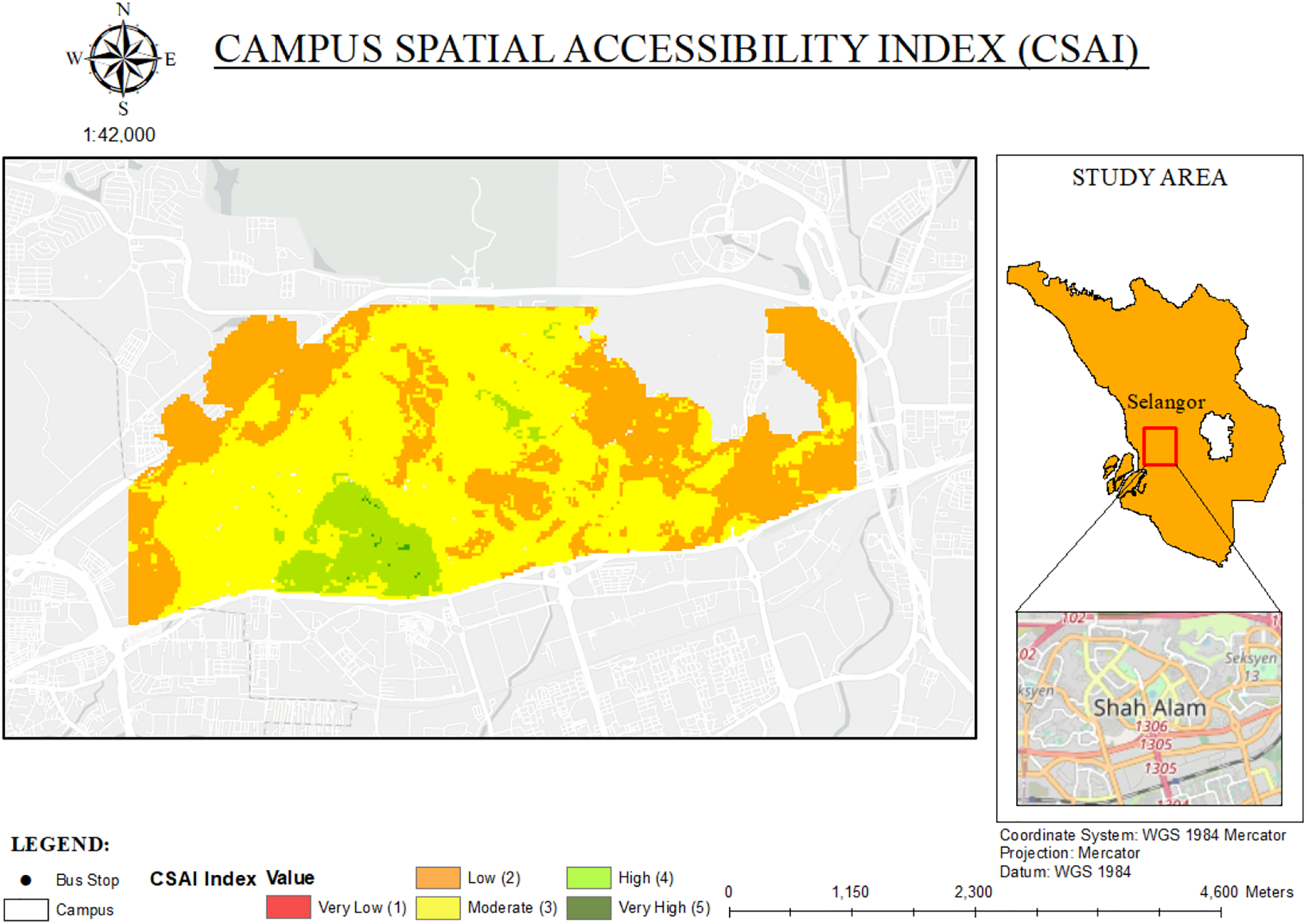
Figure 6: Campus spatial accessibility index (CSAI) map derived using FR

First, there are no Very Low CSAI when derived by using FR only. Secondly, the coverage areas for each class. Table 7 summarizes the differences in the percentage number of pixels with each CSAI class for both the FR-derived model and the FR-AHP ones. Except for the Very Low, Moderate, and Very High classes, there are vast differences between the other two classes. Although the CSAI of most areas is different by one (1) scale class when deriving with different models, there are areas with high CSAI for both the FR and FR-AHP models, which is Section 1, which is the university compound.

It is challenging to decide which of the two methods is more accurate, as there is yet to be a standard model used in Malaysia to measure spatial accessibility for a campus. Different studies used different parameters and even models. However, this study attempted to validate the results with field verification and relating the results with the demand for accessibility, as one of the Factors that influence the CSAI is population.

Table 8 shows the population in areas with Moderate CSAI, High CSAI, and Very High CSAI. These sections are considered an area with good accessibility. Fig. 7 shows the correlation between population density and CSAI. It is revealed that the two have a positive correlation with a coefficient of 0.2297. In this study, Section 1 has been determined as an area with Very High CSAI with a population of 516.54. This Section is also the nearest Section around the university where students can consider finding a rental house to attend classes on campus. An area with a high population will have higher accessibility to the nearest public transportation as one of the facilities. Other than that, in Section 2, there is also a residential college for the students, which is Meranti College. One of the facilities provided by the university to students is free bus services. This area is also close to other facilities such as a food court, printing services, and a bus stop. Therefore, students can consider Section 2 as one of the best options for residential areas during their studies due to its high accessibility and proximity to various facilities.

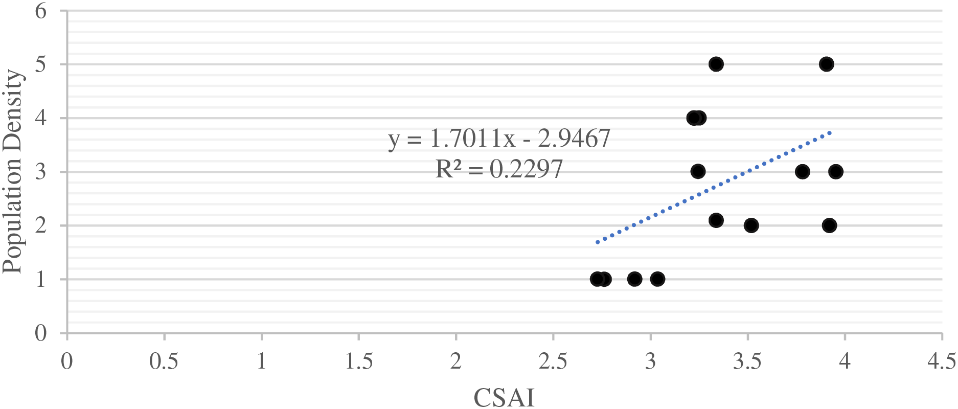
Figure 7: Correlation between CSAI and population density

Next is an area with High CSAI, which was located at Section 4, Section 14, and Section 1. Section 4 is a residential area with the nearest bus stop facilities. In this study, Section 4 has been classified as High CSAI due to the high density of buildings and high road intersections in these areas. Fig. 8 shows the study area with Road Intersection with Building Density. Fig. 9 shows the correlation of CSAI with the Intersection Density. It is revealed that the correlation between the two is positive with a coefficient of 0.2337. Higher Intersection Density could improve accessibility as the road would be more connected, creating a more walkable street network, which is beneficial for pedestrians and public transport users, as this study intended to measure.

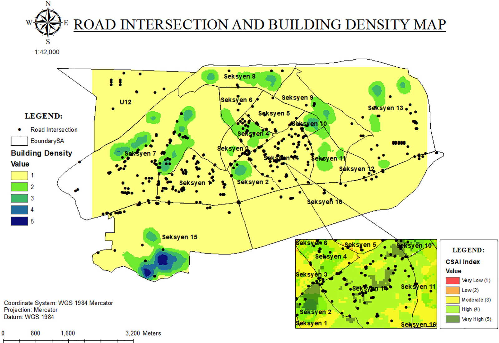
Figure 8: Road intersection and building density map

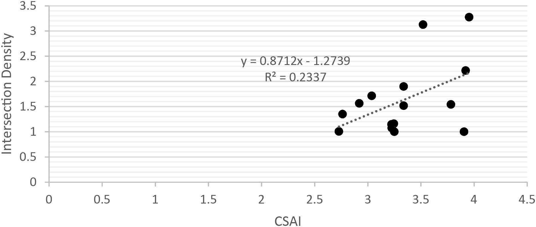
Figure 9: Correlation between CSAI and intersection density

High building density representing a residential building in Section 4, and the intersection density shows there is an access for students to use public transportation, as well as active mobility from their origin to the destination. Section 14 is an area with various facilities such as hospitals, banks, and government buildings, as well as various attractions such as Shah Alam Lake, shopping malls, and others. With the availability of various facilities and attractions in this area, students can also find nearby residential areas in Section 14. Next, Section 1 has also been defined as areas with High CSAI. Based on a survey conducted among the students, there were 12.27% of % number of trips taken to Section 1. Additionally, the university was also located in Section 1 and has good accessibility on the campus.

Areas with Moderate CSAI can also be used as searching areas for rental houses. This is because, in this study, the highest CSAI is Moderate with 51.37% of the study area. The area with Moderate CSAI also has a high population, such as Section 7 with 4355.09. A high population can provide high accessibility due to high transportation in Section 7. Other than that, Section 7 is also the most rented area by the students because it is one of the nearest sections to the university. There is also a free bus service by the state government, as well as buses provided by the university, taking the roads in Section 7 as the main bus route to the campus. Therefore, Section 7 can be categorized as a suitable area for students to rent a house because it has a bus route that will enter the campus.

Other than Section 7, there are also some sections that have been defined as Moderate accessibility, which are Section 12, Section 13, Section 9, and Section 8. All of this area was defined as Moderate CSAI due to the influence of the Physical Factor used in this study. Students from the university can also consider these Sections as areas to build rental houses; however, it might not be preferable to students who do not have their own transportation because the distance is quite far from the the university. Even so, students can also consider the house rental prices in these sections because they might be lower than the house rental prices in Section 7. There are many factors that can be considered to find a rental house for students, and accessibility is one of the factors that need to be considered.

5  Conclusions

The integration of FR-AHP in GIS successfully models the CSAI. The model was validated by analysing the influence of eight (8) Physical Factors towards the CSAI in this study, as they are used to determine areas that give good accessibility. By using the FR-AHP concept, the number of trips taken by students based on the survey questionnaire helped in measuring the influence of accessibility around the university. From the number of respondents, the origin and destination of students have been obtained and are being used to measure the CSAI influenced by Physical Factors used in this study. The CSAI was evaluated by a questionnaire distributed among students to obtain the number of trip locations. The determination of the most influential Physical Factor was made by using eight (8) factors and was analyzed in this chapter. Five classes of accessibility have been found by using WOA, which include Very Low, Low, Moderate, High, and Very High CSAI. At the end, to have a better visualization of areas with high accessibility, a CSAI map was produced. The areas with Very High, High, and Moderate CSAI can be proposed as areas to search for house rentals around the university. This study, however, only focuses on the area around one public university in Shah Alam, Malaysia. In the future, it is recommended to derive the CSAI around other universities in Shah Alam, as well as other areas for comparison purposes.

Acknowledgement: The authors would like to thank Universiti Teknologi MARA for supporting this study and the Land Surveyors Board Malaysia for funding this paper.

Funding Statement: The authors received funding from the Land Surveyors Board Malaysia for this study.

Author Contributions: The authors confirm contribution to the paper as follows: study conception and design: Nur Sabrina Jamal, Nabilah Naharudin; data collection: Nur Sabrina Jamal; analysis and interpretation of results: Nur Sabrina Jamal, Nabilah Naharudin; draft manuscript preparation: Nur Sabrina Jamal, Nabilah Naharudin. All authors reviewed the results and approved the final version of the manuscript.

Availability of Data and Materials: The data is confidential as it is obtained only for the purpose of this study and cannot be disclosed.

Ethics Approval: Not applicable.

Conflicts of Interest: The authors declare no conflicts of interest to report regarding the present study.

References

1. Bokhari A, Sharifi F. Public transport and subjective well-being in the just city: a scoping review. J Transp Health. 2022;25(1):101372. doi:10.1016/j.jth.2022.101372. [Google Scholar] [CrossRef]

2. Manaugh K, Waygood EO, Pellecuer L. Public health, active transport, and land use. In: Handbook on transport and land use. Cheltenham, UK: Edward Elgar Publishing; 2023. p. 332–49 doi:10.4337/9781800370258.00027. [Google Scholar] [CrossRef]

3. Park J, Goldberg DW. A review of recent spatial accessibility studies that benefitted from advanced geospatial information: multimodal transportation and spatiotemporal disaggregation. ISPRS Int J Geo Inf. 2021;10(8):532. doi:10.3390/ijgi10080532. [Google Scholar] [CrossRef]

4. Cook S, Stevenson L, Aldred R, Kendall M, Cohen T. More than walking and cycling: what is ‘active travel’? Transp Policy. 2022;126(5):151–61. doi:10.1016/j.tranpol.2022.07.015. [Google Scholar] [CrossRef]

5. Mirzahossein H, Rassafi AA, Jamali Z, Guzik R, Severino A, Arena F. Active transport network design based on transit-oriented development and complete street approach: finding the potential in Qazvin. Infrastructures. 2022;7(2):23. doi:10.3390/infrastructures7020023. [Google Scholar] [CrossRef]

6. Mohd Yusoff Z, Aziz IS, Naharudin N, Abdul Rasam AR, Ling OHL, Nasrudin NA. Mobility and proximity coefficient to high-traffic volume in daily school operations. Plan Malays. 2022;20(2):321–32. doi:10.21837/pm.v20i21.1116. [Google Scholar] [CrossRef]

7. Olayode IO, Chau HW, Jamei E. Barriers affecting promotion of active transportation: a study on pedestrian and bicycle network connectivity in Melbourne’s west. Land. 2025;14(1):47. doi:10.3390/land14010047. [Google Scholar] [CrossRef]

8. Baobeid A, Koç M, Al-Ghamdi SG. Walkability and its relationships with health, sustainability, and livability: elements of physical environment and evaluation frameworks. Front Built Environ. 2021;7:721218. doi:10.3389/fbuil.2021.721218. [Google Scholar] [CrossRef]

9. Ceder A. Urban mobility and public transport: future perspectives and review. Int J Urban Sci. 2021;25(4):455–79. doi:10.1080/12265934.2020.1799846. [Google Scholar] [CrossRef]

10. Ruslan N, Naharudin N, Salleh AH, Abdul Halim M, Abd Latif Z. Spatial walkability index (SWI) of pedestrian access to rail transit station in Kuala Lumpur city center. Plan Malays. 2023;21(5):237–52. doi:10.21837/pm.v21i29.1368. [Google Scholar] [CrossRef]

11. Hassan M, Mahin HD, Ahmed F, Hassan MM, Rahaman A, Abdullah M. Assessing public transit network efficiency and accessibility in Johor Bahru and Penang, Malaysia: a data-driven approach. Results Eng. 2025;27(9):106126. doi:10.1016/j.rineng.2025.106126. [Google Scholar] [CrossRef]

12. Olfindo R. Transport accessibility, residential satisfaction, and moving intention in a context of limited travel mode choice. Transp Res Part A Policy Pract. 2021;145(3):153–66. doi:10.1016/j.tra.2021.01.012. [Google Scholar] [CrossRef]

13. Logan TM, Hobbs MH, Conrow LC, Reid NL, Young RA, Anderson MJ. The x-minute city: measuring the 10, 15, 20-minute city and an evaluation of its use for sustainable urban design. Cities. 2022;131(7):103924. doi:10.1016/j.cities.2022.103924. [Google Scholar] [CrossRef]

14. Sun C, Cheng J, Lin A, Peng M. Gated university campus and its implications for socio-spatial inequality: evidence from students’ accessibility to local public transport. Habitat Int. 2018;80:11–27. doi:10.1016/j.habitatint.2018.08.008. [Google Scholar] [CrossRef]

15. Ferrari G, Drenowatz C, Kovalskys I, Gómez G, Rigotti A, Cortés LY, et al. Walking and cycling, as active transportation, and obesity factors in adolescents from eight countries. BMC Pediatr. 2022;22(1):510. doi:10.1186/s12887-022-03577-8. [Google Scholar] [PubMed] [CrossRef]

16. Hansmann KJ, Grabow M, McAndrews C. Health equity and active transportation: a scoping review of active transportation interventions and their impacts on health equity. J Transp Health. 2022;25(2):101346. doi:10.1016/j.jth.2022.101346. [Google Scholar] [CrossRef]

17. Cho S, Choi K. Transport accessibility and economic growth: implications for sustainable transport infrastructure investments. Int J Sustain Transp. 2021;15(8):641–52. doi:10.1080/15568318.2020.1774946. [Google Scholar] [CrossRef]

18. Inturri G, Giuffrida N, Le Pira M, Fazio M, Ignaccolo M. Linking public transport user satisfaction with service accessibility for sustainable mobility planning. ISPRS Int J Geo Inf. 2021;10(4):235. doi:10.3390/ijgi10040235. [Google Scholar] [CrossRef]

19. Zannat KE, Adnan MSG, Dewan A. A GIS-based approach to evaluating environmental influences on active and public transport accessibility of university students. J Urban Manag. 2020;9(3):331–46. doi:10.1016/j.jum.2020.06.001. [Google Scholar] [CrossRef]

20. Tiran J, Razpotnik Visković N, Gabrovec M, Koblar S. A spatial analysis of public transport accessibility in Slovenia. Urbani Izziv. 2022;33(1):105–21. doi:10.5379/urbani-izziv-en-2022-33-01-04. [Google Scholar] [CrossRef]

21. Rodrigue JP. A.4—transportation and accessibility|The geography of transport systems [Internet]. [cited 2025 Jan 1]. Available from: https://transportgeography.org/contents/methods/transportation-accessibility/. [Google Scholar]

22. Vecchio G, Martens K. Accessibility and the capabilities approach: a review of the literature and proposal for conceptual advancements. Transp Rev. 2021;41(6):833–54. doi:10.1080/01441647.2021.1931551. [Google Scholar] [CrossRef]

23. Tao Z, Cheng Y, Zheng Q, Li G. Measuring spatial accessibility to healthcare services with constraint of administrative boundary: a case study of Yanqing District, Beijing. China Int J Equity Health. 2018;17(1):7. doi:10.1186/s12939-018-0720-5. [Google Scholar] [PubMed] [CrossRef]

24. Kanuganti S, Sarkar AK, Singh AP. Quantifying accessibility to health care using two-step floating catchment area method (2SFCAa case study in Rajasthan. Transp Res Procedia. 2016;17(3):391–9. doi:10.1016/j.trpro.2016.11.080. [Google Scholar] [CrossRef]

25. Lin Y, Wan N, Sheets S, Gong X, Davies A. A multi-modal relative spatial access assessment approach to measure spatial accessibility to primary care providers. Int J Health Geogr. 2018;17(1):33. doi:10.1186/s12942-018-0153-9. [Google Scholar] [PubMed] [CrossRef]

26. Luo W, Wang F. Measures of spatial accessibility to healthcare in a GIS environment: synthesis and a case study in Chicago Region. Environ Plann B Plann Des. 2003;30(6):865–84. doi:10.1068/b29120. [Google Scholar] [PubMed] [CrossRef]

27. Silalahi FES, Pamela, Arifianti Y, Hidayat F. Landslide susceptibility assessment using frequency ratio model in Bogor, West Java, Indonesia. Geosci Lett. 2019;6(1):10. doi:10.1186/s40562-019-0140-4. [Google Scholar] [CrossRef]

28. Meten M, Bhandary NP, Yatabe R. GIS-based frequency ratio and logistic regression modelling for landslide susceptibility mapping of Debre Sina area in central Ethiopia. J Mt Sci. 2015;12(6):1355–72. doi:10.1007/s11629-015-3464-3. [Google Scholar] [CrossRef]

29. Saaty TL. Decision making with the analytic hierarchy process. Int J Serv Sci. 2008;1(1):83. doi:10.1504/ijssci.2008.017590. [Google Scholar] [PubMed] [CrossRef]

30. Malczewski J, Rinner C. Introduction to GIS-MCDA. In: Multicriteria decision analysis in geographic information science. Berlin/Heidelberg, Germany: Springer; 2015. p. 23–54. doi:10.1007/978-3-540-74757-4_2. [Google Scholar] [CrossRef]

31. Saha A, Mandal S, Saha S. Geo-spatial approach-based landslide susceptibility mapping using analytical hierarchical process, frequency ratio, logistic regression and their ensemble methods. SN Appl Sci. 2020;2(10):1647. doi:10.1007/s42452-020-03441-3. [Google Scholar] [CrossRef]

32. Yilmaz OS. Flood hazard susceptibility areas mapping using analytical hierarchical process (AHPfrequency ratio (FR) and AHP-FR ensemble based on geographic information systems (GISa case study for Kastamonu, Türkiye. Acta Geophys. 2022;70(6):2747–69. doi:10.1007/s11600-022-00882-9. [Google Scholar] [CrossRef]

33. Gupta N, Pal SK, Das J. GIS-based evolution and comparisons of landslide susceptibility mapping of the East Sikkim Himalaya. Ann GIS. 2022;28(3):359–84. doi:10.1080/19475683.2022.2040587. [Google Scholar] [CrossRef]

34. Razandi Y, Pourghasemi HR, Neisani NS, Rahmati O. Application of analytical hierarchy process, frequency ratio, and certainty factor models for groundwater potential mapping using GIS. Earth Sci Inform. 2015;8(4):867–83. doi:10.1007/s12145-015-0220-8. [Google Scholar] [CrossRef]

35. Shafapour Tehrany M, Kumar L, Neamah Jebur M, Shabani F. Evaluating the application of the statistical index method in flood susceptibility mapping and its comparison with frequency ratio and logistic regression methods. Geomat Nat Hazards Risk. 2019;10(1):79–101. doi:10.1080/19475705.2018.1506509. [Google Scholar] [CrossRef]