Evaluation of Projected Change in Climate Extreme Events through CMIP6 Models over Omo Gibe River Basin, Ethiopia

1  Introduction

Extreme climate disasters pose an urgent and escalating threat due to global warming [1]. Observational records and climate model simulations consistently demonstrate that anthropogenic climate change is increasing the frequency, intensity, and duration of extreme weather and climate events [2]. In particular, the intensification of severe precipitation has amplified hydro-meteorological hazards, elevating flood risks, disrupting infrastructure, and degrading terrestrial and aquatic ecosystems [3]. Globally, droughts and floods now represent the most frequent and destructive natural disasters, with profound social, economic, and environmental consequences [4,5].

Global Climate Models (GCMs) developed through the Coupled Model Intercomparison Project (CMIP) provide the primary framework for assessing historical and future changes in mean climate and extremes at global to regional scales [6]. These models have been widely applied to evaluate climate variability and shifts in extreme events [7]. Numerous studies report that continued warming is likely to intensify heavy precipitation, heat extremes, and droughts worldwide [8–12]. Considerable research has therefore focused on improving methods to characterize past extremes and to enhance projections using multi-model ensembles, particularly through model intercomparison and regional downscaling approaches [13,14]. For example, comparisons between CMIP3 and CMIP5 ensembles showed that CMIP5 models generally produce more realistic and intense precipitation extremes, whereas temperature extremes exhibit smaller inter-model differences [14]. The results revealed significant variation in precipitation indices, with CMIP5 models generally simulating more intense precipitation extremes that closely align with observational data. In contrast, temperature extremes exhibited less variability across the models. Numerous studies have conducted extensive analyses of projected changes in climate extremes at both global and regional scales, using various stages of the CMIP [15,16]. Building on earlier phases, the latest generation, CMIP6, offers improved process representation and higher spatial resolution, creating new opportunities for more reliable regional assessments [17].

A key objective of CMIP6 is the robust evaluation of historical and future changes in climate extremes and the physical mechanisms driving them [17,18]. Previous assessments using CMIP3 and CMIP5 have examined global precipitation characteristics, including seasonal variability and extreme rainfall [19,20]. Nevertheless, comparatively few studies have addressed extremes at local and basin scales, particularly in regions with complex topography and heterogeneous climate regimes [21]. Such regional analyses are essential for translating global projections into actionable information for water-resource management and disaster-risk reduction.

The Omo–Gibe River Basin (OGRB) in Ethiopia exemplifies a region where climate extremes have critical development implications. The basin hosts a cascade of five major hydropower dams with a combined capacity of about 4914 MW, Gibe I (184 MW), Gibe II (420 MW), Gibe III (1870 MW), and the planned Gibe IV (1472 MW) and Gibe V (560 MW), along with extensive irrigation schemes and sugar industries that support national energy security and livelihoods [22]. Regional projections for Ethiopia and East Africa consistently indicate robust warming throughout the 21st century, typically 1.5°C–2.5°C under intermediate scenarios and exceeding 3°C under high-emission pathways, accompanied by increases in temperature-extreme indices [23]. Although precipitation projections remain more uncertain, many studies suggest intensification of heavy rainfall events and greater seasonal variability, particularly during the main rainy seasons. These trends highlight the need for basin-specific assessments linking climate extremes to hydrological impacts.

Recent studies have increasingly applied CMIP6 model ensembles to assess climate extremes over Ethiopia and broader East Africa, revealing important regional trends and methodological considerations. For example, a multi-model evaluation of 45 CMIP6 simulations found systematic seasonal extreme precipitation biases over Ethiopia and highlighted the need for bias correction before impact assessment [24]. Similarly, trend analyses in the Gidabo watershed demonstrated future increases in heavy rainfall and temperature extremes under SSP2-4.5 and SSP5-8.5, with implications for runoff and watershed management [25]. Other basin-scale studies, such as in the Baro–Akobo system, have combined CMIP6 analysis with hydrological modelling to examine extremes and flood linkage [26]. However, existing studies often rely on a limited number of models or indices, focus on isolated impact pathways, and rarely integrate model-skill assessment, seasonal behaviour, and hydrological responses at sub-basin scales.

Despite its socio-economic importance and climatic complexity, a comprehensive evaluation of climate extremes in the OGRB remains limited. Earlier investigations in parts of the basin have relied exclusively on CMIP5 models and RCP scenarios, without systematic procedures for model selection or use of the newer CMIP6 framework [27,28]. The absence of a consistent, purpose-driven model evaluation constrains confidence in projected changes to water resources and extremes. Incorporating CMIP6 models under Shared Socioeconomic Pathways (SSPs), together with rigorous assessment of their ability to represent regional precipitation processes and convection dynamics, is therefore essential for generating more reliable, location-specific projections.

Addressing these gaps, this study pursues the following objectives: (i) to evaluate the capability of selected CMIP6 models in reproducing observed temperature and precipitation extremes over the Omo–Gibe River Basin; (ii) to quantify future changes in extreme temperature and precipitation indices under SSP2-4.5 and SSP5-8.5 scenarios; and (iii) to assess the hydrological implications of these projected extremes for basin streamflow through the HEC-HMS model. The study aims to improve understanding of how future changes in heavy rainfall, droughts, and temperature extremes may influence water-resource dynamics and climate-risk management within this strategically vital basin.

2  Materials and Methods

2.1 Study Area Description

The Omo-Gibe River Basin (OGRB) plays a crucial role in Ethiopia’s national economy, covering a total area of approximately 79,000 km2, with an average width of 140 km and a length of 550 km. The basin supports various economic activities, including large and small-scale irrigation systems, sugar industries, and major hydropower projects such as the Gibe I, Gibe II, and Gibe III power plants, which are vital for national energy production and water resource management. In addition to the existing Gibe I, Gibe II, and Gibe III hydropower projects, additional dams, including Gibe IV and Gibe V, have been proposed to further enhance Ethiopia’s energy production and water resource management. Beyond its economic and hydropower significance, the OGRB also hosts several untapped ecotourism destinations, offering opportunities for sustainable tourism development and biodiversity conservation. The OGRB is situated between 4°00′ and 9°22′ N latitude and 34°44′ and 38°24′ E longitude. The river originates in the northern highlands and flows southward through diverse landscapes, including lowland areas, before ultimately draining into Lake Turkana at the Ethiopia-Kenya border. Along its course, the basin receives water from numerous minor and major tributaries, contributing to its hydrological significance [29]. The highlands of the Omo-Gibe River Basin (OGRB), located in the far north and northwest of the basin, are characterized by a humid tropical climate, while the southern lowlands experience a hot, dry climate. The basin’s elevation ranges from 235 to 3625 m above sea level, contributing to significant climatic and ecological variability across the region. The precipitation regime in the OGRB varies spatially, with a monomodal rainfall pattern in the northern and central regions and a bimodal pattern in the southern portions of the basin [29]. Annual rainfall distribution also exhibits significant variation, with the extreme southern lowlands receiving approximately 300 mm, while the central and northwestern highlands receive up to 2000 mm. Correspondingly, the average annual temperature ranges from approximately 16°C in the northern highlands to nearly 30°C in the southern lowlands [30]. The primary land use types in the Omo-Gibe River Basin (OGRB) include woodland (30.02%), intensively farmed land (29.82%), bushland (10.06%), forest (8%), grassland (7.45%), and moderately farmed land (7.08%) [31]. The location and main geographic features of the Omo–Gibe River Basin are presented in Fig. 1.

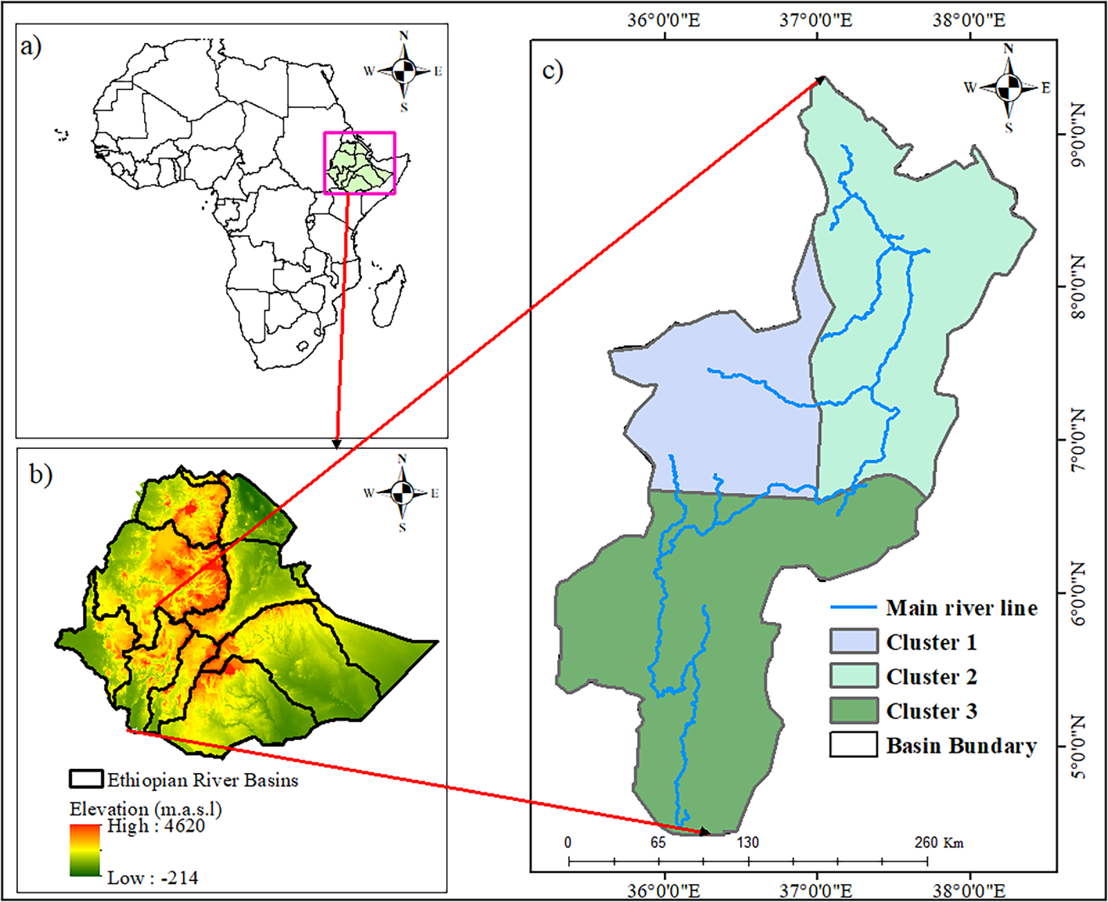
Figure 1: Map showing the location of the research region, (a) Africa map, (b) DEM of major Ethiopian river Basins, and (c) Clusters of the Omo Gibe River Basin [32].

2.2 Data

2.2.1 Observed Data

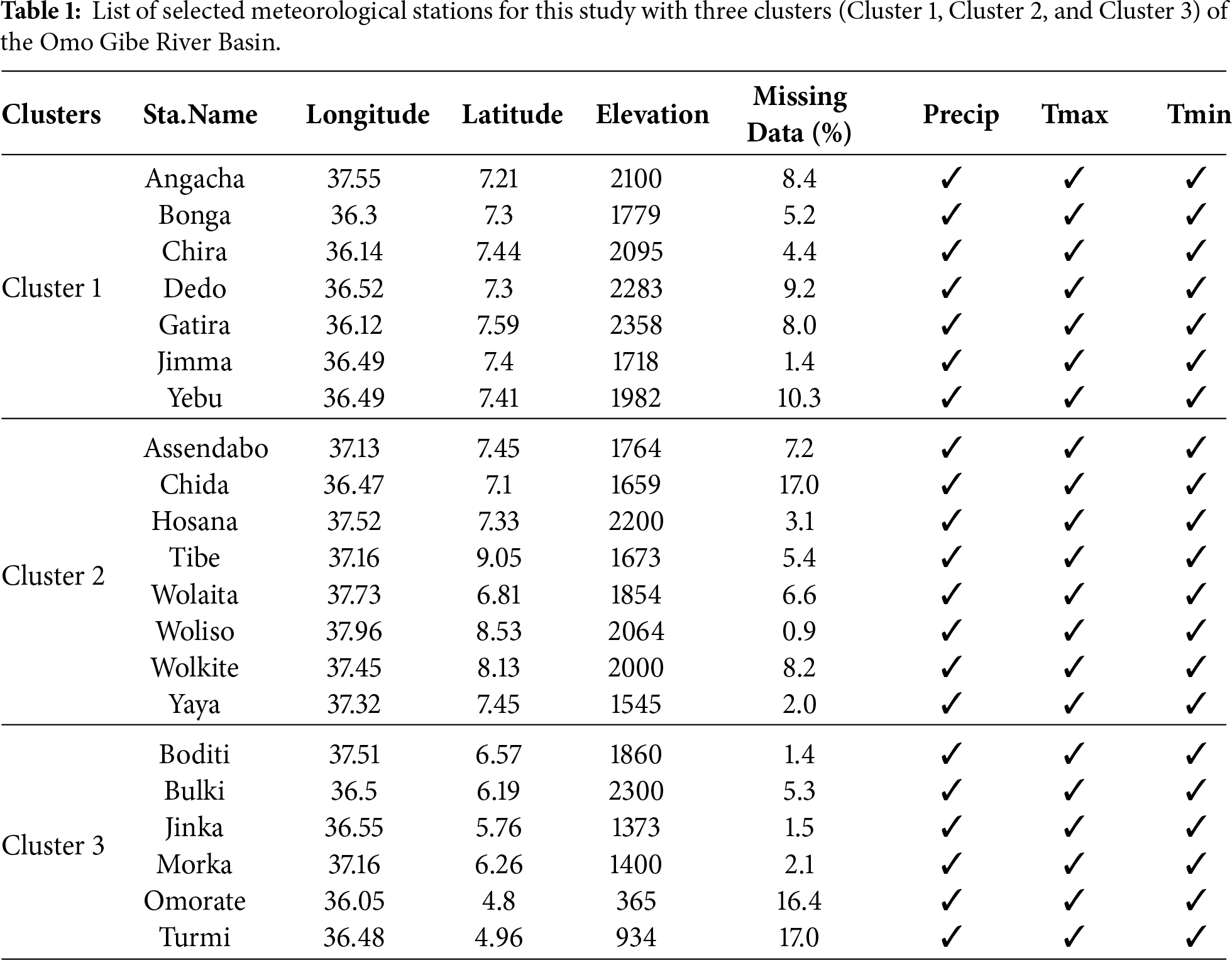
This study employs observed daily precipitation, maximum and minimum temperature data, along with gridded climate datasets provided by the Ethiopian Meteorology Institute (EMI). The dataset spans from 1984 to 2014 and has a spatial resolution of 4 km × 4 km, ensuring comprehensive coverage of the OGRB. The gridded dataset used in this study integrates satellite-derived estimates of temperature and rainfall from the European Organization for the Exploitation of Meteorological Satellites (EUMETSAT) and the U.S. National Aeronautics and Space Administration (NASA), combined with observed station data from the national network operated by the Ethiopian Meteorology Institute (EMI) [33]. This gridded dataset addresses the spatial and temporal gaps in Ethiopia’s national observation data, providing higher data quality for more accurate climate analysis [34]. The daily gridded data was specifically used to compensate for missing station data, particularly in remote or data-sparse regions. By incorporating satellite-derived estimates and ground-based observations, this dataset allows for a more comprehensive and reliable representation of climate patterns across the OGRB. This integration is particularly useful for modelling climate extremes and assessing changes in precipitation and temperature over time, ensuring that the results of the study are robust and well-supported by available data. For this study, data from 21 meteorological stations were utilized, selected based on the availability of long-term records spanning more than 30 years. The stations were chosen to ensure a broad geographic coverage across the OGRB, representing different climate zones and capturing a range of regional climate variability. This selection criterion ensures that the stations provide a reliable dataset for modelling and analysis. Stations with more than 15% missing data (Chida, Omorate and Turmi) were gap-filled using a correlation-based approach that leverages neighbouring stations with statistically significant relationships (p < 0.05), ensuring consistency with observed temporal variability. A detailed explanation of the station locations and further information can be found in Table 1 below.

2.2.2 Climate Model Data from CMIP6

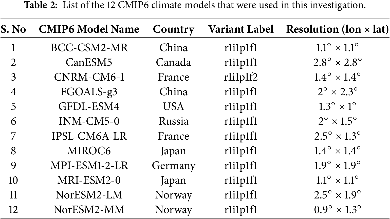
As shown in Table 2, this study evaluates 12 CMIP6 climate model simulations to assess their ability to replicate temperature and precipitation in the research area. Climate model data were obtained from the Earth System Grid Federation (ESGF) portal (https://esgf-node.llnl.gov/search/cmip6/) for both the historical period (1984–2014) and the future period (2015–2100). This study considers two forcing scenarios: SSP2-4.5 and SSP5-8.5, representing different Shared Socioeconomic Pathways (SSPs). The selection of GCMs was based on the following criteria: (i) availability of projections for the three primary climatic variables rainfall, maximum temperature, and minimum temperature; (ii) inclusion of future projections under SSP2-4.5 and SSP5-8.5 (CMIP6); (iii) completion of the first realization ensemble (r1i1p1f1) for historical runs across all models; and (iv) demonstrated performance in previous studies over East Africa and/or parts of Ethiopia [35–38]. The CMIP6 models used in this study have native horizontal resolutions of approximately 110–280 km, which limits their ability to explicitly represent localized convective extremes and orographic rainfall over the steep elevation range of the OGRB (235–3625 m). MIP6 model outputs with differing native resolutions were harmonized to a common 0.5° × 0.5° grid using bilinear interpolation implemented in Climate Data Operators (CDO) [39]. Bilinear interpolation is widely recommended for continuous variables such as temperature and precipitation because it preserves large-scale spatial gradients and avoids artificial discontinuities while maintaining the geographic integrity of the original fields [40]. The re-gridding was performed after bias correction at native resolution to minimize smoothing of extremes and to ensure that statistical adjustments were not affected by spatial transformation [41]. Spatial consistency was evaluated by comparing interpolated fields with independent station observations, confirming that elevation-controlled gradients and seasonal patterns were retained without detectable spatial displacement. Additional sensitivity tests using nearest-neighbour and conservative remapping showed differences of less than 3% in basin-averaged indices, indicating that the selected approach does not introduce significant artificial variability at the scale of the Omo–Gibe Basin [6]. Acknowledging this limitation, we note that higher-resolution statistical or dynamical downscaling would be expected to better capture sub-grid variability and topography-driven precipitation processes, and this represents an important direction for future work. To assess methodological sensitivity, a supplementary nearest-neighbour interpolation test was performed for a subset of stations, which showed negligible influence on seasonal mean fields but greater spread in extreme-index values, indicating that fine-scale application of the interpolated fields should be interpreted with caution. The interpolated outputs were also compared against station climatology to confirm consistency at the aggregated scale of analysis. The data extracted for each station from the CMIP6 model NetCDF files was converted to Microsoft Excel format using RStudio and organized for analysis.

2.3 Methods

Model Performance Analysis

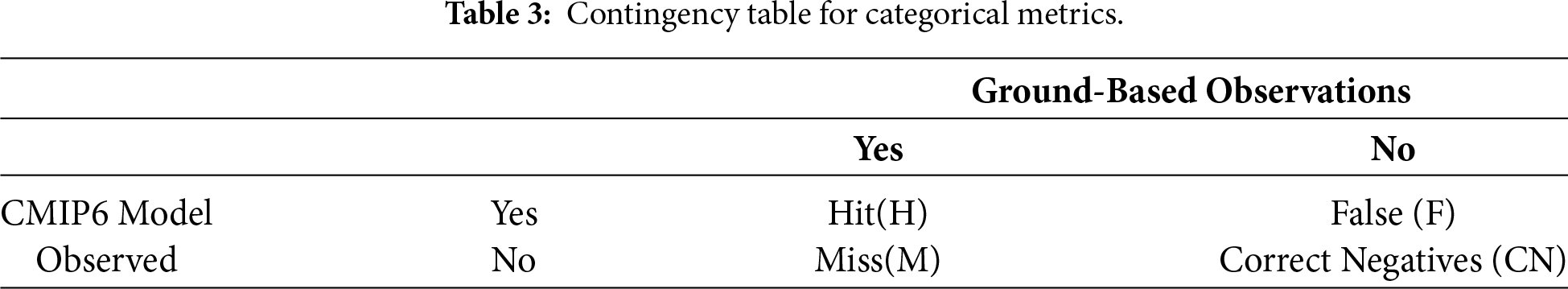
The performance of CMIP6 models was quantitatively assessed using both continuous statistical measures and categorical evaluation metrics. A commonly used contingency table is the 2 × 2 table, which categorizes events as follows: hits (H), where both simulation and observations detect an event; misses (M), where the simulation detects an event but observations do not; false alarms (F), where the simulation predicts an event that is not observed; and true nulls, where neither detects an event. This contingency table is used to define the following metrics [42]. The overall study framework and spatial context of the analysis are illustrated in Fig. 2.

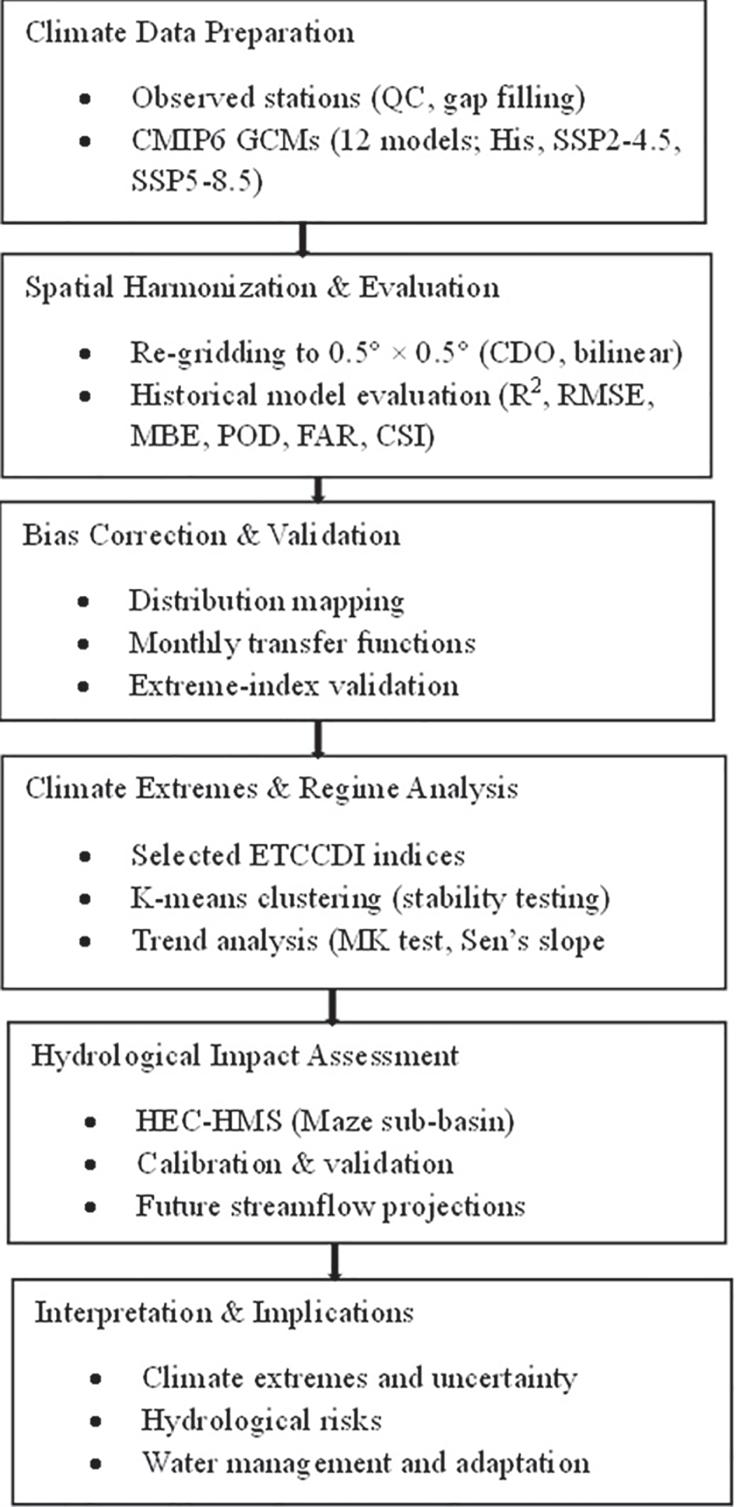
Figure 2: Methodological framework for CMIP6-based climate extremes and hydrological impact assessment over the Omo–Gibe River Basin.

2.3.1 Validation of CMIP6 Climate Models Statistically

The performance of individual CMIP6 models and the ensemble was evaluated annually by comparing simulated precipitation and temperature with observations. The ensemble mean used in this study represents the average of all CMIP6 datasets. Annual means were derived from monthly data, and CMIP6 simulations were further evaluated through statistical analysis and validation against observational records. The performance metrics used in this study were statistically significant and included the mean bias error (MBE), root mean square error (RMSE), and coefficient of determination (R2). The MBE assesses how well the mean of the CMIP6 model matches the mean of the observed data. A bias ratio closer to 0 indicates that the CMIP6 model’s precipitation and temperature estimates are closer to the observed values, suggesting better accuracy. The RMSE quantifies the distance between the estimated CMIP6 and observed data, with a value of 0 representing a perfect fit. The R2 measures the strength of the relationship between the CMIP6 models and observed data, with a value near 0 indicating no relationship and a value near 1 indicating a strong relationship. The parameters are defined in Eqs. (1)–(3):

R2=∑i=1N(Oi−O¯)(pi−p¯)∑iN(Oi−O¯)2∑iN(pi−p¯)2(1)

MBE=1N∑i=1N(pi−Oi)(2)

RMSE=∑iN(Pi′−Oi)2N(3)

where N, Oi, pi, O¯, and p¯ represent the number of observations, the observed values, the predicted values, the mean of the observed values, and the mean of the predicted values, respectively.

2.3.2 Categorical Validation Indices

In the categorical evaluation of extreme events, the terms “observed” and “modelled” are used to clearly distinguish station-based observations from CMIP6 historical model outputs. An extreme event is defined as a day exceeding the station-specific 95th percentile threshold. The hit-and-miss analysis was conducted exclusively for the historical period to evaluate how well CMIP6 models reproduce observed extreme events at the daily timescale. A “hit” occurs when both observed and modelled data indicate an extreme event on the same day, a “miss” when an observed extreme is not captured by the model, and a “false alarm” when the model indicates an extreme event that is not observed. These classifications are aggregated over the historical period to compute the probability of detection (POD), false alarm ratio (FAR), and critical success index (CSI). Extreme-event detection was evaluated using contingency metrics (POD, FAR and CSI) (Table 3), with events defined relative to the station-specific 95th-percentile threshold. The POD represents the fraction of reference observations correctly detected by the simulation, with values ranging from 0 (no ability) to 1 (perfect detection). The FAR refers to the fraction of events detected by the simulation but not confirmed by the reference observations, with 0 indicating a perfect score. The CSI combines POD and FAR to reflect the overall performance of the simulation relative to reference observations. CSI values range from 0 (no skill) to 1 (perfect ability). For each station and CMIP6 model, the total numbers of hits (H), misses (M), and false alarms (F) were accumulated across all days in the historical period. These aggregated counts were then used to compute standard categorical performance metrics. The following formulas were used to calculate the POD, FAR, and CSI values:

POD=HH+M(4)

FAR=FH+F(5)

CSI=HH+M+F(6)

where H, M, and F represent the number of hits, misses, and false alarms, respectively.

2.3.3 Bias Correction

Given the inherent biases in raw GCM outputs, it is essential to apply bias correction before performing impact assessment analyses [43,44]. After selecting the representative CMIP6 models for the OGRB, observed data were used to downscale the models from coarser to finer spatial resolutions. The CMhyd software was employed in this study for bias correction of simulated climate data from RCMs and GCMs [45]. The CMhyd software provides eight bias correction methods, including linear scaling (multiplicative), delta change correction (multiplicative), precipitation local intensity scaling, power transformation of precipitation, and distribution mapping for both precipitation and temperature bias correction. Additionally, linear scaling (additive), delta change correction (additive), and variance scaling are used for temperature bias correction. In this study, the distribution-mapping bias-correction method was selected after sensitivity testing against quantile mapping and variance scaling, as it produced lower residual bias in the upper-tail percentiles (90th–99th) and better reproduced the empirical distribution of extreme indices such as R95pTOT, Rx1day, TNn and TXn, whereas quantile mapping introduced instability in sparsely sampled extremes and variance scaling did not adequately correct distributional bias and also this approach was selected based on its documented advantages in previous research and its suitability for adjusting the selected CMIP6 models with observed data. To preserve temporal and spatial dependence, the transformation was applied as a monotonic correction to the full daily time series, thereby retaining the original sequencing of wet and dry spells and maintaining inter-site covariance across the basin. Although transfer functions were estimated at the monthly scale to account for seasonal variability in bias, they were applied to daily values so that sub-monthly extremes remained embedded in the corrected records. Post-correction validation was performed not only for mean climatology but also explicitly for ETCCDI extreme indices, confirming improved representation of both the magnitude and temporal behavior of extremes relative to the raw model simulations. The distribution mapping methodology is widely used in climate change studies as an effective bias-correction strategy [46–49]. The main objective was to adapt the transfer function parameters of GCM-simulated data to match those of the observed data, using the monthly mean values as a basis. This bias correction technique aligns the observed distribution function with the distribution of the simulated GCM data [50]. Two transfer functions are used to describe climate data: a Gaussian distribution for temperature and a gamma distribution for precipitation. The cumulative probability of simulated temperature data is computed, and based on this probability, the corrected temperature value is determined. For precipitation, a random precipitation intensity is initially generated to calculate the cumulative probability of the simulated precipitation. This cumulative probability is then used to determine the bias-corrected precipitation value [50].

2.3.4 Clustering and Pattern Detection

Clustering is a classification technique that groups similar objects into a single cluster, while dissimilar objects are placed in separate clusters. Various clustering techniques for pattern recognition have been discussed in the literature [51,52]. The K-means clustering method, a widely used technique, was employed in this study to group temperature and precipitation time series across various time scales and to identify stations with similar rainfall patterns. The iterative K-means technique, introduced by MacQueen, produces consistent results regardless of the initial starting point [53]. A key challenge when using K-means clustering is determining the optimal number of clusters [51,52]. In this study, Silhouette analysis was used to address this issue. Introduced by Belgian statistician Peter Rousseeuw [54], the Silhouette value is a metric that measures an object’s cohesiveness (similarity to its cluster) relative to its separation from other clusters. The Silhouette value ranges from −1 to +1, with higher values indicating that the object is well-matched to its cluster and poorly matched to neighbouring clusters. The clustering design may result in too many or too few clusters if a significant portion of the points have low or negative silhouette values [55]. Cluster robustness was assessed through repeated random initializations, yielding stable spatial groupings. To address multiple testing across indices, clusters and scenarios, a Bonferroni-adjusted significance threshold was applied. The silhouette coefficient for a given data point, i, can be calculated using the formula below.

S(i)=b(i)−a(i)max{a(i),b(i)}(7)

where, S(i) is the silhouette coefficient of the data point i; a(i) is the average distance between i and all the other data points in the cluster to which i belongs; b(i) is the average distance from i to all clusters to which i does not belong.

2.3.5 Climate Extremes Indices

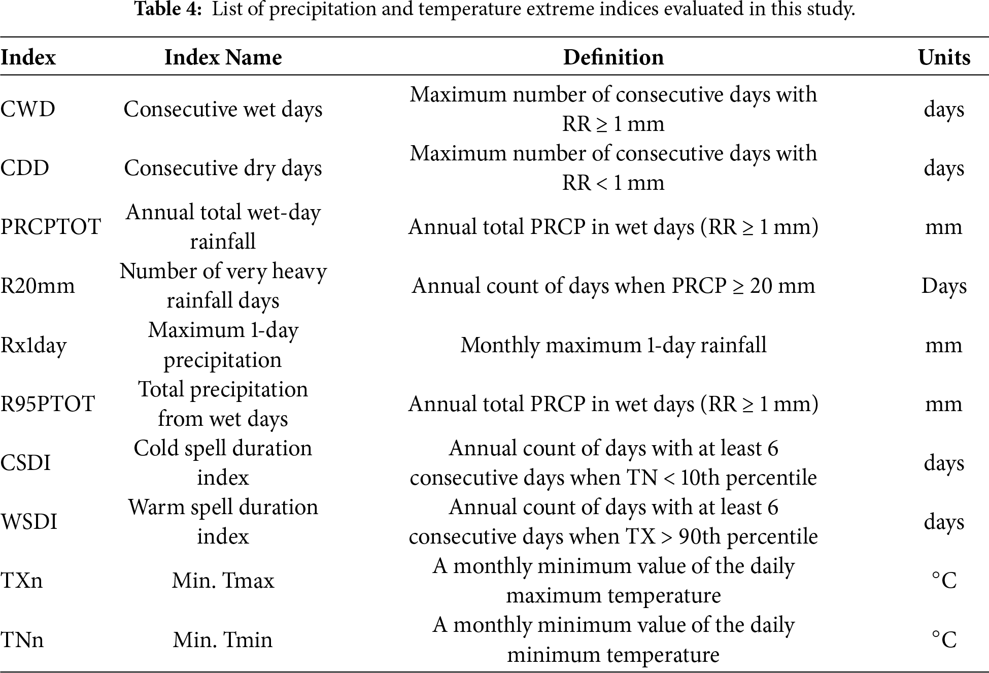
The Expert Team on Climate Change Detection and Indices (ETCCDI) [56] recommends 27 core precipitation and temperature indices. Detailed information and a complete list of these indices are available on the ETCCDI website: http://etccdi.pacificclimate.org/list_27_indices.shtml. This study focused on a select few of the most significant extreme temperature and precipitation indices. To enhance interpretability and policy relevance, the analysis focuses on a core set of ETCCDI indices that directly inform water-resource management and climate-risk assessment, including R95pTOT, Rx1day, CDD, TXx, and TNn. This prioritization enables clearer interpretation of key risks while maintaining comprehensive documentation of extreme climate behavior. The ETCCDI [56] provided six precipitation extreme indices and four temperature extreme indices used in this study. The precipitation indices are: Consecutive Wet Days (CWD), Consecutive Dry Days (CDD), Maximum 1-Day Precipitation (Rx1day), Total Precipitation from Wet Days (R95PTOT), Total Wet Day Precipitation Amount (PRCPTOT), and Very Heavy Rainfall (R20mm). The temperature indices include: Cold Spell Duration Index (CSDI), Warm Spell Duration Index (WSDI), Minimum Maximum Temperature (TXn), and Minimum Minimum Temperature (TNn). CWD, Rx1day, R95PTOT, and CDD are examples of extreme rainfall indices that are useful for managing water resources, agriculture, and determining flow storage and drainage. CDD also represents water shortages that affect crop growth and is used to assess drought and low-flow events. To evaluate water stress and evapotranspiration, CSDI and WSDI are employed. Table 4 provides detailed information on these extreme indices. For each observation station, as well as for all historical and projected data from the 12 CMIP6 GCMs across the OGRB, extreme precipitation and temperature indices are calculated using Climate Data Tools (CDT) version 7 and the R package climdex. pcic.

2.3.6 Test of Trend Analysis

For trend assessment in the hydro-meteorological dataset, the non-parametric Mann-Kendall (MK) trend test, recommended by the World Meteorological Organization [57], was used in this study. The trend’s significance was evaluated at a 95% significance level. The MK test calculates an overall score for the datasets, which is then compared with a critical value to determine whether the trend in the meteorological data is increasing, decreasing, or insignificant. The first step is to identify the signs of the sample results. The function Sign (Xj − Xi) indicates values of −1, 0, or +1, based on the sign of (Xj − Xi), where j > i. The function is computed as follows:

S=∑i=1n−1∑j=i+1nsign(xj−Xi)(8)

Sign(Xj−Xi)={+1,if(Xj−Xi)>00,if(Xj−Xi)=0−1,if(Xj−Xi)<0(9)

where ‘X’ represents the observation value, ‘n’ is the number of observations in the time series, ‘S’ is the ranking score (Mann-Kendall sum), and ‘Xj’ and ‘Xi’ represent consecutive meteorological data points in the month, with i < j. The values of S are interpreted as follows: ‘+’ for an increasing trend, ‘−’ for a decreasing trend, and ‘0’ for no trend. When n exceeds 10, the Mann-Kendall statistic is used to calculate the standard normal Z test statistic:

Z={1−SVar(S),ifS>00,ifS=01+SVar(S),ifS<0(10)

The significance of the statistical trend was assessed using the Z value. According to [58], the non-parametric Mann-Kendall trend test was applied to determine if the trend was monotonically increasing or decreasing, while the non-parametric Sen’s slope method was used to calculate the slope of linear trends. Modified Mann-Kendall tests can also be employed to detect trends in data impacted by autocorrelation. To address the issue of serial correlation in trend analysis, [59] proposed a variance correction approach. After detrending the data, a substantial serial correlation coefficient is used to determine the effective sample size. The modified VAR(S) statistics can then be computed using the equation from [60]:

VAR(S)=(n(n−1)(2n+5)18)⋅(nn∗)(11)

where nn∗ indicates a correction brought on by the data’s autocorrelation. An expression is required to evaluate nn∗.

Here, the correction factor nn∗ It is adjusted to the autocorrelated data as:

nn∗=1+(2n3−3n2+2n)∑f=1n−1(n−f)(n−f−1)(n−f−2)pe(f)(12)

where n represents the real number of observations and ρe(f) refers to the autocorrelation function of the observation ranks.

ρe(f) Signifies the autocorrelation between ranks of observations and can be estimated as:

ρ(f)=2sin⁡(π6)ρe(f)(13)

2.3.7 Hydrological Engineering Center-Hydrological Modelling System (HEC-HMS) Model

This model was developed to address water balance equations in both continuous and event-based hydrologic modelling by simulating the hydrological processes of watershed systems [61]. It is widely used for simulating precipitation-runoff relationships across various geographic regions, incorporating key components such as base flow, direct runoff, river routing, reservoir operations, and other hydrologic losses (US Army Corps., 2021). HEC-HMS is a semi-distributed hydrologic model designed to simulate the hydrological processes of watershed systems. Its configuration consists of a basin model, a meteorological model, control parameters, and time-series input data [62]. Over time, it has been enhanced to address a wide range of applications, including flood hydrographs, runoff from small urban and natural watersheds, and large river basin water supply management [63]. The primary input variables for HEC-HMS include precipitation, minimum and maximum temperatures, observed flow, base flow, and various watershed characteristics obtained from multiple sources.

Hydrological simulations were conducted for the Maze sub-basin, and results are interpreted primarily within this spatial context. The Maze sub-basin was selected due to the availability of reliable discharge observations and its representativeness of key hydro-climatic and physiographic conditions in the upper Omo–Gibe system, including rainfall seasonality, elevation gradients, and dominant land-cover types. Nevertheless, hydrological responses may differ in downstream sub-basins with contrasting topography, regulation, or land use. Accordingly, basin-wide implications are discussed qualitatively, and quantitative conclusions are restricted to the Maze sub-basin.

2.3.8 Hydrological Model Calibration and Validation

Model calibration is a systematic process of adjusting parameter values to accurately represent hydrological processes until the model’s output aligns with observed data. Model validation, on the other hand, evaluates the model’s ability to reproduce observed data beyond the calibration period. In the Maze watershed, model calibration was performed over 10 years (1992–2001), followed by validation over 5 years (2002–2006) at the watershed outlet. Calibration can be done manually or automatically; in this study, both methods were applied to both models. Before calibration, a sensitivity analysis was conducted to determine the initial parameter values. The next step is manual calibration, where the most sensitive parameters are manually adjusted until the simulated and observed hydrographs achieve a satisfactory match. In automatic calibration, the model iteratively modifies parameters to optimize the chosen objective function. Finally, the bias-corrected data from two SSP scenarios (SSP2-4.5 and SSP5-8.5) are used to run the HEC-HMS model for future streamflow simulations.

The performance of the HEC-HMS model was assessed using statistical metrics to evaluate the accuracy and reliability of its predictions in comparison to observed data. During calibration and validation, simulated and observed hydrographs were visually inspected to assess the model’s ability to reproduce observed streamflow. Additionally, efficiency metrics such as relative volume error (RVE), percent bias (PBIAS), coefficient of determination (R2), and Nash-Sutcliffe efficiency (NSE) were used to evaluate model performance. NSE ranges from −∞ to 1, where a value of 1 indicates a perfect match. A model’s performance is generally considered satisfactory when NSE falls between 0.5 and 1. The coefficient of determination (R2) ranges from 0 to 1, with values closer to 1 indicating better model performance, while R2 values below 0.5 suggest poor performance. Bias is calculated as the ratio of the difference between simulated and observed values to the observed values. A bias lower than ±10% indicates a near-perfect model, between ±10% and ±15% represents a good model, while values exceeding ±25% indicate an unacceptable prediction [64]. The relative volume error (RVE) measures the average volume difference between observed and simulated streamflow and is calculated using the following formula:

NSE=1−∑i=1n(Qo,i−Qp,i)2∑i=1n(Qo,i−Qo,i¯)2(14)

R2=∑i=1N(Oi−O¯)(pi−p¯)∑iN(Oi−O¯)2∑iN(pi−p¯)2(15)

PBIAS=∑(Qo;i−Qp,i)∑Qo,i∗100(16)

RVE=1−∑i=1n(Qo,i−Qp,i)∑i=1nQo,i∗100(17)

where Qo,i is the observed streamflow is at time step i and Qp,i is the simulated streamflow at time step i. The variable n represents the number of observations. The overbar (O¯ and p¯) denotes the mean values of the observed and simulated streamflow, respectively. Similarly, Oi and pi represent the observed and simulated values at each time step.

3  Results and Discussion

3.1 Cluster Analysis

Although the silhouette scores are relatively low, this reflects the presence of gradual spatial gradients and overlapping climatic influences across the basin rather than the absence of meaningful structure. Clustering was therefore applied as an exploratory tool to group areas with broadly similar extreme-climate behavior, rather than to define sharply separated regimes. Sensitivity analyses using alternative clustering methods (hierarchical clustering and k-medoids) and multiple random initializations yielded comparable spatial patterns and trend directions, supporting the robustness of the identified groupings. These results indicate that the clustering framework provides a useful means of summarizing spatial variability, while recognizing its inherent limitations in regions characterized by continuous climatic transitions. According to the silhouette coefficient, the optimal number of clusters for precipitation and mean monthly temperature is three and two, respectively, corresponding to the highest silhouette scores of 0.255 and 0.015 [32]. Table 1 and Fig. 1 display the clusters produced by the k-means algorithm using average monthly precipitation and temperature data from 21 OGRB stations. A comprehensive description of the climate characteristics of the three clusters in the Omo-Gibe Basin can be found in the previously published study [32]. The climatic characteristics of the three clusters within the OGRB exhibit notable spatial and seasonal variability, as shown in Fig. 3. Cluster 1 experiences the highest rainfall, following a unimodal pattern with a pronounced peak in June–July, reaching over 250 mm, indicating a relatively wet climate. Cluster 2 also shows a unimodal rainfall pattern, peaking around July, but with lower totals (approximately 200 mm) compared to Cluster 1. In contrast, Cluster 3 demonstrates a distinct bimodal rainfall distribution, with peaks in May and September and a noticeable dry spell during June and July, suggesting a transition to semi-arid or sub-humid conditions. Temperature patterns further differentiate the clusters: Cluster 1 exhibits higher maximum temperatures (Tmax) ranging from about 27°C to 30°C, while minimum temperatures (Tmin) remain relatively stable between 15°C and 17°C. Cluster 2 shows slightly lower Tmax values (26°C to 29°C) and cooler Tmin values (around 12°C to 15°C), especially during the rainy season. The observed differences reflect the influence of topography, elevation, and regional climate drivers across the basin.

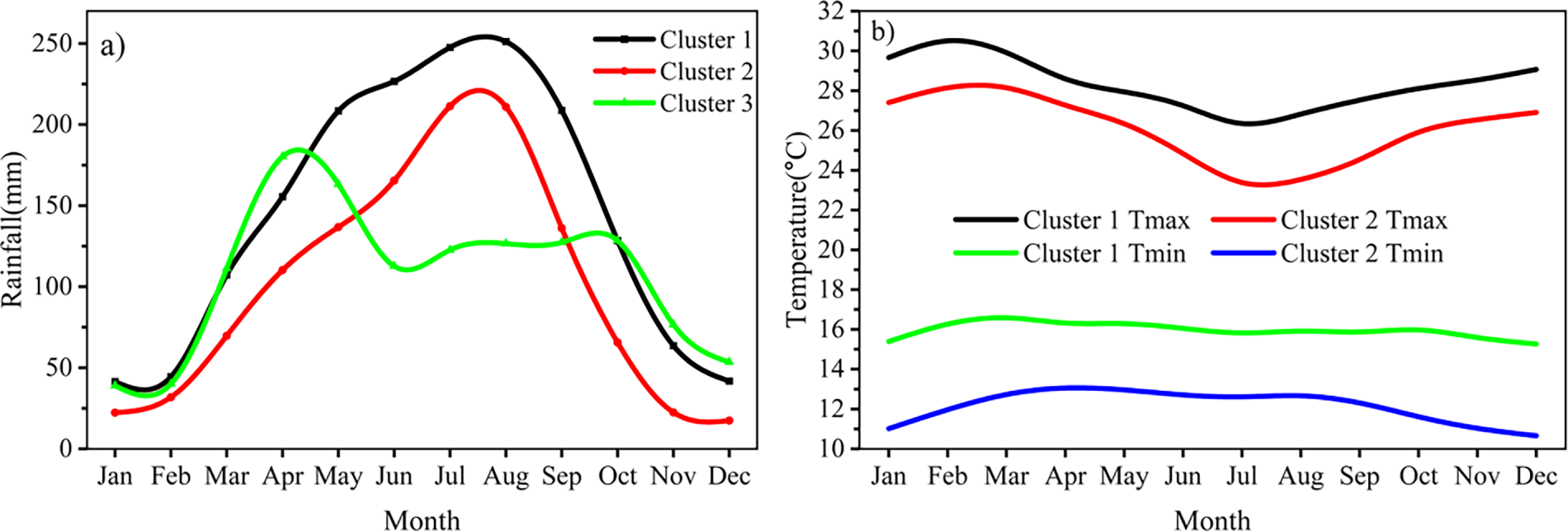
Figure 3: Mean monthly rainfall (a), maximum and minimum temperature (b) for Cluster 1, Cluster 2, and Cluster 3 of the Omo Gibe basin.

Fig. 4 illustrates the distribution of rainfall for the three identified clusters and maximum (Tmax) and minimum (Tmin) temperatures for the different clusters. The box plot shows clear differences in rainfall characteristics among the three clusters (Fig. 4a). Cluster 1 experiences the highest rainfall overall, with a relatively high median and a wide interquartile range, indicating substantial variability in rainfall amounts. The long whiskers suggest the occurrence of both very low and extremely high rainfall events, implying that this cluster is prone to intense and fluctuating rainfall conditions. Cluster 2 has the lowest median rainfall and the widest overall range, extending to very low values, which reflects highly irregular rainfall patterns. This cluster likely represents areas with inconsistent or seasonal rainfall, where dry periods are common but can occasionally be interrupted by heavy rainfall events. In contrast, Cluster 3 exhibits moderate rainfall levels, with a median slightly higher than that of Cluster 2 and a narrower interquartile range. This indicates more consistent and stable rainfall, with fewer extreme values compared to the other clusters. Overall, Cluster 1 is the wettest and most variable, Cluster 2 is the driest and most erratic, and Cluster 3 represents regions with moderate and relatively predictable rainfall patterns.

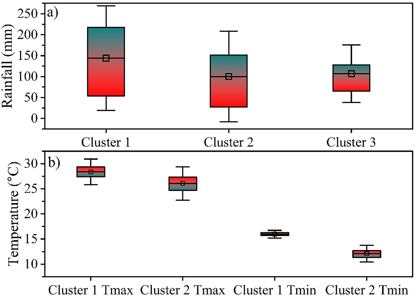
Figure 4: Box plot of rainfall distribution across clusters (a) and Box plot of maximum and minimum temperature across clusters (b).

The box plot illustrates clear differences in both maximum and minimum temperatures between the two clusters (Fig. 4b). For maximum temperature (Tmax), Cluster 1 shows higher values overall, with a higher median and upper range, indicating generally warmer daytime conditions and greater variability in maximum temperatures. In contrast, Cluster 2 has a lower median Tmax and a slightly narrower spread, suggesting comparatively cooler and more consistent maximum temperatures. Regarding minimum temperature (Tmin), Cluster 1 again records higher values, with a median around the mid-teens, reflecting warmer nighttime conditions and limited variability. Cluster 2 exhibits notably lower minimum temperatures, with a lower median and a wider spread, indicating cooler nights and greater fluctuations in Tmin. Overall, Cluster 1 is characterized by consistently warmer conditions both during the day and at night, while Cluster 2 experiences cooler temperatures, particularly at night, with slightly higher variability in minimum temperatures.

3.2 Evaluation of Model Performance

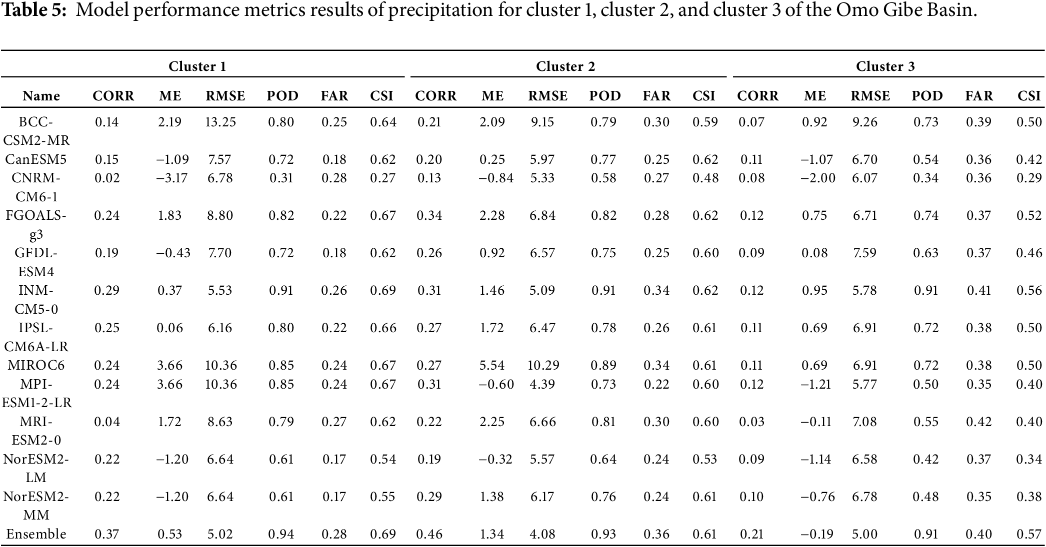
The 12 CMIP6 models were evaluated for their ability to reproduce precipitation and temperature over Clusters 1, 2, and 3 in the OGRB using performance metrics described in the Methods section, including R2, MBE, RMSE, POD, FAR, and CSI. Models with strong performance are characterized by high R2, POD, and CSI values, accompanied by low MBE, RMSE, and FAR values, whereas poorly performing models exhibit the opposite behaviour. Table 5 summarizes the accuracy of the ensemble mean and the 12 individual CMIP6 models in reproducing observed precipitation in Clusters 1, 2, and 3 of the OGRB. In the southern region (Cluster 3), the best-performing models are INM-CM5-0 (0.12, 0.947, 5.779, 0.906, 0.409, 0.556) and FGOALS-g3 (0.188, 0.75, 0.705, 0.741, 0.367, 0.518). For the western region (Cluster 1), the models with the highest skill are INM-CM5-0 (0.294, 0.368, 5.525, 0.913, 0.258, 0.693) and IPSL-CM6A-LR (0.253, 0.061, 6.159, 0.802, 0.215, 0.658), as shown in Table 4. In contrast, the CNRM-CM6-1 and MRI-ESM2-0 models show relatively weak performance for observed precipitation in Clusters 1 and 3. In the northern region (Cluster 2), the top-performing models are INM-CM5-0 (0.305, 1.46, 5.086, 0.913, 0.336, 0.624) and MPI-ESM1-2-LR (0.308, 0.596, 4.388, 0.728, 0.219, 0.604). By comparison, the MIROC6 model performs poorly relative to the other CMIP6 models. The values in parentheses represent R2, MBE, RMSE, POD, FAR, and CSI, respectively.

Although some models showed relatively weaker skill, we retained the full ensemble to preserve structural uncertainty and avoid exclusion-based bias, consistent with recommendations in recent CMIP6 evaluation studies, such as [65]. Equal weighting was therefore adopted to represent the full range of plausible climate responses; however, we acknowledge that performance-based model weighting may further refine projections, and we identify this as a useful direction for future work. In addition to statistical evaluation, we assessed the capacity of the models to represent key regional processes relevant to the OGRB, including monsoon-driven moisture transport, orographic precipitation enhancement over the basin’s complex topography, and large-scale circulation features. This process-based assessment complements the quantitative metrics and provides a physically grounded interpretation of model skill across the basin.

3.3 Future Precipitation and Temperature Extreme Indices Trends

The heat map illustrates projected Z-score changes in climate indices for each cluster over two future periods, 2023–2053 (near term) and 2054–2084 (far term), under the SSP2-4.5 and SSP5-8.5 scenarios, with non-significant changes indicated by dots and statistically significant trends at the 95% confidence level (p < 0.05) (Fig. 5), while the full numerical results are provided in the Supplementary Materials. Overall, both the magnitude and statistical significance of projected changes increase from the near-term to the far-term period and from the moderate-emission (SSP2-4.5) to the high-emission (SSP5-8.5) scenario, as reflected by stronger colour intensity and greater spatial coherence.

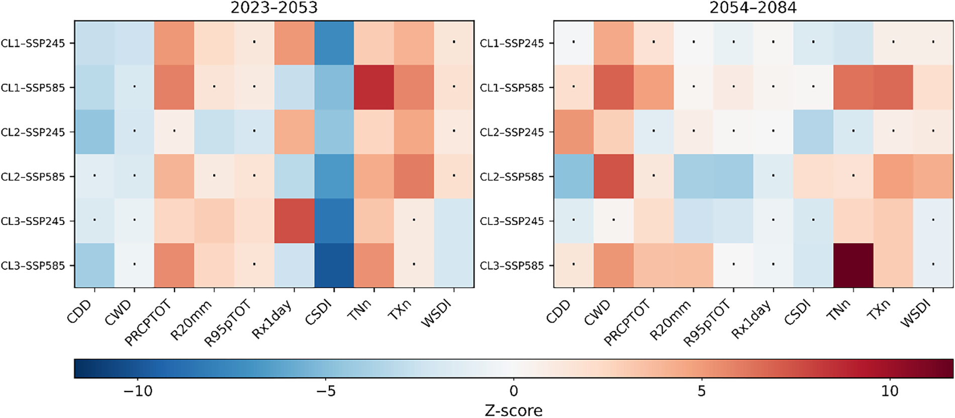
Figure 5: Projected Z-score changes in climate indices for 2023–2053 (left) and 2054–2084 (right) under SSP245 and SSP585 for each cluster. Dots (·) indicate non-significant changes (p ≥ 0.05). The color scale is symmetric for both periods. CL1, CL2, and CL3 represent Cluster 1, Cluster 2, and Cluster 3, respectively.

Cluster 1 exhibits relatively weak to moderate Z-score changes in the near-term period under SSP2-4.5, with several indices showing non-significant trends, indicating limited short-term deviation from historical variability. Under SSP5-8.5, positive and negative anomalies become more pronounced, particularly for temperature-related and extreme precipitation indices, although some remain statistically insignificant. In the far-term period, trends intensify markedly under both scenarios. Several indices shift toward stronger positive Z-scores under SSP2-4.5, indicating increased warming and wetter extremes, while under SSP5-8.5, these signals are amplified, with fewer non-significant indices and robust, statistically significant shifts toward more extreme climatic conditions.

Trend analysis confirms these patterns. Most precipitation and temperature extreme indices in Cluster 1 show statistically significant trends in the near term under SSP2-4.5, except for R95pTOT and WSDI, which exhibit positive but non-significant trends. PRCPTOT increases significantly by 6.37 mm yr−1 (SSP2-4.5) and 8.73 mm yr−1 (SSP5-8.5). CWD shows a significant increasing trend under both scenarios, while CDD increases significantly under SSP5-8.5. TNn increases significantly under SSP5-8.5 but decreases under SSP2-4.5. WSDI shows a significant increasing trend under SSP5-8.5.

Cluster 2 shows more heterogeneous behaviour. In the near-term period under SSP2-4.5, most indices exhibit weak anomalies with many non-significant trends. Under SSP5-8.5, clearer warming signals emerge, particularly for temperature extremes, while precipitation indices show mixed responses. In the far-term period, contrasts between scenarios become more pronounced: SSP2-4.5 produces moderate warming signals with weaker rainfall responses, whereas SSP5-8.5 yields stronger and more coherent Z-score patterns.

Trend results indicate a significant increase in PRCPTOT under SSP5-8.5 (5.32 mm yr−1), while no significant trend is detected under SSP2-4.5. R20mm shows a significant decreasing trend under SSP5-8.5. CWD increases significantly under both scenarios, whereas CDD decreases significantly. R95pTOT decreases significantly under SSP5-8.5. WSDI increases significantly under SSP5-8.5, while TNn and TXn do not exhibit significant trends under either scenario.

Cluster 3 is characterized by subdued near-term changes under SSP2-4.5, with many indices near zero and several non-significant trends, suggesting short-term climatic stability. Under SSP5-8.5, slight positive shifts emerge for temperature indices, though significance remains limited in the near term. In the far-term period, clearer and more systematic responses develop: SSP2-4.5 produces gradual but consistent changes, while SSP5-8.5 results in stronger, statistically significant anomalies across most indices.

PRCPTOT increases significantly in Cluster 3 under both scenarios, by 7.49 mm yr−1 (SSP2-4.5) and 8.42 mm yr−1 (SSP5-8.5). R20mm increases significantly under SSP5-8.5 but decreases under SSP2-4.5. CWD increases significantly under SSP5-8.5, while no significant trend is observed under SSP2-4.5. CDD shows no significant trend under either scenario. TNn and TXn exhibit significant warming trends under both scenarios, with Sen’s slopes of approximately 0.02°C–0.05°C yr−1. CSDI shows a significant decreasing trend under SSP5-8.5, indicating fewer cold spells.

R95pTOT does not show statistically significant trends in Cluster 1 under either scenario and decreases significantly in Cluster 2 under SSP5-8.5. In contrast, Cluster 3 exhibits a stronger increase in R95pTOT, particularly under SSP5-8.5, although significance varies by scenario. This spatial amplification is interpreted as the combined effect of thermodynamic and dynamic processes. Projected warming enhances atmospheric moisture availability in line with Clausius–Clapeyron scaling, while monsoon-related low-level moisture transport and orographic uplift along the Rift escarpment strengthen moisture convergence and convective development. The consistency of this pattern across CMIP6 models, its agreement with historical heavy-rainfall gradients, and its alignment with known moisture-transport pathways suggest that the enhanced R95pTOT response in Cluster 3 reflects robust physical mechanisms rather than modelling artifacts. The maximum 1-day precipitation (Rx1day) does not exhibit statistically significant trends in any cluster, although positive and negative Z-scores indicate weak upward or downward tendencies under SSP5-8.5 and SSP2-4.5, respectively.

Overall, all clusters experience greater and more statistically significant projected changes in the far-future period than in the near future, with SSP5-8.5 consistently producing larger Z-score magnitudes than SSP2-4.5. Cluster 1 shows the most pronounced and robust intensification of warming and wet extremes, Cluster 2 displays mixed but strengthening trends with high sensitivity to index type, and Cluster 3 transitions from near-term stability to clear long-term climate change signals, particularly under the high-emission scenario.

In addition to the ensemble-mean projections, we also quantify the spread and robustness of the CMIP6 ensemble. For each extreme index, inter-model variability is reported using both the standard deviation and inter-quartile range, and model-agreement maps are used to distinguish areas where at least 75% of models agree on the direction of change (robust signal) from regions with weak consensus. Probability distributions of selected indices are also presented to illustrate the full spread of projected outcomes rather than relying on single-value estimates.

3.4 Results of the Calibration and Validation of the HEC-HMS Model

The performance of the HEC-HMS model in simulating streamflow for the Maze sub-basin was evaluated through calibration (1992–2001) and validation (2002–2006). The results are summarized in Table 6, and the daily hydrograph is illustrated in Fig. 6, where the calibration and validation periods are shown on the left and right sides of the green vertical line, respectively. The model’s effectiveness was evaluated using the Nash-Sutcliffe Efficiency (NSE), Coefficient of Determination (R2), Relative Volume Error (RVE), and Percent Bias (PBIAS) metrics.

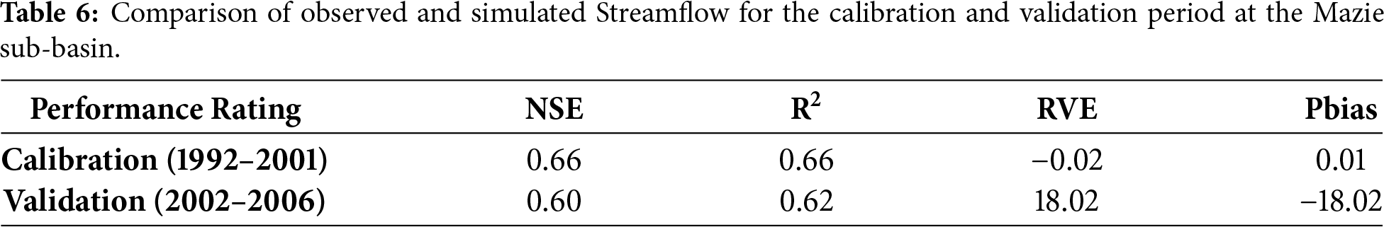
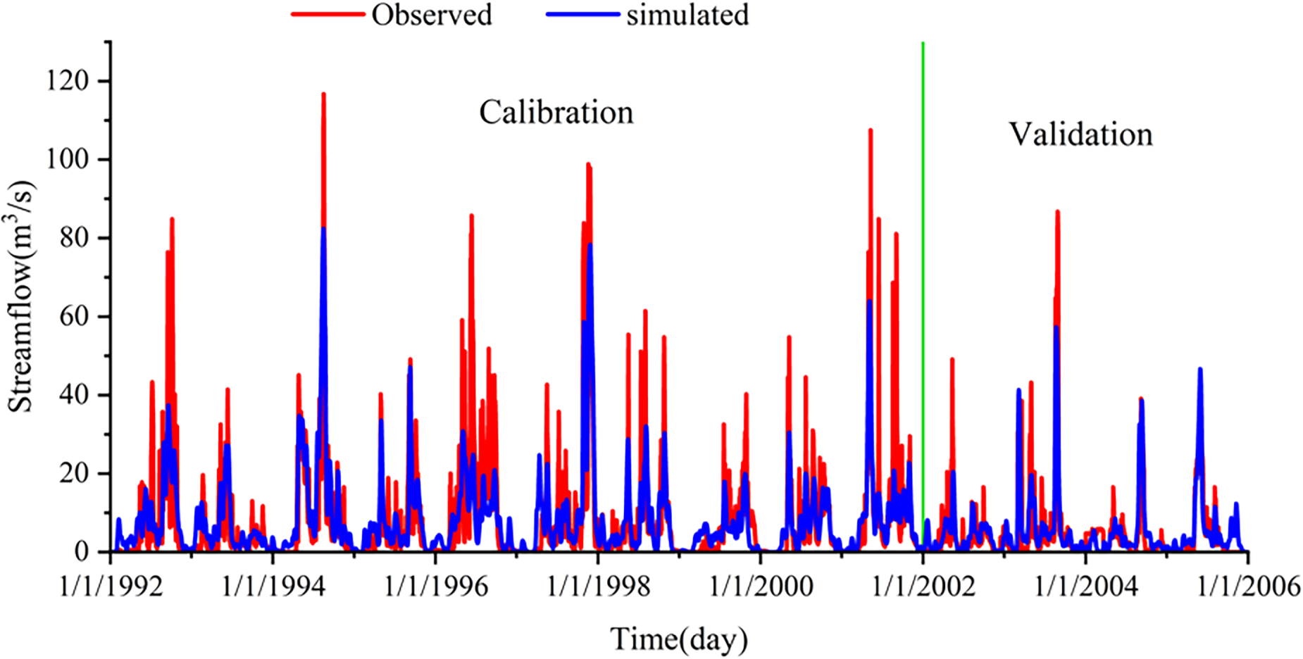
Figure 6: Daily streamflow graph of calibration and validation for the Maze sub-basin, left and right, respectively, from the vertical green line.

The calibration and validation results of the HEC-HMS model for the Maze sub-basin demonstrate satisfactory performance in simulating streamflow. With NSE values of 0.66 and 0.60 for calibration (1992–2001) and validation (2002–2006), respectively, the model effectively captures streamflow variability, though with slightly reduced performance during validation. R2 values of 0.66 and 0.62 indicate a moderate to strong correlation between the observed and simulated streamflow, suggesting that the model captures the overall flow patterns reasonably well. While RVE (−0.02) and PBIAS (0.01%) suggest minimal bias in calibration, validation results show an 18% underestimation of streamflow, likely due to uncertainties in input data, model parameterization, or hydrological variability. The −18.02% validation bias indicates a systematic underestimation of streamflow, which is likely related to structural limitations in the representation of groundwater storage and baseflow recession, leading to reduced simulated discharge during high-flow periods. Seasonal inspection shows that the bias is more pronounced during peak-flow months, suggesting greater sensitivity to runoff generation and routing processes than to low-flow dynamics. This behaviour has important implications for non-stationary climate projections, as parameter sets calibrated under historical conditions may not fully capture hydrological responses under altered climate regimes. We also recognize that model performance is partly dependent on the selected calibration period and that alternative calibration windows or model structures could produce different outcomes. Accordingly, we interpret projected streamflow changes with caution and recommend future work employing multi-model hydrological frameworks to better characterize structural uncertainty and its interaction with GCM uncertainty. The daily hydrograph (Fig. 6) confirms that the model replicates streamflow patterns well, though peak flows are under-predicted. Despite these limitations, the model remains a reliable tool for future streamflow simulations in the OGRB, particularly for climate change impact assessments and water resource management planning.

3.5 Impacts of Climate Change on Streamflow in the Future Periods

3.5.1 Impacts on Future Mean Monthly Flow

This study aimed to evaluate projected streamflow under SSP2-4.5 and SSP5-8.5 scenarios for three future periods (2023–2039, 2040–2056, and 2057–2073) relative to the reference period (1992–2006). To simulate streamflow, bias-corrected temperature, precipitation, and estimated evapotranspiration time series for the selected future periods were used as input. Fig. 7a illustrates that during the base period, the highest hydrograph typically occurs between May and August. However, under future climate change scenarios, the hydrograph pattern is projected to shift, showing two distinct peaks, one in May to June and another in October, contrasting with the single peak observed in the reference period. This shift indicates potential alterations in seasonal runoff patterns, which may have significant implications for water resource management and flood risk assessment in the region.

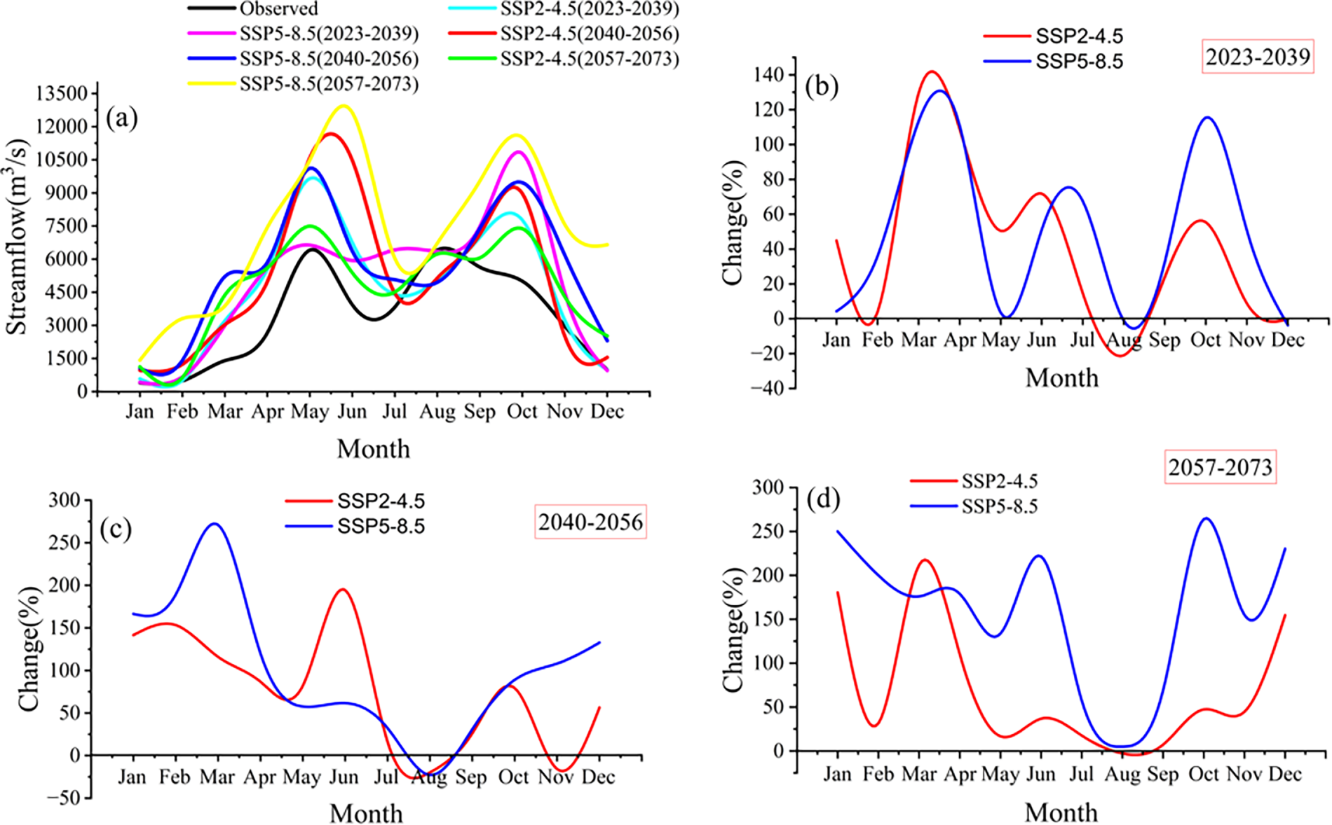
Figure 7: Projected monthly mean streamflow: (a) 2023–2039, 2040–2056, 2057-2073 and percentage change: (b) 2023–2039; (c) 2040–2056, and (d) 2057-2073 under SSP2-4.5 and SSP5-8.5, compared to the baseline period 1992–2006.

Projected monthly streamflow in August is anticipated to decline more sharply than in any other month under both SSP2-4.5 and SSP5-8.5 scenarios across all three future periods. In the period from 2023 to 2039, the predicted streamflow is also anticipated to slightly decrease in December under both scenarios (Fig. 7b). Additionally, for the period 2040–2056, a decrease in streamflow is expected in November under SSP2-4.5 (Fig. 7c). In contrast, streamflow in January, March, and October is projected to increase the most under the SSP5-8.5 scenario, while reductions are expected in August under both SSP2-4.5 and SSP5-8.5 scenarios. The increase in streamflow under the SSP5-8.5 scenario is more pronounced compared to SSP2-4.5. Notably, months such as March and October could experience substantial increases in streamflow, raising the potential risk of flooding. Conversely, the significant decrease in streamflow during specific months, such as August, may lead to water shortages in the region.

The projected transition from a unimodal to a bimodal runoff regime is interpreted as arising from a combination of extended late-season rainfall and delayed subsurface and baseflow response, which together contribute to the emergence of a secondary October flow peak. The timing shift is quantified using a centre-of-timing metric, which indicates a forward displacement of this additional peak relative to the historical hydrograph. Inter-model agreement shows that the bimodal signal is reproduced by most CMIP6 models, although the magnitude of the secondary peak varies among ensemble members, indicating a partially robust but model-dependent transition. From an operational perspective, the emergence of dual peaks has potential implications for Gibe reservoir storage regulation, release scheduling and flood-buffer allocation, and may increase the likelihood of late-season flood events compared with the historical unimodal regime.

Table 7 summarizes the mean monthly, seasonal, and annual percentage change in streamflow for the periods 2023–2039, 2040–2056, and 2057–2073, in comparison to the reference period 1992–2006. It is projected that both monthly and annual streamflow will increase over the future periods. Specifically, for the 2023–2039 period, monthly streamflow is expected to increase by 40.9% under the SSP2-4.5 scenario and 48.4% under the SSP5-8.5 scenario. The annual streamflow is projected to rise by 36.3% and 46.3% for SSP2-4.5 and SSP5-8.5, respectively.

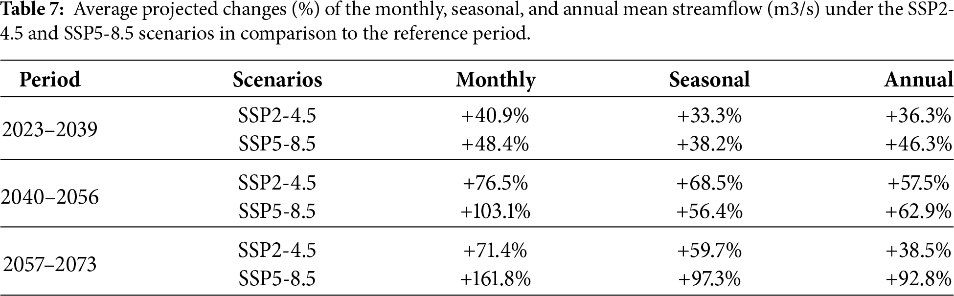
For the 2040–2056 period, monthly streamflow is projected to increase by 76.5% and 103.1% under SSP2-4.5 and SSP5-8.5, respectively, while annual streamflow is expected to rise by 57.5% and 62.9%. Similarly, for the 2057–2073 period, the projected increase in monthly streamflow is 71.4% under SSP2-4.5 and 161.8% under SSP5-8.5, while annual streamflow is expected to rise by 38.5% and 92.8%, respectively, under the two scenarios. Overall, the mean projected changes in streamflow vary across monthly, seasonal, and annual scales. Monthly streamflow changes are generally more pronounced than the annual changes. Additionally, streamflow increases are expected to be greater under the SSP5-8.5 scenario compared to SSP2-4.5.

3.5.2 Impacts on Seasonal and Annual Flow

Seasonal analysis in this study was conducted using baseline data, dividing the year into four seasons: winter (December, January, February), spring (March, April, May), summer (June, July, August), and autumn (September, October, November). The projected mean seasonal and annual streamflow for the periods 2023–2039, 2040–2056, and 2057–2073 under the SSP2-4.5 and SSP5-8.5 scenarios are presented in Fig. 8. The mean seasonal streamflow is projected to increase across all seasons in each of the three future periods under both scenarios, primarily due to the anticipated increase in precipitation.

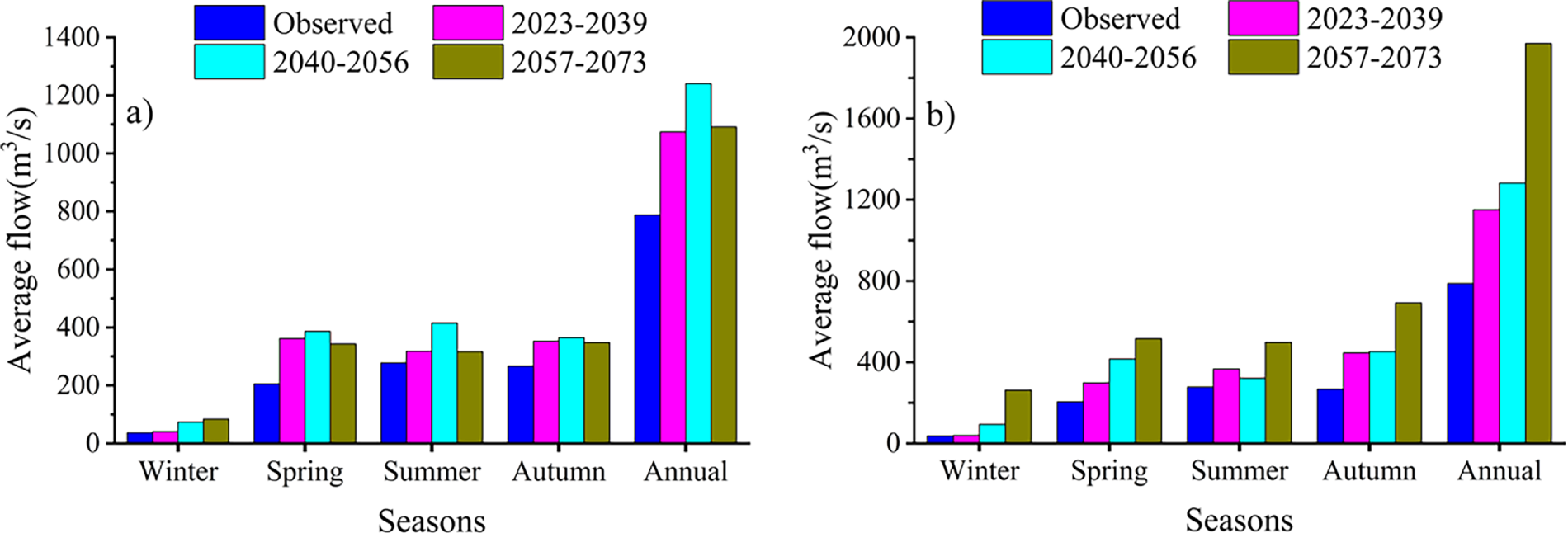
Figure 8: Projected average seasonal and annual streamflow: (a) SSP2-4.5 and (b) SSP5-8.5, for the three future periods 2023–2039, 2040–2056, 2057–2073, compared to the baseline period 1992–2006.

Fig. 9 illustrates the mean seasonal and annual changes in streamflow for the upcoming periods under both SSP2-4.5 and SSP5-8.5 scenarios. The anticipated changes in streamflow for winter, spring, summer, autumn, and annual periods, relative to the reference period, were calculated. The results indicate that streamflow is projected to increase across all seasons as well as on an annual basis under both SSP2-4.5 and SSP5-8.5 scenarios. Notably, under the SSP5-8.5 scenario, the rate of change in streamflow is projected to accelerate during the 2057–2073 period compared to the other future periods (Fig. 9b). On average, the increases in streamflow for winter, spring, summer, and autumn are projected to be 79.5%, 76.8%, 25.9%, and 33.0%, respectively, under SSP2-4.5, and 69.7%, 65.2%, 42.3%, and 78.8% under SSP5-8.5. In all scenarios (monthly, seasonal, and annual), streamflow is likely to increase.

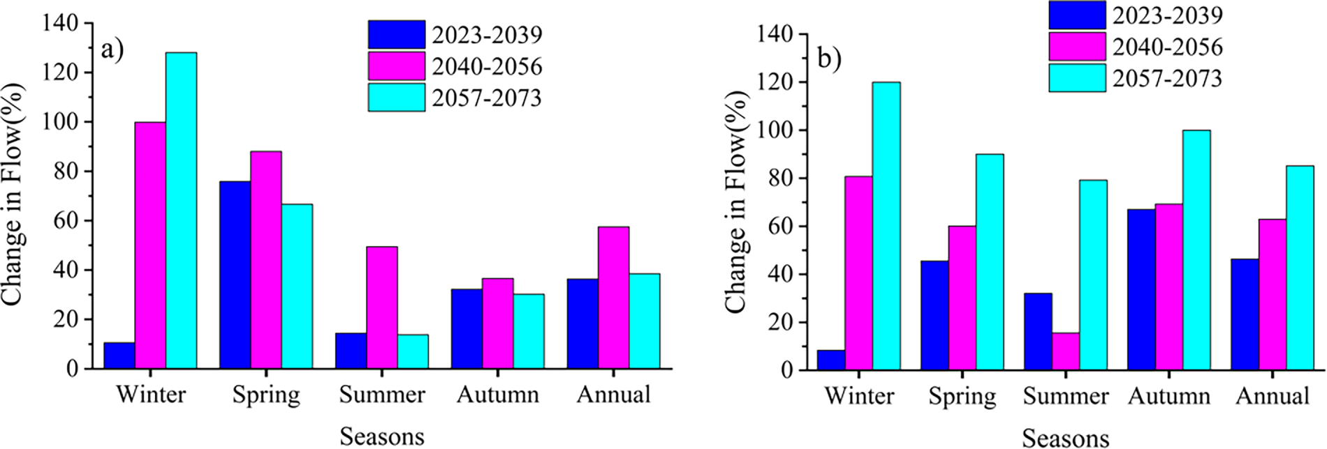
Figure 9: Seasonal and annual changes in stream flow: (a) SSP2-4.5 and (b) SSP5-8.5, for the three future periods 2023–2039, 2040–2056, and 2057–2073.

4  Discussion

This study evaluated the performance of 12 CMIP6 models over the OGRB by comparing them against observed daily precipitation and temperature data, along with extreme climate indices, for the period 1985–2014. Bias correction significantly improved the model simulations, particularly through distribution mapping, which reduced systematic errors and enhanced the correlation with observed values. Continuous and categorical evaluation metrics such as RMSE, R2, POD, FAR, and CSI were used to assess model performance. Models like INM-CM5-0, FGOALS-g3, and IPSL-CM6A-LR showed the best precipitation simulation in certain clusters, while INM-CM5-0, BCC-CSM2-MR, and MPI-ESM1-2-LR were found to simulate temperature extremes more effectively. These findings are consistent with previous research showing CMIP6 models generally outperform their CMIP5 counterparts in simulating East African climate characteristics [66,67].

Analysis of extreme climate indices such as CDD, CWD, R95pTOT, R20mm, PRCPTOT, TXn, TNn, WSDI, and CSDI revealed spatially heterogeneous trends across the basin. For example, increasing trends in PRCPTOT and R20mm in several clusters suggest a rise in total precipitation and heavy rainfall events, while CDD exhibited a decreasing pattern in many areas, indicating a possible reduction in dry spells. These results support the notion that climate extremes are intensifying in Ethiopia, with increased rainfall variability and frequency of extreme events [1,68]. Under the SSP2-4.5 and SSP5-8.5 scenarios, near-term (2023–2053) and mid-term (2054–2084) projections further emphasize a continuation of these trends, with more pronounced changes under the high-emission SSP5-8.5 pathway [32].

Hydrologically, the use of bias-corrected climate data as input into the HEC-HMS model for the Maze sub-basin revealed significant changes in the basin’s streamflow regime. Unlike the historical single peak (May–August), future projections show a shift toward a bimodal hydrograph with peaks in May–June and October. This hydrological response is likely driven by changes in rainfall timing and intensity, with annual streamflow projected to increase by 54.7% (SSP2-4.5) and 92.7% (SSP5-8.5) in the mid-term. Such increases could exacerbate flood risks while posing challenges for water resource planning. These findings align with previous hydrological modelling studies in Ethiopia that projected increased streamflow due to enhanced precipitation under climate change scenarios [69–71]. The projected increases in future streamflow are relatively large and should be interpreted in light of both physical plausibility and uncertainty. Intensification of heavy precipitation indices, increased atmospheric moisture associated with warming, and shifts in rainfall timing provide a physically consistent basis for higher runoff generation; however, the magnitude of projected changes varies substantially across models and scenarios. Additional uncertainty arises from bias-correction procedures and hydrological model structure, particularly in representing runoff generation and baseflow processes under non-stationary climate conditions. Consequently, projected increases are best interpreted as indicating heightened potential for elevated flows rather than precise quantitative forecasts. From a management perspective, these results suggest increased flood risk and greater pressure on reservoir operation and flood-buffer capacity, underscoring the need for adaptive, uncertainty-aware water-resources planning rather than reliance on single deterministic projections.

Compared to other major Ethiopian basins, the OGRB exhibits both similarities and differences in climate trends. For instance, studies in the Awash River Basin have reported increasing heavy rainfall events and warming trends that are consistent with those observed in the OGRB [72]. However, the rainfall regime in the OGRB is more complex due to its topographic and climatic variability, with both unimodal and bimodal rainfall patterns present in different clusters, unlike the predominantly unimodal pattern in the Awash. Similarly, the Blue Nile Basin has experienced rising temperatures and more frequent warm nights, with projections showing significant increases in runoff [73,74]. In contrast, the OGRB exhibits more pronounced shifts in seasonal streamflow peaks, highlighting regional variability in climate responses and underscoring the need for basin-specific adaptation planning. Rather than reiterating numerical results, the Discussion emphasizes interpretation of the projected changes in a broader regional context. The magnitude and direction of projected increases in temperature and heavy precipitation are broadly consistent with findings from other Ethiopian and East African basins, including the Blue Nile, Baro–Akobo, and Awash systems, which similarly report intensified extremes under warming scenarios. From an adaptation perspective, these changes imply increased pressure on flood management, reservoir operation, and irrigation planning, particularly in basins with expanding infrastructure and land-use change. The results underscore the importance of flexible, scenario-aware water management strategies that explicitly account for uncertainty and evolving climate risks, thereby supporting climate-resilient policy and investment decisions.

Projected trend magnitudes are interpreted within an explicit uncertainty framework and compared against established regional and global benchmarks. Sen’s slope estimates are presented alongside inter-model spread and confidence intervals, and their magnitudes are evaluated relative to IPCC AR6 assessments, which report robust warming trends over East Africa of approximately 0.2°C–0.4°C per decade under intermediate to high emission scenarios, alongside increased intensity of heavy precipitation events but with substantial uncertainty in mean rainfall trends [75]. In this context, statistically significant but small Sen’s slope values are interpreted cautiously, particularly where uncertainty ranges overlap across models or scenarios, indicating limited practical significance despite formal significance. Emphasis is therefore placed on trends that are both statistically robust and consistent with broader regional signals reported in recent IPCC and CMIP6-based assessments.

Furthermore, temperature extremes in the OGRB showed statistically significant upward trends in TXn and TNn, confirming a warming signal in minimum and maximum temperature indices. This is in agreement with the national and regional assessments that found increasing trends in nighttime temperatures and heat extremes [75,76]. The warm spell duration index (WSDI) and cold spell duration index (CSDI) provide further insight into thermal extremes, where future projections suggest longer warm periods and shorter cold periods. These trends are critical for sectors like agriculture and public health, where prolonged heat exposure could impact crop productivity and increase heat-related illnesses.

The implications of these findings for water resource management are profound. The dual-peak streamflow pattern projected for the future, alongside increasing rainfall intensities, necessitates a re-evaluation of existing hydrological infrastructure and flood control strategies. Experiences from other basins, like the Awash and Baro-Akobo, indicate that traditional floodplain infrastructure may be inadequate under intensified hydrological regimes [77]. Adaptive water management, including the development of multi-reservoir systems, improved early warning mechanisms, and climate-smart agricultural practices, will be crucial in mitigating these impacts. Claims of more pronounced hydroclimatic shifts are supported by statistically significant trend estimates, with larger Sen’s slope magnitudes and narrower interquartile ranges observed under high-emission scenarios, indicating both stronger signals and increased model agreement. However, the present analysis is limited to climate extremes and streamflow responses and does not explicitly account for associated impacts on water quality, sediment transport, or ecological flow regimes. Changes in extreme rainfall and altered flow timing may substantially affect sediment loads, reservoir siltation, and downstream aquatic ecosystems, which are not represented within the current modeling framework. These aspects should be addressed in future integrated assessments to avoid overinterpretation of flow-based results alone.

This study has several limitations that should be considered when interpreting the results. First, the hydrological responses assessed here reflect climate forcing only and do not incorporate future land-use or land-cover change; although the basin already contains approximately 29.82% intensively farmed land, further agricultural expansion, deforestation, soil compaction, or irrigation development could independently modify runoff generation, evapotranspiration, and infiltration capacity, potentially amplifying or dampening the simulated climate-driven changes. Relatedly, the hydrological modelling relied on historical land-use data, and future land-cover dynamics under alternative socioeconomic pathways were not explored. Second, while the use of gridded observational datasets and bias correction is effective, it may still underrepresent micro-climatic variability, particularly in areas with sparse meteorological stations. Third, groundwater–surface-water interactions are represented in a simplified manner in HEC-HMS, which may limit the model’s ability to capture baseflow contributions and subsurface storage dynamics, especially during dry-season flow recession. Fourth, human water-management activities—such as existing and planned hydropower reservoirs (including prospective Gibe IV–V), irrigation abstractions, and potential inter-basin transfers were not explicitly modelled and could substantially modify future discharge regimes relative to the naturalized simulations presented here. Fifth, although our extreme-climate analysis primarily focused on 95th-percentile indices, very rare extremes (e.g., 99th–99.9th percentiles) remain more uncertain and may not be fully captured by the available data record and model ensemble. Finally, hydrological model structural uncertainty was not explored; different model formulations or parameterizations may yield different runoff sensitivities, and the use of high-resolution regional climate models, multi-model hydrological ensembles, and formal uncertainty analyses would provide a more comprehensive and robust characterization of climate-impact uncertainty. These limitations emphasize that our projections should be interpreted as basin-scale climate impacts rather than precise predictions for fully managed catchments.

The HEC-HMS simulations are designed to assess basin-scale streamflow responses to projected changes in climate forcing and primarily represent changes in seasonal and mean flow characteristics rather than event-scale flood extremes. Extreme precipitation indices such as R95pTOT and Rx1day indicate increased rainfall intensity and frequency, which may contribute to higher peak flows and enhanced runoff generation; however, these indices are not directly translated into simulated flood magnitudes within the current modelling framework. Accordingly, projected streamflow changes are interpreted as indicative of altered flow regimes and potential shifts in high-flow conditions, rather than explicit flood-risk projections.

In summary, this study demonstrates that CMIP6 models, when bias-corrected, can provide reliable projections for both climate extremes and hydrological responses in the OGRB. The results also confirm that climate change will intensify both precipitation and temperature extremes, with direct implications for streamflow dynamics. Comparisons with other basins in Ethiopia reveal both consistent patterns of change and important spatial heterogeneities. These findings underscore the need for localized, climate-informed water management and adaptation planning to build resilience in the face of future climate uncertainty.

5  Conclusions

This study systematically evaluated the ability of twelve CMIP6 models to reproduce observed temperature and precipitation extremes over the Omo–Gibe River Basin and assessed future changes in key ETCCDI indices and associated hydrological responses under SSP2–4.5 and SSP5–8.5 scenarios. The model evaluation demonstrates that INM-CM5-0 and MPI-ESM1-2-LR show relatively higher skill in representing historical extremes, and that bias correction substantially improves model performance, providing a more reliable basis for future projections. Results indicate robust intensification of precipitation extremes, with significant increases in PRCPTOT (approximately +7.49 mm yr−1) and R95pTOT (approximately +8.42 mm yr−1), alongside a reduction in consecutive dry days, suggesting a shift toward wetter conditions. Concurrent warming trends in TXn and TNn (up to 0.05°C yr−1) imply increasing heat stress and heightened hydroclimatic variability. Hydrological simulations for the Maze sub-basin project show substantial increases in streamflow (up to ~92.8% by the 2070s) and shifts in seasonal flow timing, indicating elevated potential for high-flow conditions and flood risk. From a management perspective, these findings highlight the need for adaptive reservoir operation, enhanced flood preparedness, and climate-resilient water-resources planning that explicitly accounts for uncertainty. While the results provide decision-relevant insights, future work should incorporate high-resolution regional downscaling, alternative hydrological model structures, and explicit representation of land-use change and water regulation to further refine localized risk assessments and support long-term adaptation strategies in the basin.

Acknowledgement: The observed climate data used in this study were obtained from the Ethiopian Meteorology Institute (EMI). The CMIP6 GCM data were freely accessed from the Earth System Grid Federation (ESGF) website. The authors gratefully acknowledge these institutions for providing the data.

Funding Statement: The authors received no specific funding for this study.

Author Contributions: Fetene Muluken Chanie: conceptualization; writing—original draft; methodology; visualization; software; formal analysis; investigation; data curation; project administration. Mulugeta Genanu Kebede: writing—review and editing; validation; visualization; supervision; resources; conceptualization; methodology. Yared Godine Demeke: software; writing—review and editing; visualization; supervision; resources; conceptualization; methodology. Zelalem Bedaso: software; writing—review and editing; visualization; supervision; resources; conceptualization; methodology. All authors reviewed and approved the final version of the manuscript.

Availability of Data and Materials: Since the observed rainfall and temperature data obtained from the Ethiopian Meteorology Institute (EMI) and stream flow data from the Ministry of Water and Energy are available for self-use only, the authors do not have permission to share the data. However, the CMIP6 GCMs can be accessed on their website (https://esgf-node.llnl.gov/search/cmip6).

Ethics Approval: Not applicable.

Conflicts of Interest: The authors declare no conflicts of interest.

Supplementary Materials: The supplementary material is available online at https://www.techscience.com/doi/10.32604/rig.2026.076765/s1.

References

1. Gedefaw M. Assessment of changes in climate extremes of temperature over Ethiopia. Cogent Eng. 2023;10(1):2178117. doi:10.1080/23311916.2023.2178117. [Google Scholar] [CrossRef]

2. Stocker T. Climate change 2013: The physical science basis: Working group I contribution to the fifth assessment report of the intergovernmental panel on climate change. Cambridge, UK: Cambridge University Press; 2014. [Google Scholar]

3. Amato R, Steptoe H, Buonomo E, Jones R. High-resolution history: downscaling China’s climate from the 20CRv2c reanalysis. J Appl Meteor Climatol. 2019;58(10):2141–57. doi:10.1175/jamc-d-19-0083.1. [Google Scholar] [CrossRef]

4. Bekele D, Alamirew T, Kebede A, Zeleke G, Melese AM. Analysis of rainfall trend and variability for agricultural water management in Awash River Basin, Ethiopia. J Water Clim Change. 2017;8(1):127–41. doi:10.2166/wcc.2016.044. [Google Scholar] [CrossRef]

5. Misiani HO, Finney DL, Segele ZT, Marsham JH, Tadege A, Artan G, et al. Circulation patterns associated with current and future rainfall over Ethiopia and south Sudan from a convection-permitting model. Atmosphere. 2020;11(12):1352. doi:10.3390/atmos11121352. [Google Scholar] [CrossRef]

6. Ongoma V, Chen H, Gao C, Nyongesa AM, Polong F. Future changes in climate extremes over Equatorial East Africa based on CMIP5 multimodel ensemble. Nat Hazards. 2018;90(2):901–20. doi:10.1007/s11069-017-3079-9. [Google Scholar] [CrossRef]

7. Endris HS, Omondi P, Jain S, Lennard C, Hewitson B, Chang’a L, et al. Assessment of the performance of CORDEX regional climate models in simulating east African rainfall. J Clim. 2013;26(21):8453–75. doi:10.1175/jcli-d-12-00708.1. [Google Scholar] [CrossRef]

8. Ge F, Zhu S, Luo H, Zhi X, Wang H. Future changes in precipitation extremes over Southeast Asia: insights from CMIP6 multi-model ensemble. Environ Res Lett. 2021;16(2):024013. doi:10.1088/1748-9326/abd7ad. [Google Scholar] [CrossRef]

9. Kim YH, Min SK, Zhang X, Sillmann J, Sandstad M. Evaluation of the CMIP6 multi-model ensemble for climate extreme indices. Weather Clim Extrem. 2020;29:100269. doi:10.1016/j.wace.2020.100269. [Google Scholar] [CrossRef]

10. Klutse NAB, Quagraine KA, Nkrumah F, Quagraine KT, Berkoh-Oforiwaa R, Dzrobi JF, et al. The climatic analysis of summer monsoon extreme precipitation events over west Africa in CMIP6 simulations. Earth Syst Environ. 2021;5(1):25–41. doi:10.1007/s41748-021-00203-y. [Google Scholar] [CrossRef]

11. Srivastava A, Grotjahn R, Ullrich PA. Evaluation of historical CMIP6 model simulations of extreme precipitation over contiguous US regions. Weather Clim Extrem. 2020;29:100268. doi:10.1016/j.wace.2020.100268. [Google Scholar] [CrossRef]

12. Wehner M, Gleckler P, Lee J. Characterization of long period return values of extreme daily temperature and precipitation in the CMIP6 models: part 1, model evaluation. Weather Clim Extrem. 2020;30:100283. doi:10.1016/j.wace.2020.100283. [Google Scholar] [CrossRef]

13. Chen CA, Hsu HH, Liang HC. Evaluation and comparison of CMIP6 and CMIP5 model performance in simulating the seasonal extreme precipitation in the Western North Pacific and East Asia. Weather Clim Extrem. 2021;31(1):100303. doi:10.1016/j.wace.2021.100303. [Google Scholar] [CrossRef]

14. Sillmann J, Kharin VV, Zwiers FW, Zhang X, Bronaugh D. Climate extremes indices in the CMIP5 multimodel ensemble: part 2. Future climate projections. J Geophys Res Atmos. 2013;118(6):2473–93. doi:10.1002/jgrd.50188. [Google Scholar] [CrossRef]

15. Jiang Z, Li W, Xu J, Li L. Extreme precipitation indices over China in CMIP5 models. Part I: model evaluation. J Clim. 2015;28(21):8603–19. doi:10.1175/jcli-d-15-0099.1. [Google Scholar] [CrossRef]

16. Ayugi B, Jiang Z, Zhu H, Ngoma H, Babaousmail H, Karim R, et al. Comparison of CMIP6 and CMIP5 models in simulating mean and extreme precipitation over East Africa. Int J Climatol. 2021;41(15):6474–96. doi:10.1002/joc.7207. [Google Scholar] [CrossRef]

17. Eyring V, Bony S, Meehl GA, Senior CA, Stevens B, Stouffer RJ, et al. Overview of the coupled model intercomparison project phase 6 (CMIP6) experimental design and organization. Geosci Model Dev. 2016;9(5):1937–58. doi:10.5194/gmd-9-1937-2016. [Google Scholar] [CrossRef]

18. Marotzke J, Jakob C, Bony S, Dirmeyer PA, O’Gorman PA, Hawkins E, et al. Climate research must sharpen its view. Nat Clim Chang. 2017;7(2):89–91. doi:10.1038/nclimate3206. [Google Scholar] [PubMed] [CrossRef]

19. Koutroulis AG, Grillakis MG, Tsanis IK, Papadimitriou L. Evaluation of precipitation and temperature simulation performance of the CMIP3 and CMIP5 historical experiments. Clim Dyn. 2016;47(5):1881–98. doi:10.1007/s00382-015-2938-x. [Google Scholar] [CrossRef]

20. Nguyen P, Thorstensen A, Sorooshian S, Zhu Q, Tran H, Ashouri H, et al. Evaluation of CMIP5 model precipitation using PERSIANN-CDR. J Hydrometeorol. 2017;18(9):2313–30. doi:10.1175/jhm-d-16-0201.1. [Google Scholar] [CrossRef]

21. Li L, Li W, Ballard T, Sun G, Jeuland M. CMIP5 model simulations of Ethiopian Kiremt-season precipitation: current climate and future changes. Clim Dyn. 2016;46(9):2883–95. doi:10.1007/s00382-015-2737-4. [Google Scholar] [CrossRef]

22. Pietrangeli A, Pallavicini I. Hydroelectric cascade plants in the Omo Basin in Ethiopia. In: ICOLD 75th Annual Meeting; 2007 Jun 24–29; Saint Petersburg, Russia. p. 1–10. [Google Scholar]

23. Gebrechorkos SH, Taye MT, Birhanu B, Solomon D, Demissie T. Future changes in climate and hydroclimate extremes in east Africa. Earth’s Future. 2023;11(2):e2022EF003011. doi:10.1029/2022EF003011. [Google Scholar] [CrossRef]

24. Berhanu D, Alamirew T, Bewket W, Tarkegn TG, Zeleke G, Haileslassie A, et al. Evaluation of CMIP6 models in simulating seasonal extreme precipitation over Ethiopia. Weather Clim Extrem. 2025;47:100752. doi:10.1016/j.wace.2025.100752. [Google Scholar] [CrossRef]

25. Dogiso D, Muluneh A, Ketema A. Spatiotemporal analysis of CMIP6-based climate extremes and their implications for sustainable watershed management in the Gidabo watershed, Ethiopia. Sci Rep. 2025;15(1):28104. doi:10.1038/s41598-025-02408-x. [Google Scholar] [PubMed] [CrossRef]

26. Wondimu SA, Kenea TT, Tafesse KE. Evaluating climate extremes and their association with floods in the Baro Akobo River basin using CMIP6 and hydrological modelling. Nat Hazards. 2025;121(12):14229–53. doi:10.1007/s11069-025-07349-2. [Google Scholar] [CrossRef]

27. Orkodjo TP, Kranjac-Berisavijevic G, Abagale FK. Impact of climate change on future precipitation amounts, seasonal distribution, and streamflow in the Omo-Gibe basin, Ethiopia. Heliyon. 2022;8(6):e09711. doi:10.1016/j.heliyon.2022.e09711. [Google Scholar] [PubMed] [CrossRef]

28. Woldemariam TT. Impact assessment of climate change and anthropogenic actions on streamflow characteristics, hydropower and environmental flow of Omo-Gibe River Basin in Ethiopia. New Delhi, India: Indian Institute of Technology Delhi; 2019. [Google Scholar]

29. Avery S. Hydrological impacts of ethiopia’s Omo Basin on Kenya’s Lake Turkana water levels & fisheries prepared for the African Development Bank, Tunis. Irvine, CA, USA: Water Resource Associates; 2010. [Google Scholar]

30. Degefu MA, Bewket W. Variability, trends, and teleconnections of stream flows with large-scale climate signals in the Omo-Ghibe River Basin, Ethiopia. Environ Monit Assess. 2017;189(4):142. doi:10.1007/s10661-017-5862-1. [Google Scholar] [PubMed] [CrossRef]

31. Yericho BM, Mulugeta BA. Challenges and opportunities for implementation of integrated water resource management in Omo-Gibe Basin, Ethiopia. J Ecol Nat Environ. 2019;11(7):84–97. doi:10.5897/jene2019.0747. [Google Scholar] [CrossRef]

32. Chanie FM, Kebede MG, Demeke YG, Bedaso ZK, Tegen AD, Bayable E. Evaluating CMIP6 model accuracy in predicting and clustering precipitation and temperature trends in the omo-gibe river basin, Ethiopia. Atmos Ocean. 2025;63(1):57–77. doi:10.1080/07055900.2025.2485087. [Google Scholar] [CrossRef]

33. Dinku T, Hailemariam K, Maidment R, Tarnavsky E, Connor S. Combined use of satellite estimates and rain gauge observations to generate high-quality historical rainfall time series over Ethiopia. Int J Climatol. 2014;34(7):2489–504. doi:10.1002/joc.3855. [Google Scholar] [CrossRef]

34. Esayas B, Simane B, Teferi E, Ongoma V, Tefera N. Trends in extreme climate events over three agroecological zones of Southern Ethiopia. Adv Meteor. 2018;2018:7354157. doi:10.1155/2018/7354157. [Google Scholar] [CrossRef]

35. Alaminie AA, Tilahun SA, Legesse SA, Zimale FA, Tarkegn GB, Jury MR. Evaluation of past and future climate trends under CMIP6 scenarios for the UBNB (abayEthiopia. Water. 2021;13(15):2110. doi:10.3390/w13152110. [Google Scholar] [CrossRef]

36. Ayugi B, Ngoma H, Babaousmail H, Karim R, Iyakaremye V, Lim Kam Sian KTC, et al. Evaluation and projection of mean surface temperature using CMIP6 models over East Africa. J Afr Earth Sci. 2021;181:104226. doi:10.1016/j.jafrearsci.2021.104226. [Google Scholar] [CrossRef]

37. Gebresellase SH, Wu Z, Xu H, Wada IM. Evaluation of CMIP6 climate models for climate change impact assessments in Upper Awash Basin, Ethiopia. 2022. doi:10.21203/rs.3.rs-1231424/v1. [Google Scholar] [CrossRef]

38. Almazroui M, Saeed F, Saeed S, Nazrul Islam M, Ismail M, Klutse NAB, et al. Projected change in temperature and precipitation over Africa from CMIP6. Earth Syst Environ. 2020;4(3):455–75. doi:10.1007/s41748-020-00161-x. [Google Scholar] [CrossRef]

39. Schulzweida U. CDO user guide (version 2.0.0); 2021 [cited 2025 Jan 1]. Available from: 10.5281/zenodo.3539275. [Google Scholar] [CrossRef]

40. Maraun D. Bias correction, quantile mapping, and downscaling: revisiting the inflation issue. J Clim. 2013;26(6):2137–43. doi:10.1175/jcli-d-12-00821.1. [Google Scholar] [CrossRef]

41. Gudmundsson L, Bremnes JB, Haugen JE, Engen-Skaugen T. Technical Note: downscaling RCM precipitation to the station scale using statistical transformations-a comparison of methods. Hydrol Earth Syst Sci. 2012;16(9):3383–90. doi:10.5194/hess-16-3383-2012. [Google Scholar] [CrossRef]

42. Levine RA, Wilks DS. Statistical methods in the atmospheric sciences. J Am Stat Assoc. 2000;95(449):344. doi:10.2307/2669579. [Google Scholar] [CrossRef]

43. Cannon AJ, Sobie SR, Murdock TQ. Bias correction of GCM precipitation by quantile mapping: how well do methods preserve changes in quantiles and extremes? J Clim. 2015;28(17):6938–59. doi:10.1175/jcli-d-14-00754.1. [Google Scholar] [CrossRef]

44. Cannon AJ. Multivariate quantile mapping bias correction: an N-dimensional probability density function transform for climate model simulations of multiple variables. Clim Dyn. 2018;50(1):31–49. doi:10.1007/s00382-017-3580-6. [Google Scholar] [CrossRef]

45. Rathjens H, Bieger K, Srinivasan R, Chaubey I, Arnold JG. CMhyd user manual documentation for preparing simulated climate change data for hydrologic impact studies. 2016. 16 p. [Google Scholar]

46. Berg P, Feldmann H, Panitz HJ. Bias correction of high resolution regional climate model data. J Hydrol. 2012;448:80–92. doi:10.1016/j.jhydrol.2012.04.026. [Google Scholar] [CrossRef]

47. Mbaye ML, Haensler A, Hagemann S, Gaye AT, Moseley C, Afouda A. Impact of statistical bias correction on the projected climate change signals of the regional climate model REMO over the Senegal River Basin. Int J Climatol. 2016;36(4):2035–49. doi:10.1002/joc.4478. [Google Scholar] [CrossRef]

48. Olsson T, Jakkila J, Veijalainen N, Backman L, Kaurola J, Vehviläinen B. Impacts of climate change on temperature, precipitation and hydrology in Finland—Studies using bias corrected Regional Climate Model data. Hydrol Earth Syst Sci. 2015;19(7):3217–38. doi:10.5194/hess-19-3217-2015. [Google Scholar] [CrossRef]

49. Tschöke GV, Kruk NS, de Queiroz PIB, Chou SC, de Sousa Junior WC. Comparison of two bias correction methods for precipitation simulated with a regional climate model. Theor Appl Climatol. 2017;127(3):841–52. doi:10.1007/s00704-015-1671-z. [Google Scholar] [CrossRef]

50. Teutschbein C, Seibert J. Bias correction of regional climate model simulations for hydrological climate-change impact studies: review and evaluation of different methods. J Hydrol. 2012;456:12–29. doi:10.1016/j.jhydrol.2012.05.052. [Google Scholar] [CrossRef]

51. Javadi S, Hashemy SM, Mohammadi K, Howard KWF, Neshat A. Classification of aquifer vulnerability using K-means cluster analysis. J Hydrol. 2017;549(1):27–37. doi:10.1016/j.jhydrol.2017.03.060. [Google Scholar] [CrossRef]

52. Pratima D, Nimmakanti N. Pattern recognition algorithms for cluster identification problem. Int J Comput Sci Inform. 2013:185–92. doi:10.47893/ijcsi.2013.1089. [Google Scholar] [CrossRef]

53. MacQueen J. Some methods for classification and analysis of multivariate observations. Proc Fifth Berkeley Symp Math Stat Probab. 1967;1(14):281–97. [Google Scholar]

54. Rousseeuw PJ. Silhouettes: a graphical aid to the interpretation and validation of cluster analysis. J Comput Appl Math. 1987;20:53–65. doi:10.1016/0377-0427(87)90125-7. [Google Scholar] [CrossRef]

55. Shutaywi M, Kachouie NN. Silhouette analysis for performance evaluation in machine learning with applications to clustering. Entropy. 2021;23(6):759. doi:10.3390/e23060759. [Google Scholar] [PubMed] [CrossRef]

56. Zhang X, Alexander L, Hegerl GC, Jones P, Tank AK, Peterson TC, et al. Indices for monitoring changes in extremes based on daily temperature and precipitation data. Wires Clim Change. 2011;2(6):851–70. doi:10.1002/wcc.147. [Google Scholar] [CrossRef]

57. WMO. Analyzing long time series of hydrological data with respectto climate variability. Geneva, Switzerland: WMO Secr.; 1988. [Google Scholar]

58. Gilbert RO. Statistical methods for environmental pollution monitoring. Hoboken, NJ, USA: John Wiley & Sons; 1987. doi:10.2307/2531935. [Google Scholar] [CrossRef]

59. Yue S, Wang C. The Mann-Kendall test modified by effective sample size to detect trend in serially correlated hydrological series. Water Resour Manag. 2004;18(3):201–18. doi:10.1023/B:WARM.0000043140.61082.60. [Google Scholar] [CrossRef]

60. Hamed KH, Ramachandra Rao A. A modified Mann-Kendall trend test for autocorrelated data. J Hydrol. 1998;204(1–4):182–96. doi:10.1016/S0022-1694(97)00125-X. [Google Scholar] [CrossRef]

61. Jhs B, Alt F, Ad L, Lc A. The influence of spatial discretization on HEC-HMS modelling: a case study. Int J Hydrol. 2019;3(5):442–9. doi:10.15406/ijh.2019.03.00209. [Google Scholar] [CrossRef]

62. Kamarudin MKA, Toriman ME, Rosli MH, Juahir H, Aziz NAA, Azid A, et al. Analysis of meander evolution studies on effect from land use and climate change at the upstream reach of the Pahang River, Malaysia. Mitig Adapt Strateg Glob Change. 2015;20(8):1319–34. doi:10.1007/s11027-014-9547-6. [Google Scholar] [CrossRef]

63. Oleyiblo JO, Li ZJ. Application of HEC-HMS for flood forecasting in Misai and Wan’an catchments in China. Water Sci Eng. 2010;3(1):14–22. doi:10.3882/j.issn.1674-2370.2010.01.002. [Google Scholar] [CrossRef]

64. Hou Y, Zhang X, Song J, Na J. Conduction between left superior pulmonary vein and left atria and atria fibrillation under cervical vagal trunk stimulation. Colomb Med. 2008;39(3):227–34. doi:10.25100/cm.v39i3.590. [Google Scholar] [CrossRef]

65. Ayodele AP, Precious EE, Brhane ES, Seun AI. CMIP6 multi-model evaluation of summer extreme precipitation over East Asia. Model Earth Syst Environ. 2022;8(4):4749–63. doi:10.1007/s40808-022-01433-3. [Google Scholar] [CrossRef]

66. Iturbide M, Gutiérrez JM, Alves LM, Bedia J, Cerezo-Mota R, Cimadevilla E, et al. An update of IPCC climate reference regions for subcontinental analysis of climate model data: definition and aggregated datasets. Earth Syst Sci Data. 2020;12(4):2959–70. doi:10.5194/essd-12-2959-2020. [Google Scholar] [CrossRef]

67. Tegegne G, Melesse AM, Alamirew T. Projected changes in extreme precipitation indices from CORDEX simulations over Ethiopia, East Africa. Atmos Res. 2021;247:105156. doi:10.1016/j.atmosres.2020.105156. [Google Scholar] [CrossRef]

68. Korecha D, Barnston AG. Predictability of June–September rainfall in Ethiopia. Mon Weather Rev. 2007;135(2):628–50. doi:10.1175/mwr3304.1. [Google Scholar] [CrossRef]

69. Dile YT, Berndtsson R, Setegn SG. Hydrological response to climate change for Gilgel Abay River, in the Lake Tana Basin-Upper Blue Nile Basin of Ethiopia. PLoS One. 2013;8(10):e79296. doi:10.1371/journal.pone.0079296. [Google Scholar] [PubMed] [CrossRef]

70. Emiru NC, Recha JW, Thompson JR, Belay A, Aynekulu E, Manyevere A, et al. Impact of climate change on the hydrology of the upper awash river basin, Ethiopia. Hydrology. 2022;9(1):3. doi:10.3390/hydrology9010003. [Google Scholar] [CrossRef]

71. Gragn T, Kebede A, Berhanu S. Evaluation of climate change impacts on the water resources of Awata River Watershed, Genale Dawa Basin: southern Ethiopia. Acad Res J Agri Sci Res. 2019;7(7):414–22. doi:10.14662/ARJASR2019.124. [Google Scholar] [CrossRef]

72. Tadese MT, Kumar L, Koech R, Zemadim B. Hydro-climatic variability: a characterisation and trend study of the Awash River Basin, Ethiopia. Hydrology. 2019;6(2):35. doi:10.3390/hydrology6020035. [Google Scholar] [CrossRef]

73. Chakilu GG, Sándor S, Zoltán T. The dynamics of hydrological extremes under the highest emission climate change scenario in the headwater catchments of the upper blue Nile Basin, Ethiopia. Water. 2023;15(2):358. doi:10.3390/w15020358. [Google Scholar] [CrossRef]

74. Teklay A, Dile YT, Asfaw DH, Bayabil HK, Sisay K, Ayalew A. Modeling the impact of climate change on hydrological responses in the Lake Tana Basin. Ethiopia Dyn Atmos Oceans. 2022;97:101278. doi:10.1016/j.dynatmoce.2021.101278. [Google Scholar] [CrossRef]

75. Legg S. IPCC, 2021: climate change 2021—The physical science basis. Interaction. 2021;49(4):44–5. [Google Scholar]

76. Gebrechorkos SH, Hülsmann S, Bernhofer C. Regional climate projections for impact assessment studies in East Africa. Environ Res Lett. 2019;14(4):044031. doi:10.1088/1748-9326/ab055a. [Google Scholar] [CrossRef]

77. Gebisa BT, Dibaba WT. Ensemble modeling of the hydrological impacts of climate change: a case study of the Baro River sub-basin, Ethiopia. Hydrol Res. 2024;55(11):1143–60. doi:10.2166/nh.2024.066. [Google Scholar] [CrossRef]