Application of Time Serial Model in Water Quality Predicting

1  Introduction

Water is an important resource for human survival, and the quality of it directly affects the development and utilization of water resources. Since water quality changes are closely related to climate environment, seasonal changes and human activities, changes in river water quality are characterized by gradual changes, nonlinearity, and uncertainty [1], and it is difficult to accurately predict water quality changes. However, water quality prediction is of great significance to the planning and management of water resources and the environment. According to the prediction results, the water pollution situation can be predicted in advance, so that water pollution incidents can be prevented in advance as well.

With the continuous development of the Internet of Things technology and the Internet, the digital economy is developing rapidly, and big data and related technologies are increasingly affecting our daily life. By analyzing the big data generated in production and life [2,3], we can make predictions about the future [4,5]. In recent years, some scholars have done related research on water quality prediction. Xu et al. proposed a surface water quality prediction model based on Graph Neural Network (GNN), which uses GNN to model the spatial complexity of surface water quality monitoring sites. Compared with the traditional method, the performance of this method is significantly improved [6]. Luo et al. used ARIMA and Support Vector Regression (SVR) combined model to predict water quality. After the data is preprocessed, the ARIMA model is used to linearly fit it, and then the SVR model is used to predict the residuals to compensate for the nonlinear changes. The results show that the combined model prediction accuracy is significantly improved [7]. Based on the ARIMA model, Wang et al. introduced the Holt-Winters seasonal model for optimization, and established a general water quality prediction model with eutrophication index TP and total nitrogen as parameters. Through self-calibration, the model can significantly reduce the cost of reservoir water quality prediction, improve the accuracy of water quality prediction, and provide a method for the study of dynamic changes in reservoir water quality parameters [8]. Huan et al. proposed a dissolved oxygen prediction model based on random forest (RF) and Long Short-Term Memory network (LSTM). This method firstly reduced the input dimensionality of the data. Then, the LSTM prediction model of river dissolved oxygen was constructed to fit the relationship between water quality data and dissolved oxygen, and finally the real water quality data in the river was used for verification. The experimental results show that the RF-LSTM model had good prediction performance and can provide a reference for river water quality management [9]. Zhang et al. used the gray model and the residual correction method based on extreme learning machine regression to predict the values of water quality parameters, and then designed a T-S fuzzy neural network model to predict the water quality changes of the three monitoring sections in the Taihu Lake Basin [10]. Xue et al. improved the gray neural network model, which combined the advantages of gray neural network and Markov, and improved the prediction accuracy [11]. However, the grey model has higher prediction accuracy only when the original data changes exponentially. For the case where the sequence changes do not change exponentially, the prediction results may be deviated [12]. A collection of observations arranged in chronological order is called a time series. The main feature of the time series model is to admit the dependencies and correlations among observations. It is a dynamic model and can be applied to dynamic forecasting [13]. The ARIMA model is one of the more widely used time series modeling methods. Yang Yingmei conducted ARIMA modeling on the CPI data in Beijing. The model fits the data well and prediction error is small [14]. In order to improve the medium-term prediction accuracy of network traffic time series, Tian et al. proposed a method of compensating the ARIMA model with a Gaussian process regression model to improve the medium-term prediction accuracy of network traffic time series. Compared with other methods, this method improved the prediction accuracy [15]. The ARIMA model is a classic time series forecasting method, which can better reflect the linear characteristics in time series data. However, it is difficult for a single ARIMA model to fully and effectively deal with the nonlinear changes of river water quality, and it needs to be combined with other algorithms [1].

Clustering is one of the important research contents in data mining, pattern recognition and other research directions, and plays an extremely important role in identifying the internal structure of data [16]. Clustering analysis is one of the most important functions of data mining. It divides group data objects into multiple classes or clusters, where objects in the same cluster have high similarity while objects in different clusters are quite different [17]. K-means algorithm is a partition-based algorithm in cluster analysis. It has the characteristics of simple ideas, easy implementation and great effect, and is widely used in machine learning and other fields [18].

According to the definition of time series characteristics [19], the monitoring data of water quality indicators conform to the characteristics of time series, and the time series prediction model is suitable for the prediction of water quality data. In this paper, a method of predicting water quality which combines ARIMA and clustering model was proposed. By taking the water quality monitoring data of a certain river basin as a sample, the water quality TP index was selected as the prediction object. Firstly, the sample data was cleaned, stationary analyzed, and white noise analyzed. Secondly, the appropriate parameters were selected according to the BIC principle, and the trend component characteristics were obtained by using ARIMA to conduct water quality predicting. Thirdly, the relationship between the precipitation and the TP index in the monitoring water field was analyzed by the K-means clustering method, and the random incremental characteristics of precipitation on water quality changes were calculated. Finally, by combining with the trend component characteristics and the random incremental characteristics, the water quality prediction results were calculated.

2  Related Works

2.1 Time Series

The time series is a series of ordered data recorded in the order of time. Time series analysis includes observing and studying the time series, looking for its change and development law, and predicting its future trend [20]. At present, the most complete and accurate algorithm for analyzing and predicting time series data is the Box-Jenkins method, and its commonly used models include: AutoRegressive (AR) model, Moving Average (MA) model, AutoRegressive Moving Average (ARMA) model, and ARIMA model [21].

In most cases, time series can be thought of as consisting of two components: a non-stationary trend component and a zero-mean stationary component. The ARIMA model is an extension of the ARMA model that includes a differential process [22]. The ARMA model consists of an AR model and a MA model.

The ARIMA model is used to predict and analyze non-stationary sequences. It has three important parameters: p, d, and q. p is the order of the autoregressive term, which means that the current series value is related to the p previous series values, and d represents the minimum difference order of the non-stationary series, which is generally first order. If the order is too high, it will cause the time series to lose autocorrelation, so the autoregressive term cannot be used. q is the order of the moving average term, indicating that the current series value is related to the prediction error of q previous historical values. Its model structure is:

ft=∅0+∅1ft−1+∅2ft−2+…+∅pft−p+εt+θ1εt−1+θ2εt−2+…+θqεt−q(1)

In the formula, the first half is the autoregressive part, the non-negative integer p is the autoregressive order, and ∅0,…,∅p is the autoregressive coefficient. The second half is the moving average part, in which the non-negative integer q is the moving average order, and θ1,…,θq is the moving average coefficient. εtrepresents a white noise random error sequence with zero mean.

There are several basic steps to fitting time series data with an ARIMA model, mainly including constructing a time series diagram of the data, performing appropriate data transformations, model ordering, parameter estimation, model diagnosis, and model selection [22].

2.2 K-means Clustering

The K-means algorithm is a simple iterative method for dividing a given dataset into a user-specified number of clusters k, which is initialized by picking k points in the sample as initial k cluster representatives or “centroids”. These initial centroids are chosen randomly from the dataset [23], and the characteristics of the data in each cluster are similar in some sense.

K-means divides the entire sample set into k groups, and the distance between the samples in the same group is the smallest. There are many ways to calculate the distance, and the most common is the Euler distance. Assuming x=(x1,x2,x3,…,xn) and y=(y1,y2,y3,…,yn) are n-dimensional real vectors, then Euler’s formula is:

d=∑i=1n|xi−yi|2(2)

The algorithm first needs to select k centroids, and these selected centroids will be used as the center point of each group. Then each eigenvalue in the sample set is classified into the group where the centroid with the smallest distance from the eigenvalue is located. After all eigenvalues are calculated and classified, the initial k cluster groupings are completed. Then the centroid of each group is calculated again, which is to calculate the average of all eigenvalue data in the group. When the centroid of each group changes, the eigenvalues will be calculated and classified again, and the cycle will continue. The category of each eigenvalue may change after the calculation, so the centroid will also be repeatedly calculated until the centroid of each group will not change, at which point the algorithm terminates.

2.3 Evaluation Indicators

The indicators commonly used to test the prediction accuracy of the model are MAE, MSE and MAPE [24].

Among them, MAE is the average value of the absolute error, which can better reflect the actual situation of the prediction error value. Its calculation formula is:

MAE=1n∑j=1n|z−zj|(3)

where z is the original sequence value and zj is the predicted value, n is the number of samples.

MSE is the mean square error, which refers to the expected value of the square of the difference between the predicted value of the parameter and the actual value. MSE evaluates the fluctuation of the data. The smaller the MSE, the higher the prediction accuracy of the model. Its calculation formula is:

MSE=1n∑j=1n(z−zj)2(4)

MAPE is the mean absolute percentage error. The smaller the MAPE value, the higher the prediction accuracy of the model. Its calculation formula is:

MAPE=100%n∑j=1n|z−zjz|(5)

3  Sample Dataset Constructing

The data could be crawled from a water quality monitoring platform by using a web crawler (http://www.cnemc.cn/). The data crawled is the water quality data of a certain watershed from January 1, 2019 to December 31, 2020. There are 16876 lines of data, mainly 9 indicators, namely water temperature, pH, dissolved oxygen, electrical conductivity, turbidity, permanganate index, ammonia nitrogen, TP and total nitrogen. The dimensions of nine indicators are shown in Tab. 1.

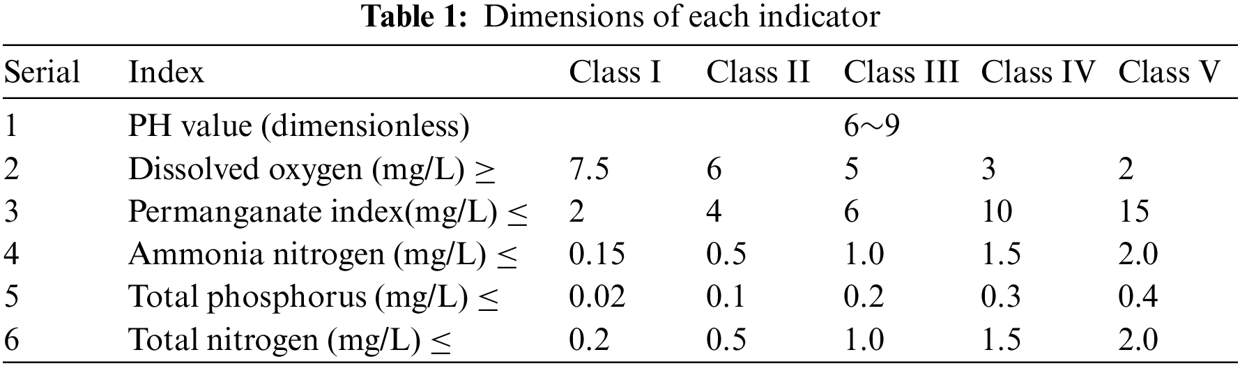
Among them, the permanganate index, ammonia nitrogen, TP and total nitrogen are collected every 4 h, and the other five indicators are collected every hour. We select the TP index as the research object. The raw data crawled from 2019 to 2020 are shown in Tab. 2.

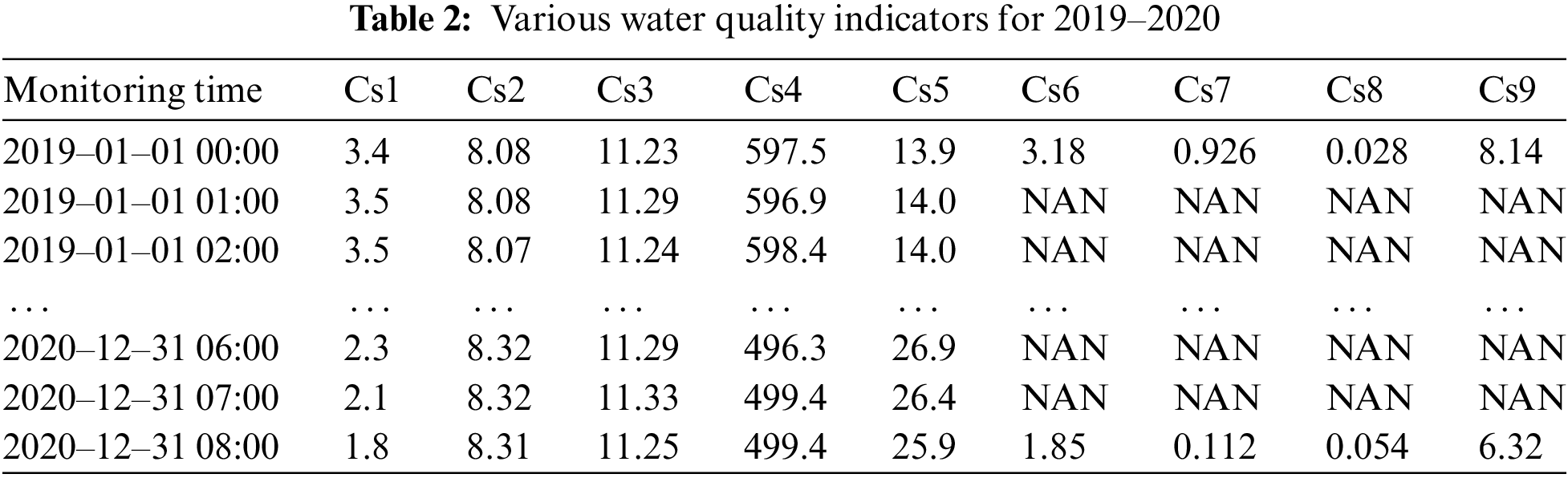
As shown in Tab. 2, there are some missing values in the water quality data. The missing values are handled by using linear interpolation. The missing data processing flow is shown in Fig. 1.

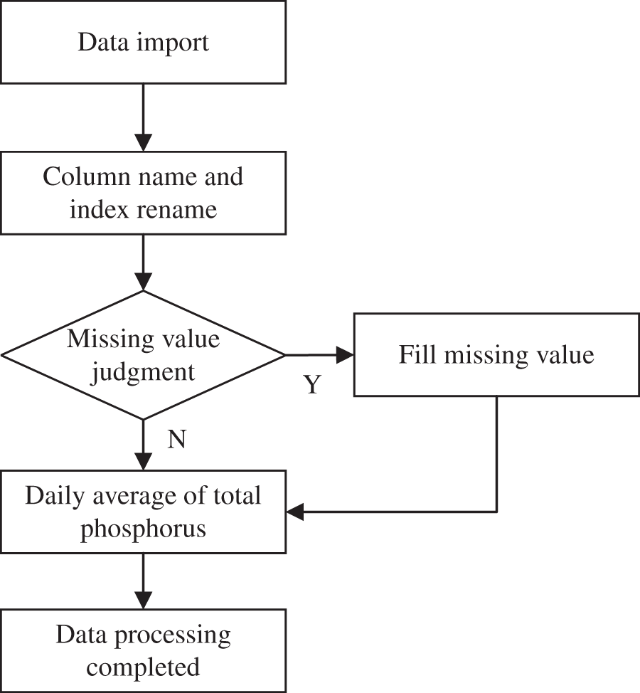
Figure 1: The missing data processing flow chart

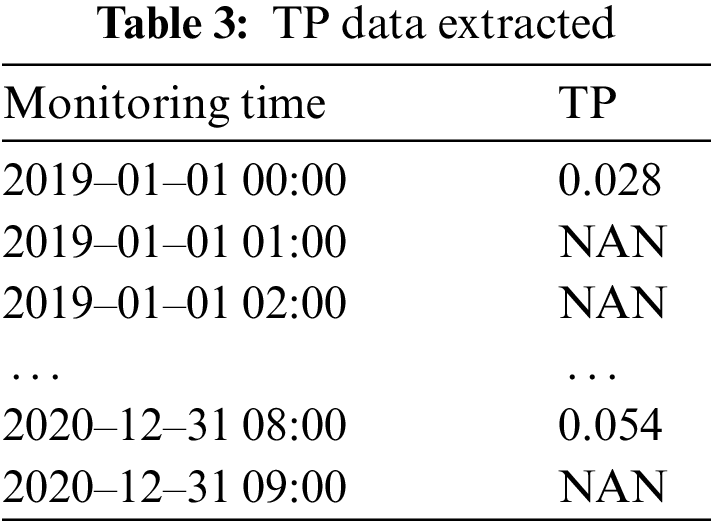
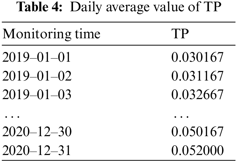
Firstly, import the 2019–2020 TP data, as shown in Tab. 3. Secondly, rename the column name and index. Thirdly, determine the missing value, and fill in the data according to whether there is a missing value. Finally, calculate the daily average value of TP. The results are shown in Tab. 4.

4  ARIMA Forecasting

ARIMA modeling mainly includes several steps, such as stationarity test, white noise test, parameter determination and model prediction.

The data from July 1, 2020 to November 9, 2020 was selected in the 2020 dataset. The data of this period is selected because it needs to be consistent with the data set used by the prediction model in the following chapters to form a comparison and predict the TP indicator from November 10, 2020 to November 19, 2020. The time series diagram of total phosphorus from July 1, 2020 to November 9, 2020 is shown in Fig. 2.

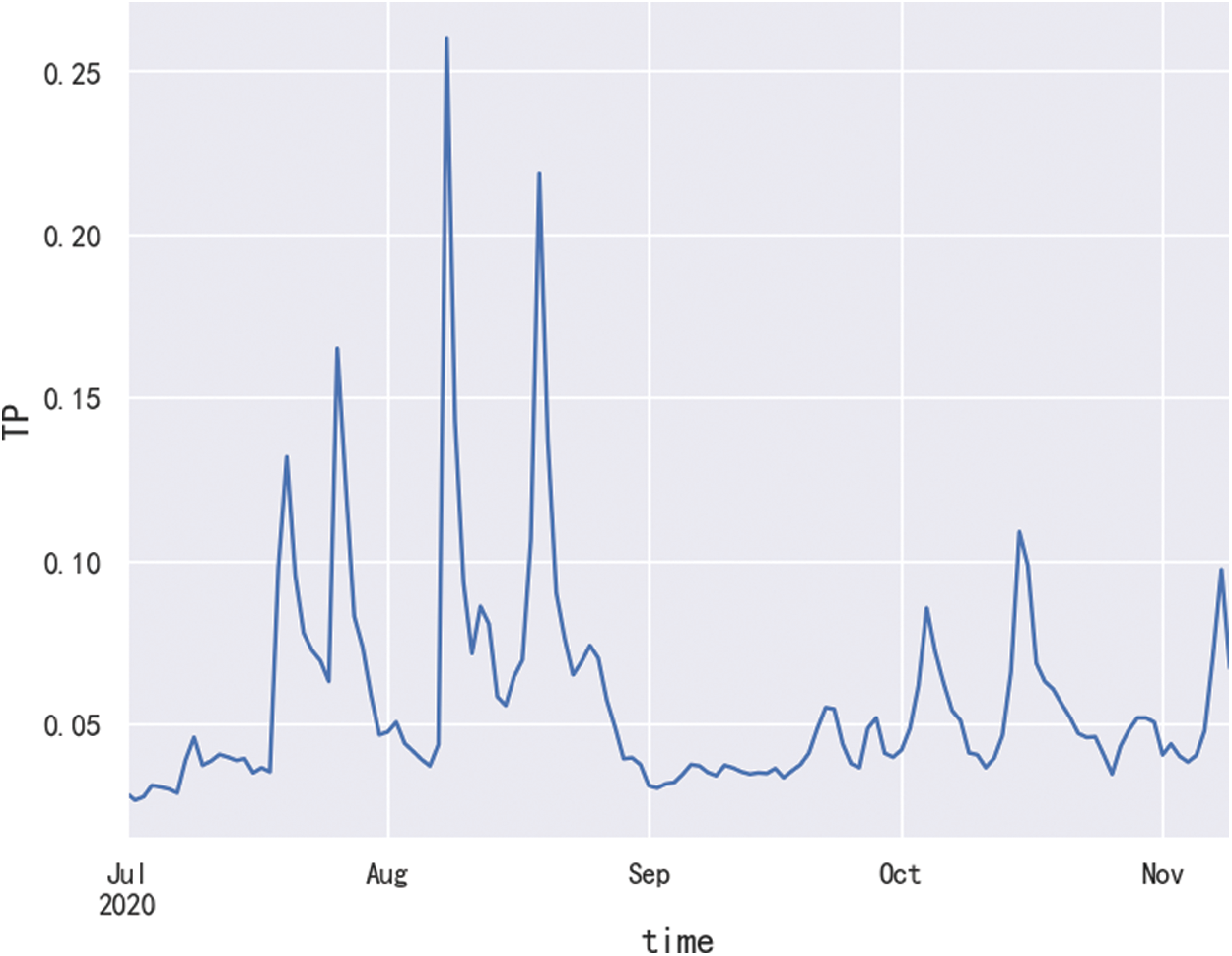
Figure 2: Timing diagram of TP

Stationarity checking. The reason for the stationarity test is that the ARIMA model is used to predict time series data, which must be stable. If the data is unstable, it is impossible to capture the law. The AutoCorrelation Function (ACF) can roughly judge whether the sequence is stationary. With the increase of the delay order, the autocorrelation coefficient of the stationary sequence will quickly decay to zero. The ACF diagram is shown in Fig. 3, and it can be roughly determined that the sequence is a stationary sequence. In order to further determine whether the series is stable, we used the strict statistical test method Augmented Dickey-Fuller (ADF) coefficient to judge. The ADF test is also called unit root test. If the p value of the unit root test is less than 0.05, it is considered to be stable. The ADF coefficient of the current data is: p  = 1.975175e−6, indicating that the data in this period is stationary data, so this period of data does not need to be differentially calculated.

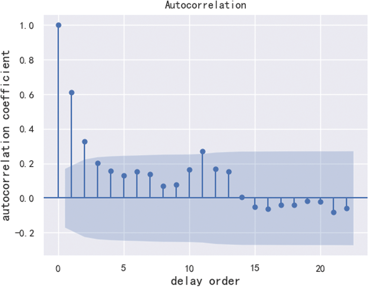
Figure 3: ACF diagram

White noise detecting. After the stationarity checking, it is necessary to perform white noise detecting on the data. The white noise detecting is also called pure randomness test. When the data is pure random data, it is meaningless to analyze the data, so it is best to perform a pure randomness test on the data. It is mainly based on the size of the p value to determine whether it is a random sequence. The p-value is the p-statistic based on the chi-square distribution. If the p-value is less than 0.05, it is considered non-white noise data. The result of the white noise detecting is: p=2.59492822e−12, indicating that the data is non-white noise and can be modeled by ARIMA.

Parameters determining. In order to determine p, q values, the BIC will be used and its calculation formula is:

BIC=−2ln⁡(L)+kln⁡(n)(6)

where k is the number of model parameters, n is the number of samples, and L is the likelihood function. The model evaluation criterion is that the lower the BIC value, the better. When p and q are larger, there are more parameters and k is larger. So making k, p and q smaller, guarantees a better model. By setting the maximum and minimum values of p and q, and then traversing different p and q, the BIC heatmap is obtained, as shown in Fig. 4. According to the minimum BIC principle, we chose p  = 1 and q = 0. At this time BIC is-566.11, and its value is the smallest.

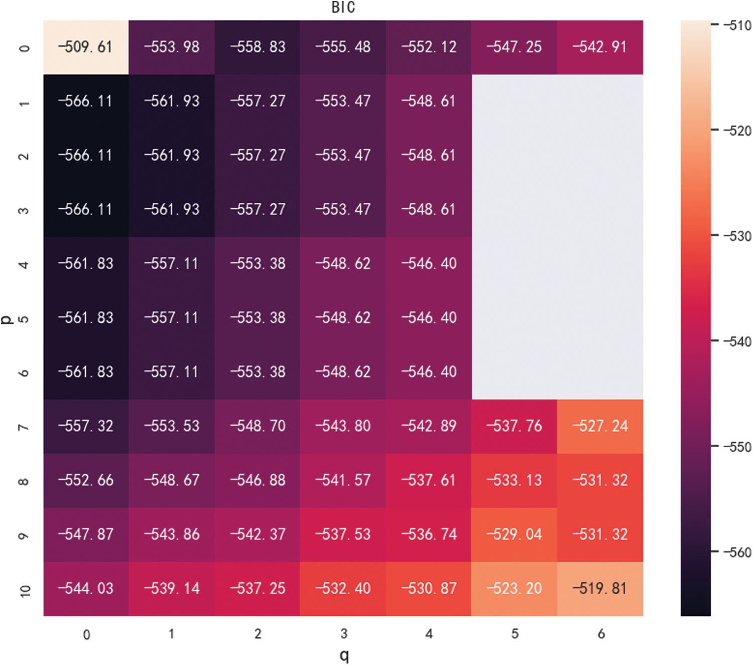
Figure 4: Heatmap order determination

The obtained ARIMA (1,0,0) model is used to fit the data, and the fitting result is shown in Fig. 5. As can be seen from Fig. 5, the model has achieved good results in fitting the data.

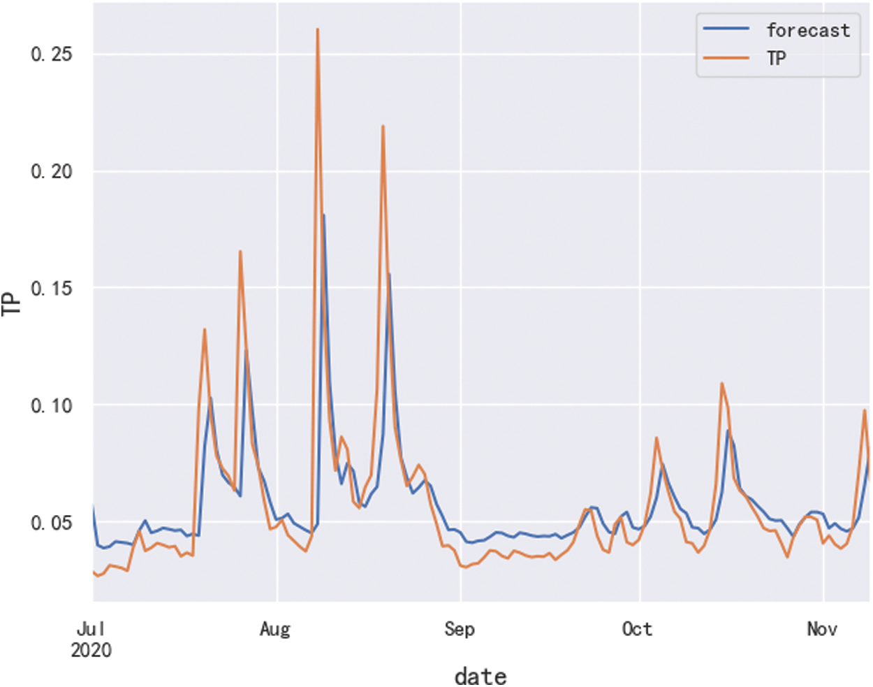
Figure 5: Fitting effect diagram

By using the data from July 1, 2020 to October 20, 2020 as the training set, and the data from October 21, 2020 to November 9, 2020 as the test set, we used the ARIMA (1, 0, 0) model to predict the TP index and the result is shown in Fig. 6. As can be seen from Fig. 6, the prediction effect of sample data is relatively general, and its confidence interval is 95%.

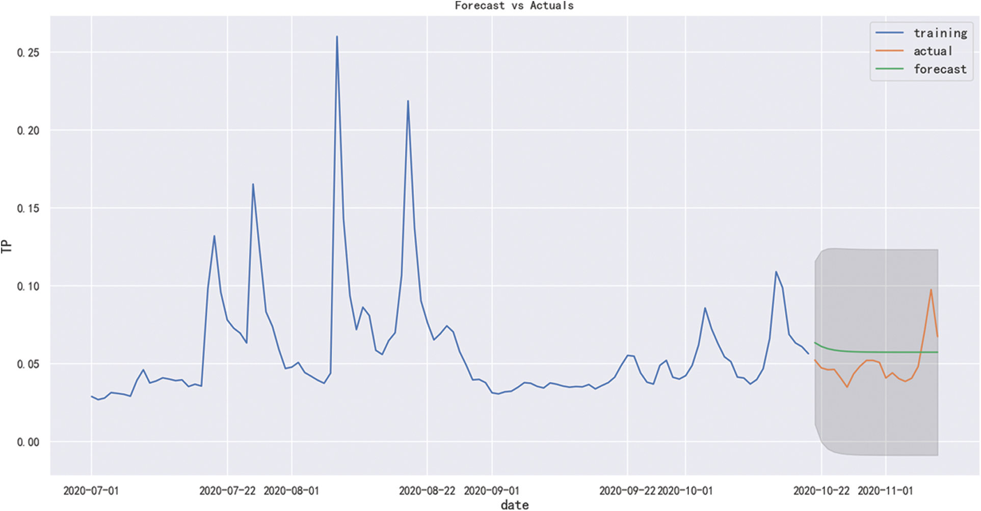
Figure 6: In-sample prediction effect diagram

Finally, the model is used for out-of-sample predictions, and the prediction result is shown in Fig. 7. It can be seen that the model cannot accurately predict the change trend of the actual data, so the ARIMA model has not an ideal prediction effect on the data in this period.

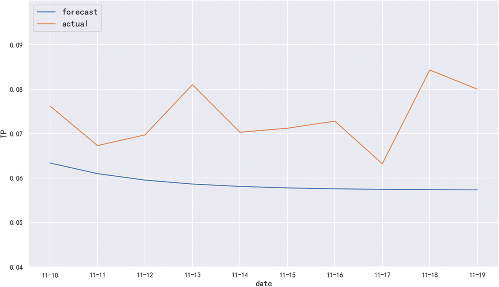
Figure 7: Out-of-sample prediction effect diagram

In order to further analyze the prediction effect of the ARIMA model, we calculated the commonly used evaluation indicators MAE, MSE, MAPE, and the results are shown in Tab. 5.

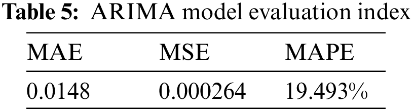
It can also be seen from the evaluation indicators that using the ARIMA model to predict the TP index, its prediction accuracy is not high. This is because the ARIMA model only extracts the trend component characteristics of water quality changes, but cannot extract the random change features. To this end, we intend to analyze the random effect of monitoring water precipitation on TP indicators to extract the random characteristics of TP changes.

5  K-means Cluster Analysis and Correlation Analysis

We did a cluster analysis on the TP data in 2020, and the results are shown in Fig. 8. The data set is divided into four clusters as a whole. The first centroid is 0.0267, there are 172 TP indicators in this cluster, and the overall data range is roughly 0.02 to 0.035; the second centroid is 0.0449, there are 138 TP indicators in this cluster, and the data is roughly between 0.036 and 0.065; the third centroid is 0.0864, there are 49 TP indicators in this cluster, and the index range is roughly between 0.066 and 0.15; the centroid of the fourth cluster is 0.231, and the data metrics range above 0.16. Through the cluster analysis, it can be seen that the TP data is distributed between 0.02 and 0.065 most of the time, but a small amount of data is also distributed outside this range. It seems that other factors influenced the trend of the TP indicator data. Therefore, we decided to analyze the impact of rainfall near the monitoring water area on the TP index.

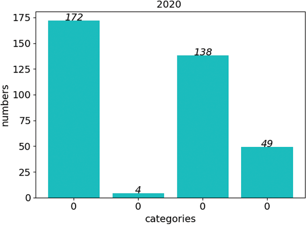
Figure 8: Cluster analysis results of TP index

In order to test our hypothesis, according to the rainfall data crawled from a statistical yearbook (http://tjj.xa.gov.cn/), the rainfall data in 2019 in seven regions near the basin is shown in Tab. 6, and the monthly sum of the TP is added to the end of the table. It can be seen from Tab. 6 that the rainfall period in the basin is concentrated from August to October in 2019, and the monthly sum of the TP is also relatively high in the same period. Therefore, it is particularly necessary to analyze the correlation between the TP data and the rainfall data.

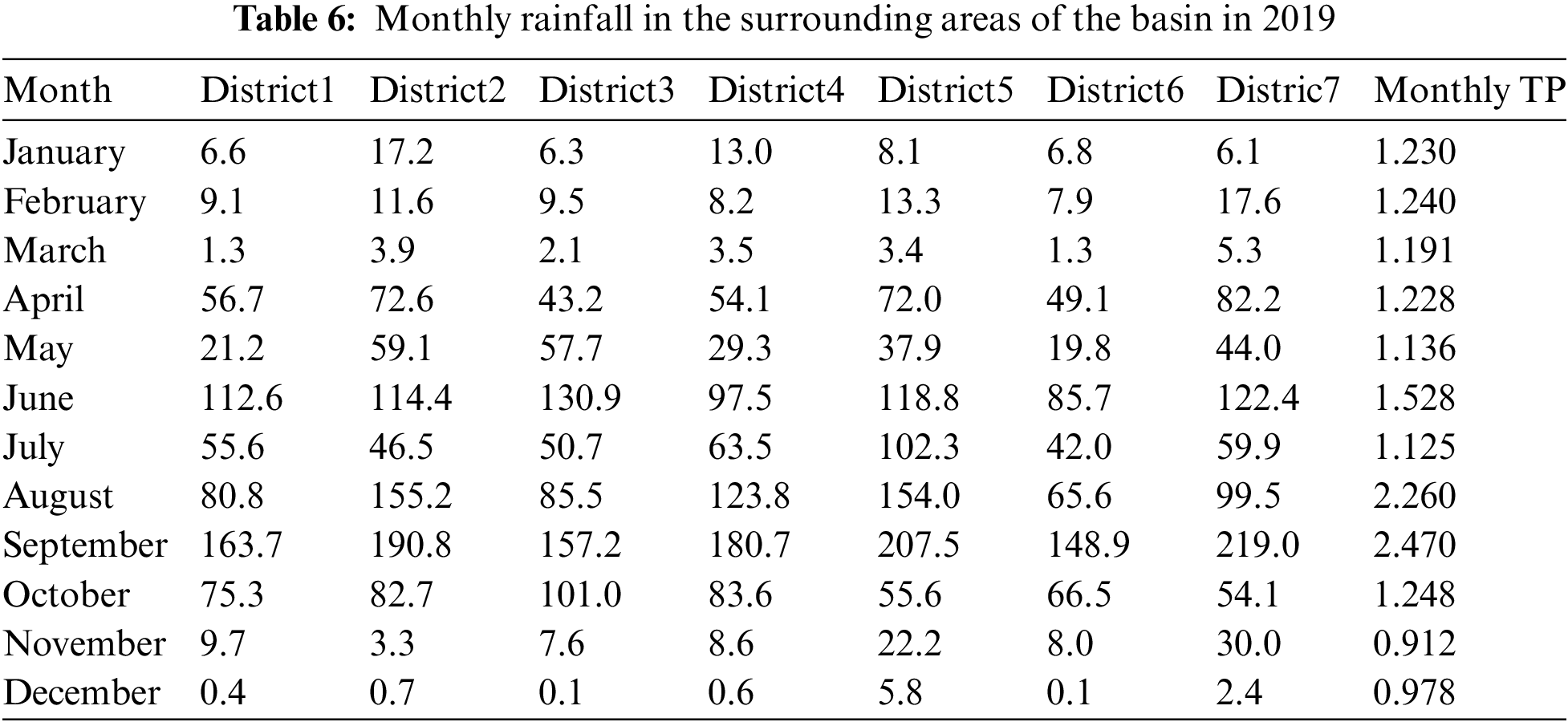
From Tab. 6, we knew that precipitation is positively correlated with TP, so we superimposed the rainfall data and the TP data from July 2020 to December 2020, and the time series diagram is shown in Fig. 9. The rainfall data was downloaded from a rainfall statistics website (http://www.wheata.cn/). According to the time series diagram, it can be observed that when rainfall increases, the value of TP also increases.

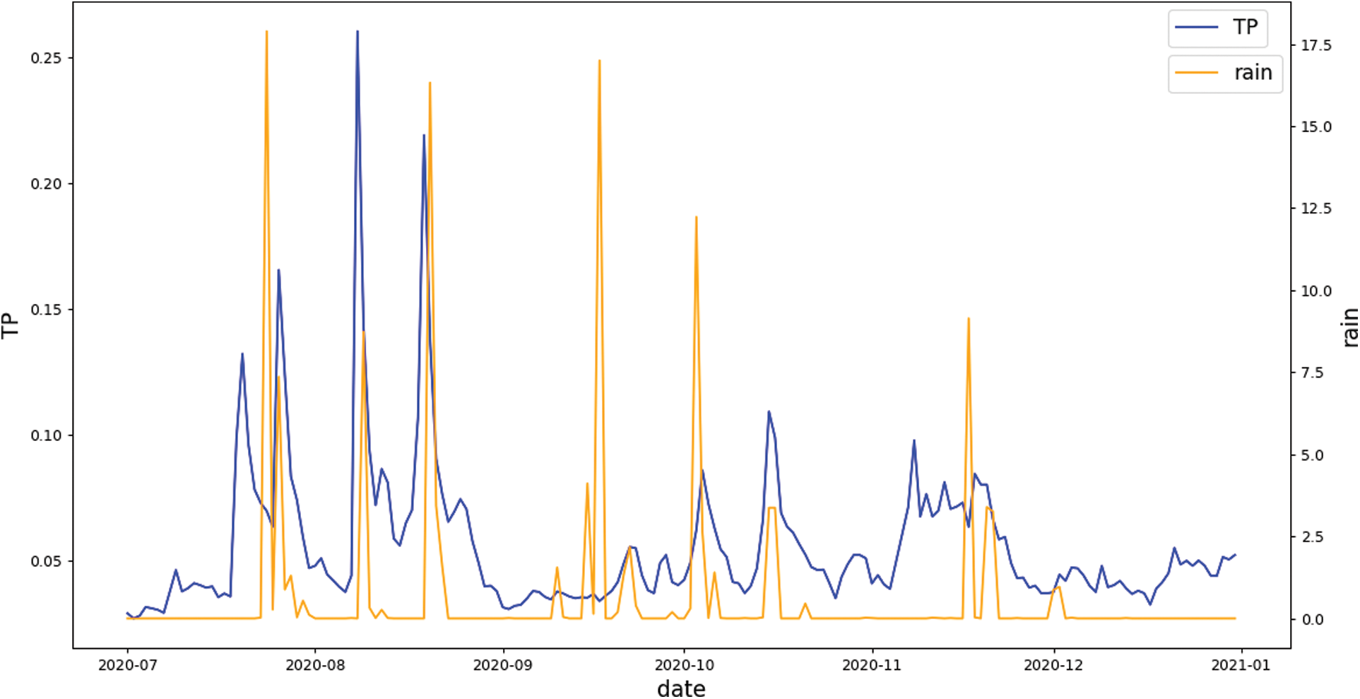
Figure 9: Time series diagram of rainfall and TP

By analyzing the correlation analysis between the monthly rainfall increment data and the monthly TP increment data in 2019, we got that the correlation score was 0.82, and the regression line is shown in Fig. 10. Its first-order equation is:

y=−0.0359+0.00699x(7)

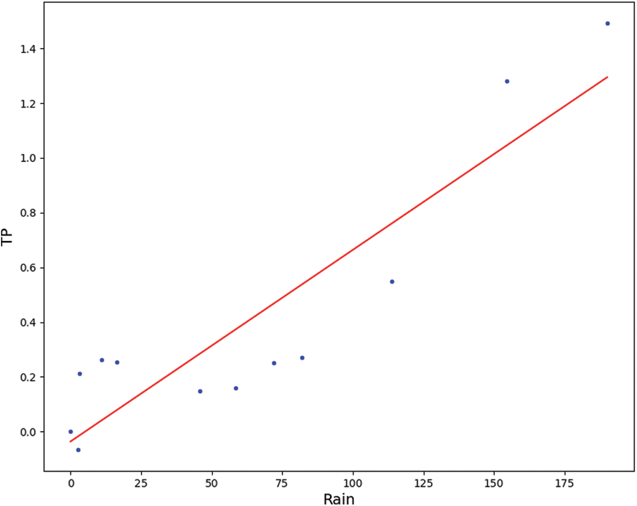
Figure 10: First-order linear regression of TP and monthly rainfall

Therefore, according to this correlation analysis, it can be seen that there is a strong correlation between rainfall increment and TP increment.

6  Combining ARIMA and Clustering for Prediction

Since rainfall can affect the TP index, the selection of the dataset needs to take the rainfall data into account. By using the ARIMA model combined with the clustering model to predict the data from November 10, 2020 to November 19, 2020, and the prediction result is shown in Fig. 11. The predicted value of the TP index is close to the change trend of the actual data during this period.

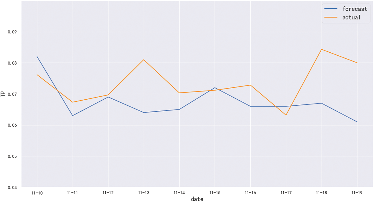
Figure 11: The prediction effect of ARIMA model combined with clustering model

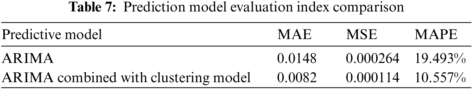
In order to further analyze the prediction effect of this model, we used the commonly used evaluation indicators MAE, MSE, MAPE to analyze the prediction results of the ARIMA model, and the results are shown in Tab. 7. As can be seen from Tab. 7, compared with the ARIMA model, the value of MAE decreased from 0.0148 to 0.0082, MSE decreased from 0.000264 to 0.000114, and MAPE decreased from 19.493% to 10.557%. Therefore, the prediction effect of ARIMA model combined with clustering model is more accurate, and the forecast error is smaller. So it has greater practical significance in the prediction of the water quality.

7  Conclusion

The traditional time series ARIMA model has great prediction effect on data with trend characteristics, but has poor prediction effect on data with random characteristics. Due to the trend and randomness of the changes of the water quality TP data, by combining the ARIMA model and the clustering model, this paper proposed a water quality predicting method combining the ARIMA model and the clustering model based on the characteristics of trend components and random increments. The experimental results show that its prediction accuracy is significantly higher than that of the single ARIMA model. However, the model also has some shortcomings. When predicting the TP index, the accurate rainfall data must be also required. Due to weather forecasts or other reasons, the inaccurate rainfall data will also affect the proposed model’s predicting accuracy. Subsequent studies will take into account the geographical location, time and space of the basin to improve the accuracy of prediction.

Acknowledgement: The authors would like to appreciate all anonymous reviewers for their insightful comments and constructive suggestions to polish this paper in high quality.

Funding Statement: This research was funded by the National Natural Science Foundation of China (No. 51775185), Natural Science Foundation of Hunan Province (2022JJ90013), Scientific Research Fund of Hunan Province Education Department (18C0003), Research project on teaching reform in colleges and universities of Hunan Province Education Department (20190147), and Hunan Normal University University-Industry Cooperation. This work is implemented at the 2011 Collaborative Innovation Center for Development and Utilization of Finance and Economics Big Data Property, Universities of Hunan Province, Open project, Grant Number 20181901CRP04.

Conflicts of Interest: The authors declare that they have no conflicts of interest to report regarding the present study.

References

 1.  Y. K. Hu, N. Wang, S. Liu, Q. L. Jiang and N. Zhang, “Application research of time series model and LSTM model in water quality prediction,” Journal of Chinese Computer Systems, vol. 42, no. 8, pp. 1569–1573, 2021. [Google Scholar]

 2.  J. Zhang, Y. Sheng, W. Chen, H. Lin, G. Sun et al., “Design and analysis of a water quality monitoring data service platform,” Computers, Materials & Continua, vol. 66, no. 1, pp. 389–405, 2021. [Google Scholar]

 3.  G. Sun, F. H. Li and W. D. Jiang, “Brief talk about big data graph analysis and visualization,” Journal on Big Data, vol. 1, no. 1, pp. 25–38, 2019. [Google Scholar]

 4.  B. Yang, L. Xiang, X. Chen and W. Jia, “An online chronic disease prediction system based on incremental deep neural network,” Computers, Materials & Continua, vol. 67, no. 1, pp. 951–964, 2021. [Google Scholar]

 5.  Y. Sheng, J. Zhang, W. Tan, J. Wu, H. Lin et al., “Application of grey model and neural network in financial revenue forecast,” Computers, Materials & Continua, vol. 69, no. 3, pp. 4043–4059, 2021. [Google Scholar]

 6.  J. H. Xu, J. C. Wang, L. Chen and Y. Wu, “Prediction model of surface water quality based on graph neural network,” Journal of Zhejiang University (Engineering Science), vol. 55, no. 4, pp. 601–607, 2021. [Google Scholar]

 7.  X. K. Luo, Y. X. He, P. Liu and W. Li, “Application of ARIMA-SVR combination method in water quality prediction,” Journal of Changjiang Academy of Sciences, vol. 37, no. 10, pp. 21–27, 2020. [Google Scholar]

 8.  J. Wang, L. Y. Zhang, W. Zhang and X. D. Wang, “Reliable model of reservoir water quality prediction based on improved ARIMA method,” Environmental Engineering Science, vol. 36, no. 9, pp. 1041–1048, 2019. [Google Scholar]

 9.  J. Huan, B. Chen, X. G. Xu, H. Li, M. B. Li et al., “River dissolved oxygen prediction based on random forest and LSTM,” Applied Engineering in Agriculture, vol. 37, no. 5, pp. 901–910, 2021. [Google Scholar]

10. Y. Zhang and Q. Q. Gao, “Research on comprehensive water quality prediction model based on grey model and fuzzy neural network,” Chinese Journal of Environmental Engineering, vol. 9, no. 2, pp. 537–545, 2015. [Google Scholar]

11. P. S. Xue, M. Q. Feng and X. P. Xing, “An improved grey neural network water quality prediction model based on markov chain,” Engineering Journal of Wuhan University, vol. 45, no. 3, pp. 319–324, 2012. [Google Scholar]

12. R. Z. Li, “Research progress and trend analysis of water quality prediction theory model,” Journal of Hefei University of Technology, vol. 29, no. 1, pp. 26–30, 2006. [Google Scholar]

13. C. Han, S. Song and C. H. Wang, “Real-time adaptive prediction of short-term traffic flow based on ARIMA model,” Journal of System Simulation, vol. 16, no. 7, pp. 1530–1532, 2004. [Google Scholar]

14. Y. M. Yang, “Prediction of Beijing consumer price index based on ARIMA model,” Statistics & Decision, vol. 31, no. 4, pp. 76–78, 2015. [Google Scholar]

15. Z. D. Tian, S. J. Li and Y. H. Wang, “Gaussian process regression compensated ARIMA for network traffic prediction,” Journal of Beijing University of Posts and Telecommunications, vol. 40, no. 6, pp. 65–73, 2017. [Google Scholar]

16. J. G. Sun, J. Liu and L. Y. Zhao, “Research on clustering algorithm,” Journal of Software, vol. 19, no. 1, pp. 48–61, 2008. [Google Scholar]

17. X. B. Yang, “Research on some key technologies in cluster analysis,” M.S. theses, Zhejiang University, Hangzhou, China, 2005. [Google Scholar]

18. J. C. Yang and C. Zhao, “A review of k-means clustering algorithm research,” Computer Engineering and Applications, vol. 55, no. 23, pp. 7–14, 2019. [Google Scholar]

19. W. D. Jiang, J. Wu, G. Sun, Y. X. Ouyang, J. Li et al., “A survey of time series data visualization methods,” Journal of Quantum Computing, vol. 2, no. 2, pp. 105–117, 2020. [Google Scholar]

20. G. H. Zhao, “Research on stock price trend prediction based on time series analysis,” M.S. theses, Xiamen University, Xiamen, China, 2009. [Google Scholar]

21. L. Xia, “Research on regional electricity consumption prediction method based on ARIMA model and regression analysis,” M.S. theses, Nanjing University of Science and Technology, Nanjing, China, 2013. [Google Scholar]

22. R. H. Shumway and D. S. Stoffer, “ARIMA model,” in Time Series Analysis and Its Applications: With R Examples, Fourth Edition, 4th ed., Beijing, China: Machinery Industry Press, pp. 63–134, 2020. [Google Scholar]

23. X. D. Wu, V. Kumar, J. R. Quinlan, J. Ghosh, Y. Qiang et al., “Top 10 algorithms in data mining,” Knowledge and Information Systems, vol. 14, no. 1, pp. 1–37, 2008. [Google Scholar]

24. H. T. Peng, “Research on power generation forecast based on GM-ARIMA model,” M.S. theses, Lanzhou University, Lanzhou, China, 2014. [Google Scholar]