Genetic Crossover Operators for the Capacitated Vehicle Routing Problem

1  Introduction

There are numerous real-life distribution management problems, where constructing delivery route from a headquarters to some customers is very important. If same customers must be provided service very frequently, it is preferred to set up an optimal tour. This problem is called vehicle routing problem (VRP) which is a very challenging optimization problem. It was introduced first in [1] as follows: There is a convoy of vehicles with the same or different capacities in a depot. These vehicles are expected to serve some customers with different demands such that cost of the tours of the vehicles is minimum. The VPR has numerous variants, namely, the VRP with pickup and delivery (VRPPD), the VRP with time window (VRPTW), the VRP with Backhauls (VRPB), the multi-depot VRP (MDVRP), the split delivery VRP (SDVRP), the capacitated VRP (CVRP) [2].

We consider the CVRP for our study. Several researchers extensively studied on the CVRP, where a convoy of vehicles provides services to different customers from a depot (headquarters) so that sum of the routing costs under their capacity constraints is minimized. The CVRP is a mixture of the standard travelling salesman problem (TSP) and the bin packing problem (BPP). The CVRP has applications in many real-life problems, such as renting-sharing problems for urban bicycles [3], scheduling and routing of retail stores [4], dispensing medical supplies [5], etc. The classical CVRP is NP-hard [6] and is a very complicated problem. For example, for a n-customer and m-vehicle problem, we are listing n customers in a sequence (that can be implemented in n! ways), and then placing m–1 constraints to determine when a tour has concluded after (m−1) of (n−1) customers, that can be implemented in (n−1m−1) ways, producing n!(n−1m−1)/m! probable solutions (as the vehicle sequence is irrelevant, we divide by m!). One can visualize that with more than 10 customers and 3 vehicles, there are many solutions. For any size n, the number of feasible solutions is too large; so, an extensive search is too complicated. That is, the problem is too complicated to solve. Various procedures to solve the CVRP were reported in numerous literatures, which are categorized into two major categories–exact methods and heuristic methods. Exact methods, for instance, branch and bound [7], branch and price [8], branch and cut [9], lexisearch algorithm [10], give exact solutions. However, as the problem size increases, finding exact solutions using these methods is very difficult. On the other hand, heuristic methods don’t ensure the exact solutions but give near exact solutions rapidly. The most recent methods which can be applied to several optimization problems are called metaheuristics. Several metaheuristics were proposed to solve this problem. These algorithms are simulated annealing [11], tabu search [12], ant colony optimization [13], particle swarm optimization [14], genetic algorithms [15], variable neighbourhood method [16], etc. However, genetic algorithms (GAs) are observed to be widely used methods amongst latest metaheuristic approaches, and hence, we are using GAs to obtain solution to the CVRP.

Introduced first by John Holland, GAs are proposed according to the survival-of-the-fittest theory amongst various species produced by random differences in the structure of chromosomes in the natural science. Because GAs are easy, flexible and simple to code, they are extremely successful. Generally, GAs start with a chromosome set named initial population. Then mainly three operators, specifically, selection, crossover and mutation, are applied to find solution to any problem. Selection operator selects better chromosomes among the existing chromosomes, crossover operator probabilistically produces new chromosome(s) called offspring(s) by mating two chromosomes, and mutation probabilistically changes some genes in the chromosomes. Among these three operators crossover is very crucial in designing and implementing GAs [17]. Hence, different crossover operators can be applied in GAs for the CVRP which were originally proposed for the TSP. This paper intends to compare the performance of some crossover operators to test the suitability of the operators to solve the CVRP. These operators were originally proposed for the standard TSP. We further aim to determine a comparative rank of the crossovers for the CVRP.

This manuscript is prepared as follows: Section 2 reports definition and model of the CVRP. Section 3 briefly discusses existing literatures for the CVRP using genetic crossover operators. Section 4 discusses GAs using existing crossover operators for the CVRP. Section 5 reports the experimental results of the GAs on some asymmetric and symmetric instances. Section 6 presents a conclusion.

2  Problem Definition: The CVRP

The CVRP can be stated as: Suppose V = {0, 1, 2, . . ., n} be a set of customers (or nodes or cities), ‘customer 0’ is the headquarters and there are m vehicles, each with capacity Q. Each customer i ∈ V, related to a non-negative demand qi, is required to be visited exactly once. The number of vehicles may be predetermined or determined during the process. Also, suppose, C = [cij] be a travel cost (or time or distance) matrix associated with each pair of customers. The matrix C may be symmetric or asymmetric; the latter case is due to the presence of one-way roads in urban areas. The problem is to find an optimal tour that has minimum total arrival cost at n customers utilizing all m vehicles, so that starting from and stopping at the headquarters all customers are to be visited (serviced) just once and the total demand serviced does not exceed vehicle capacity Q [18]. That is, a solution of the CVRP with m routes {R1, R2, . . . , Rm} must satisfy the following equation:

∑i\; ε\; Rjqi≤Q(1)

The CVRP aims to minimize the total cost of the tour, S, described as:

f(S)=∑i,j\; ε\; Vcij(2)

As shown in Fig. 1, the CVRP is concerned with finding the optimal tours for 3 vehicles to fulfill the demands of 10 customers. Note that ‘customer 1’ is the headquarters (depot). The Fig. 1. denotes the tour {1→5→3→ 1→10→8→ 2→7→1→ 6 →4→ 9 →1} of the vehicles. Here, the customers 5 and 3 are served in the order by the 1st vehicle, the customers 10, 8, 2 and 7 are served in the order by the 2nd vehicle, and the customers 6, 4 and 9 are served in the order by the 3rd vehicle.

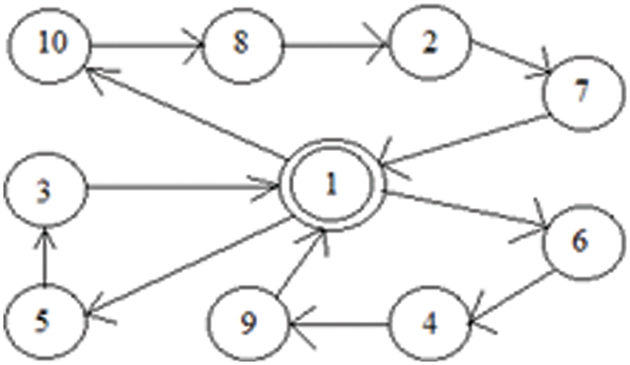
Figure 1: Graphical representation of the CVRP with n = 10 and m = 3

3  Literature Review

We aim to compare the performances of numerous crossover operators to find solution to the CVRP. Therefore, we report a short review on the literatures that applied different crossover operators to find solution to the problem. It is noted that the crossover operators which are designed for the TSP could also be utilized for the CVRP.

In [19], three crossovers operators, namely order crossover (OX), partially mapped crossover (PMX) and uniform crossover (UX), and three mutation operators, namely, swapping, inversion, swapping + inversion, with two types of solution representation, namely, direct coding and indirect coding, for the CVRP are compared. Experimental study on seven instances from a standard set of [20] showed that PMX with inversion mutation had the best performance for direct encoding, and OX with inversion mutation gave best solution values for indirect representation.

In [21], an optimized crossover genetic algorithm (OCGA) is introduced for the VRP with capacity restrictions. The main feature of the algorithm was that vehicles with similar capacities located in a depot were used in a way to optimize the routes and satisfy the demands of the customers. The proposed algorithm used an optimized crossover operator that employed a directed complete bipartite graph for finding an optimal set of delivery routes, to satisfy demands and minimize the total costs. The experimental results indicated that the algorithm is competitive.

In [22], a comparative study among eight crossover operators is reported for the VRP. The crossovers are OX, PMX, alternating edges crossover (AEX), edge recombination crossover (ERX), cycle crossover (CX), heuristic greedy crossovers (HGreX), heuristic probabilistic crossover (HProX) and heuristic random crossover (HRndX). It is reported that HGreX and AEX are competing and are found to be very good operators.

In [23], some crossover operators are applied for solving the CVRP. Further, they proposed a new crossover operator named sinusoidal motion crossover (SMC) and demonstrated it with two examples.

In [24], a giant tour best cost crossover (GTBCX) for the CVRP is proposed. Further, a non-dominated sorting GA-II (NSGA-II) utilizing GTBCX is proposed to optimize two objective values in the CVRP, i.e., the overall distance travelled by the given fleet of vehicles and the length of the longest route.

In [25], the sequential constructive crossover (SCX) is developed for the usual TSP and then utilized for other related problems.

In general, there are two kinds of crossover operators available in the literature. One is the distance-based crossover, and another is the blind crossover. The distance-based crossovers consider distances among customers (or cities or nodes) and the blind crossovers do not consider any data related to the problem instance. The comparison will not be fair if the effectiveness of the distance-based crossover is evaluated against the blind crossovers [26]. So, we consider four blind crossovers, namely, OX, PMX, CX and AEX, and four distance-based crossovers, namely, heuristic crossover (HX), greedy crossover (GX), modified HX (MHX) and SCX for our comparative study. Illustration of these crossover operators are reported for a pair of parent chromosomes. Further, these crossover operators without mutation and with mutation operators are encoded in Visual C++ and then experimented on some benchmark instances with different sizes and various number of vehicles. Our investigation indicates the superiority of the SCX for this problem.

4  GAs for the CVRP

The aim of this current study is to evaluate the performance of various crossover operators in GAs for the CVRP. Therefore, the general structure of the developed GA is selected to differentiate the performance of the compared crossover operators.

4.1 Chromosome Representation and Initial Population

To apply GA to solve any optimization problem, a representation of a solution as chromosome should be defined initially. In our GAs, an integer chromosome using path representation is considered whose length is n + m − 1, where n and m be the numbers of customers and vehicles respectively. In this representation, additional m − 1 customers representing dummy depots are added to represent the starting of tours by new vehicles [27]. Fig. 2a displays an example chromosome (1, 6, 9, 8, 5, 2, 10, 4, 3, 7) and its corresponding tour {1→6→9→ 8→5→2→ 10→4→3→7 →1} with 9 customers and 2 vehicles, where the integers 1 and 10 are the depots, the others are customers. Fig. 2b shows the routes {1→6→9→ 8→5→2→ 1} and {1→4→3→7 →1} of the 1st and 2nd vehicles respectively, and their graphical versions are displayed in Fig. 2c. It means that the customers 6, 9, 8, 5 and 2 are served in the order by the 1st vehicle, and the customers 4, 3 and 7 are served in the order by the 2nd vehicle. Therefore, the given cost matrix should be augmented for showing the dummy depots. For this reason, (m − 1) copy of the depot (customer 1) column and row (i.e., 1st column and 1st row) are attached to the original given cost matrix.

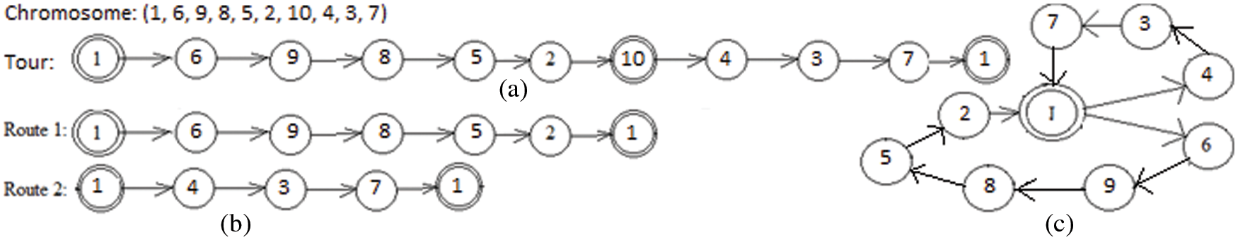
Figure 2: (a) A chromosome example, (b) the CVRP routes and (c) the graphical version

The initial population of chromosomes of predefined size (Ps) is created arbitrarily as in Algorithm 1.

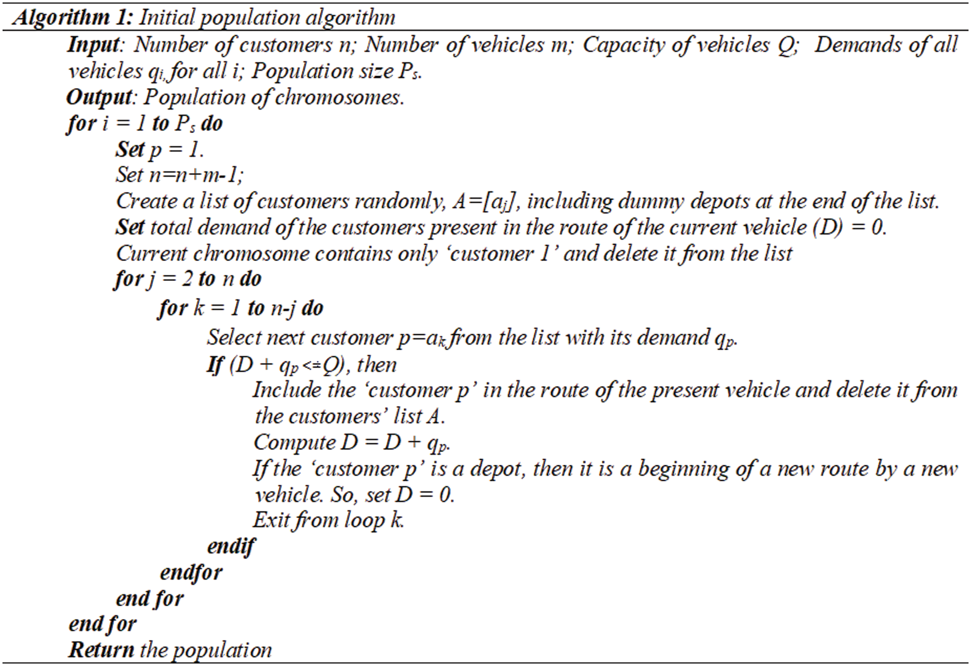
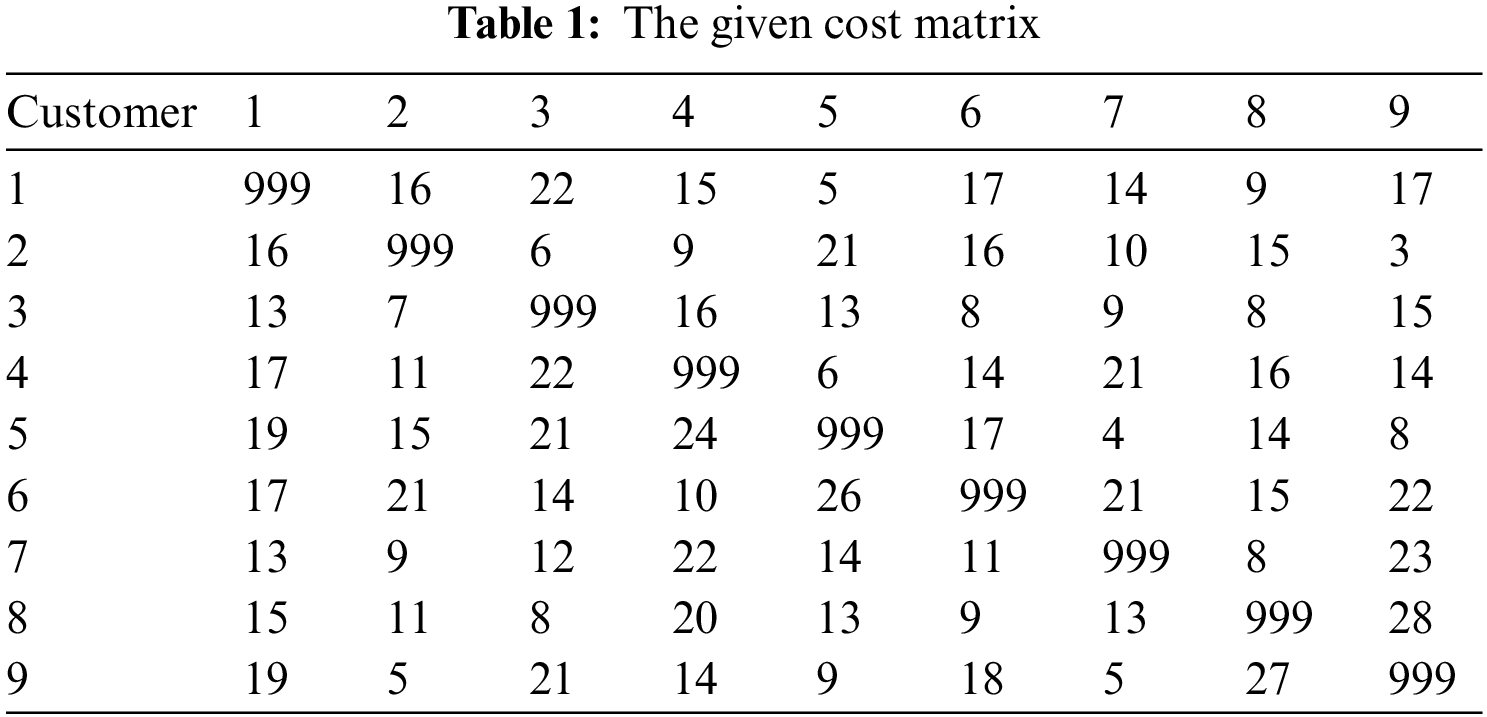
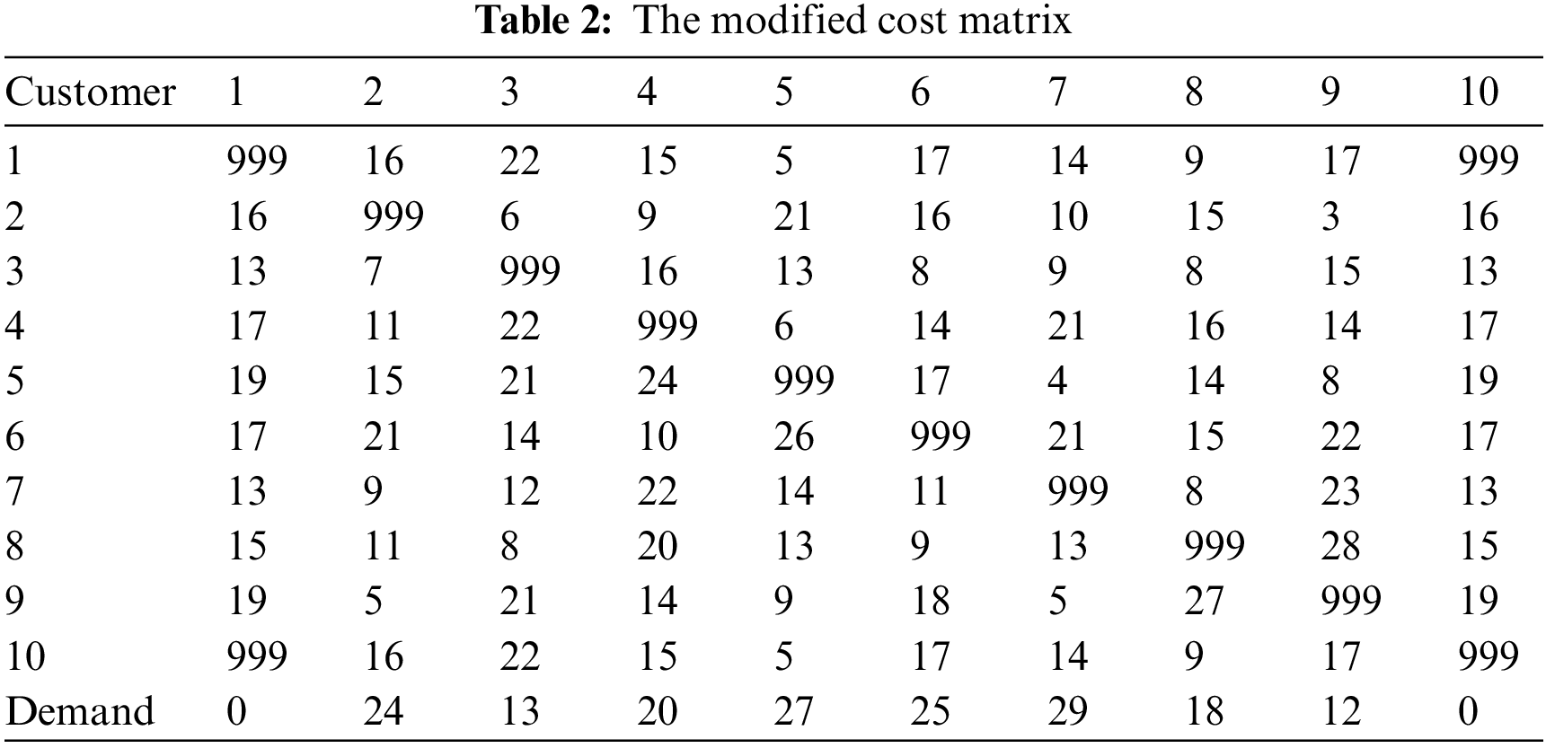
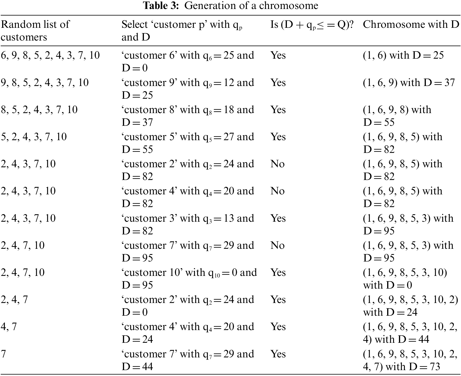
We illustrate a chromosome generation through the 9 customers and 2 vehicles with given matrix (Tab. 1). We modify the given cost matrix by combining a copy of headquarters (customer 1) column and row (i.e., 1st column and 1st row) to the matrix [28] (Tab. 2). Given the capacity of every vehicle, Q = 100. Further, demands of the customers are given in the Tab. 2. Tab. 3 shows the generation of the chromosome (1, 6, 9, 8, 5, 3, 10, 2, 4, 7). Similarly, a population of chromosomes is generated.

4.2 Chromosome Evaluation and Selection Operator

The objective function value of a chromosome (solution) is the total service cost of the routes by all vehicles. The cost of every route is the addition of the service costs among the customers. Since the CVRP is a minimization problem, so, the fitness function, fi, is the inverted objective function, that is,

fi=11+oi;oiistheobjectivefunctionvalueofithchromosome(3)

In selection operator, a subpopulation (some chromosomes) is selected from the existing population for producing the next population. The performance of GA depends on selection operator without which GA is same as random sampling that produces different results in the generations. Several selection procedures exist in the literature. For our GAs, the fitness proportional selection (FPS) using roulette wheel selection (RWS) [17] is applied. The RWS is widely used method where the fitness of every chromosome is related to the area of roulette wheel portion. Then, the roulette wheel is rotated and the chromosome, which is pointed by the wheel pointer, is selected for next generation mating pool. Based on the fitness of each chromosome, a probability pi of selection is calculated as follows:

pi=fi∑j=1Psfj;i∈{1,2,……,Ps}(4)

where Ps is the population size. Thus, fitter chromosomes have greater chance of being selected as parents. During the selection procedure, there is no change of the segment size and selection probability. This procedure is very easy to implement that provides unbiased distributed probabilities to the chromosomes and allocates higher probability to the best chromosome.

4.3 Crossover Operators

The selection process provides a consistency between exploration and exploitation of search area. The crossover is the most important process in GAs that is implemented on a chromosome pair to produce offspring(s). Selection and crossover operators together can speed up the convergence of GAs. The fundamental crossover operators cannot produce feasible offspring(s) for the CVRP. The crossover operators which were designed for the usual TSP can be implemented to the CVRP. As the blind crossovers and the distance-based crossover operators are two major kinds of crossover operators, we propose to utilize some of them and then compare them.

4.3.1 Partially Mapped Crossover (PMX) Operator

In [29], the PMX is developed, that describes an exchange mapping in the segment between two selected points. It was the first designed crossover in GA for the TSP. As an example, we choose two parent chromosomes P1: (1, 6, 9, 8, 5, 3, 10, 2, 4, 7) and P2: (1, 8, 6, 9, 4, 3, 10, 7, 5, 2) with costs 172 and 148 respectively (for costs, see Tab. 2). These same parent chromosomes will be used for demonstrating all crossovers here. It is to be noted that crossover operators are applied on the parents after omitting the dummy depots. So, after omitting the dummy depots, we consider the parents: P1: (1, 6, 9, 8, 5, 3, 2, 4, 7) and P2: (1, 8, 6, 9, 4, 3, 7, 5, 2) Once offsprings are created, dummy depots are inserted into them such that capacity constraint is preserved.

Further, we set headquarters (1st gene) as ‘customer 1’. Assume that the arbitrarily selected cut points are between 2nd and 3rd genes, and between 6th and 7th genes which are shown by “|”.

P1: (1, 6 | 9, 8, 5, 3 | 2, 4, 7) and P2: (1, 8 | 6, 9, 4, 3 | 7, 5, 2).

The first gene is always ‘customer 1’. The mapping segments are between these cut points, and the systems are 9↔6, 8↔9, 5↔4, and 3↔3. These segments are copied in offsprings as below:

O1: (1, * | 9, 8, 5, 3 | *, *, *) and O2: (1, * | 6, 9, 4, 3 | *, *, *).

We add other genes from the alternative parents that do not lead to infeasible chromosome:

O1: (1, * | 9, 8, 5, 3 | 7, *, 2) and O2: (1, * | 6, 9, 4, 3 | 2, *, 7)

The 1st * in the 1st offspring would be 8 which is from 2nd parent, however, it is already available in the offspring, so we consider 9 using the map 8↔9, but 9 is also available in the offspring, so, we add 6 using the map 9↔6. Similarly, the 2nd * in that offspring would be 5 which is from 2nd parent, however, it is available in the offspring, so we add 4 using the map 5↔4. So, the 1st offspring leads to O1: (1, 6, 9, 8, 5, 3, 7, 4, 2). Likewise, the 2nd offspring is created as: O2: (1, 8, 6, 9, 4, 3, 2, 5, 7).

Next, we add dummy depots at the end of the offspring chromosomes. Then offsprings become: O1: (1, 6, 9, 8, 5, 3, 7, 4, 2, 10) and O2: (1, 8, 6, 9, 4, 3, 2, 5, 7, 10). Then calculate total demand of the customers. We have for O1, (q1 + q6 + q9 + q8 + q5 + q3) = 0 + 25 + 12 + 18 + 27 + 13 = 95. Now if we add q7 = 29, then 95 + 29 = 124 > 100 (=Q), hence, we exchange ‘customer 7’ with ‘customer 10’. So, the first offspring leads to O1: (1, 6, 9, 8, 5, 3, 10, 4, 2, 7) with cost 162. Likewise, the 2nd offspring is created as: O2: (1, 8, 6, 9, 4, 3, 10, 5, 7, 2) with cost 123.

4.3.2 Ordered Crossover (OX) Operator

In [30], the OX is designed that creates offspring by selecting a segment of a tour from one parent and maintaining the relative sequence of customers from the other one. Consider the following same parents with two cut points shown by “|”:

P1: (1, 6 | 9, 8, 5, 3 | 2, 4, 7) and P2: (1, 8 | 6, 9, 4, 3 | 7, 5, 2)

We always fix first gene as ‘customer 1’. First, we copy the genes between two cut points to the offspring as:

O1: (1, * | 9, 8, 5, 3 | *, *, *) and O2: (1, * | 6, 9, 4, 3 | *, *, *)

Next, starting from 2nd cut point of one parent, genes from other one, excluding existing ones, are copied by maintaining sequence. The order of genes in 2nd parent from 2nd cut point is “7→5→2→8→6→9→4→3.” After excluding existing genes 9, 8, 5 and 3, the order becomes “7→2→6→4”, that is put in 1st offspring starting from 2nd cut point as: O1: (1, 4 | 9, 8, 5, 3 | 7, 2, 6). Similarly, we build the second offspring as: O2: (1, 5 | 6, 9, 4, 3 | 2, 7, 8).

Next, we add dummy depots at the end of the offspring chromosomes. Then offsprings become: O1: (1, 4, 9, 8, 5, 3, 7, 2, 6, 10) and O2: (1, 5, 6, 9, 4, 3, 2, 7, 8, 10). Then calculate total demand of the customers. We have for O1, (q1 + q4 + q9 + q8 + q5 + q3) = 0 + 20 + 12 + 18 + 27 + 13 = 90. Now if we add q7 = 29, then 90 + 29 = 119 > 100 (=Q), hence, we exchange ‘customer 7’ with ‘customer 10’. So, the first offspring becomes O1: (1, 4, 9, 8, 5, 3, 10, 2, 6, 7) with cost 169. Similarly, we build the second offspring as: O2: (1, 5, 6, 9, 4, 3, 10, 7, 8, 2) with cost 142.

4.3.3 Alternating Edges Crossover (AEX) Operator

In [31], the AEX is proposed, that presumes chromosome as a directed cycle of arcs. It produces only one offspring by choosing alternative arcs from the parents. However, in case of infeasibility, random gene is added to the offspring. Consider the following same parents: P1: (1, 6, 9, 8, 5, 3, 2, 4, 7) and P2: (1, 8, 6, 9, 4, 3, 7, 5, 2).

Initially, the arc (1, 6) is chosen from 1st parent and copied to the offspring. Then arcs (6, 9) from 2nd one, and (9, 8) from 1st one, are chosen and copied to the offspring. Next, since the chosen arc (8, 6) from 2nd one makes a cycle, so, a random arc (8, 2) is chosen. Later, the arcs (2, 4) from 1st parent and (4, 3) from 2nd one, are chosen and copied to the offspring. Finally, the arcs (3, 5) and (5, 7) are chosen randomly. This way the following offspring is created: O: (1, 6, 9, 8, 2, 4, 3, 5, 7).

Next, we add dummy depots at the end of the offspring chromosome which becomes: O: (1, 6, 9, 8, 2, 4, 3, 5, 7, 10). Then calculate total demand of the customers. So, we have, (q1 + q6 + q9 + q8 + q2 + q4) = 0 + 25 + 12 + 18 + 24 + 20 = 99. Now if we add q3 = 13, then 99 + 13 = 112 > 100 (=Q), hence, we exchange ‘customer 3’ with ‘customer 10’. Finally, the offspring leads to O: (1, 6, 9, 8, 2, 4, 10, 5, 7, 3) with cost 137.

4.3.4 Cycle Crossover (CX) Operator

In [32], CX is developed, which creates an offspring where each gene and its related position derived from any parent. Consider the same example parent chromosomes P1: (1, 6, 9, 8, 5, 3, 2, 4, 7) and P2: (1, 8, 6, 9, 4, 3, 7, 5, 2).

The first position in the offspring 1, for 2nd position, we choose ‘customer 6’ from 1st parent, then the 1st offspring leads to: O1: (1, 6, *, *, *, *, *, *, *).

In the offspring, each gene is selected from any parent with the same location, so gene 8 must be considered, since gene 8, in 2nd parent, is below gene 6. In 1st parent, gene 8 is at 4th location; so, the offspring leads to: O1: (1, 6, *, 8, *, *, *, *, *).

Next, we select gene 9 as, in 2nd parent, it is below gene 8. In 1st parent, gene 9 is at 3rd location; so, the offspring leads to: O1: (1, 6, 9, 8, *, *, *, *, *).

Next, we select gene 6 as, in 2nd parent, it is below gene 9. However, it leads to a cycle. So, we fill up the empty positions by the genes available in corresponding positions in 2nd parent. So, the offspring leads to: O1: (1, 6, 9, 8, 4, 3, 7, 5, 2). Similarly, we build the second offspring as: O2: (1, 8, 6, 9, 5, 3, 2, 4, 7).

Next, we add dummy depots at the end of the offspring chromosomes. Then offsprings become: O1: (1, 6, 9, 8, 4, 3, 7, 5, 2, 10) and O2: (1, 8, 6, 9, 5, 3, 2, 4, 7, 10). Then calculate total demand of the customers. We have for O1, (q1 + q6 + q9 + q8 + q4 + q3) = 0 + 25 + 12 + 18 + 20 + 13 = 88. Now if we add q7 = 29, then 88 + 29 = 117 > 100 (=Q), hence, we exchange ‘customer 7’ with ‘customer 10’. So, the first offspring becomes O1: (1, 6, 9, 8, 4, 3, 10, 5, 2, 7) with cost 164.

Similarly, we build the second offspring as: O2: (1, 8, 6, 9, 5, 3, 10, 4, 7, 2) with cost 144.

4.3.5 Greedy Crossover (GX) Operator

In [33], GX is developed for the TSP, which creates only one offspring. It chooses 1st gene randomly, then, in every step, it considers four neighbor genes of present gene in both parents and chooses the cheapest gene that is not available in the offspring. If the cheapest one or all these neighbour genes are available in the offspring, any other valid gene is chosen randomly. Consider the same example parent chromosomes P1: (1, 6, 9, 8, 5, 3, 2, 4, 7) and P2: (1, 8, 6, 9, 4, 3, 7, 5, 2).

As the offspring is started with (1), its neighbors in both parents are 6 and 8 with their costs 17 and 9 respectively. As the customer 8 is the cheapest one, so, it is added to the offspring that leads to: (1, 8).

Next, the customer 8 has neighbours 5, 9, 6 and 1 with their costs 13, 28, 9 and 15 respectively. As the customer 6 is the cheapest one, so, it is added to the offspring that leads to: (1, 8, 6).

Next, the customer 6 has neighbours 9, 1, 9 and 8 with their costs 22, 17, 22 and 15 respectively. The customer 8 is the cheapest one, but it is available in the offspring. So, customer 2 is chosen randomly and added to the offspring that leads to: (1, 8, 6, 2).

Next, the customer 2 has neighbours 4, 3 and 5 with their costs 9, 6 and 21 respectively. The customer 3 is the cheapest one, and so, it is added to the offspring that leads to: (1, 8, 6, 2, 3).

Next, the customer 3 has neighbours 2, 5, 7 and 4 with their costs 7, 13, 9 and 16 respectively. The customer 2 is the cheapest one, but it is available in the offspring. So, customer 4 is chosen randomly and added to the offspring that leads to: (1, 8, 6, 2, 3, 4). This way, we create the complete offspring as: O: (1, 8, 6, 2, 3, 4, 5, 7, 9).

Next, we add dummy depots at the end of the offspring chromosome which becomes: O: (1, 8, 6, 2, 3, 4, 5, 7, 9, 10). Then calculate total demand of the customers. So, we have, (q1 + q8 + q6 + q2 + q3 + q4) = 0 + 18 + 25 + 24 + 13 + 20 = 100. Now if we add q5 = 27, then 100 + 27 = 127 > 100 (=Q), hence, we exchange ‘customer 5’ with ‘customer 10’. So, the offspring becomes O: (1, 8, 6, 2, 3, 4, 10, 7, 9, 5) with cost 143.

4.3.6 Heuristic Crossover (HX) Operator

In [33], the HX operator is developed that creates only one offspring as follows. It picks a starting customer randomly, then creates a tour by looking at the costs of the arcs leaving that customer in the parents. It adds the lowest cost arc which does not create a cycle. If the lowest cost arc makes a cycle, select a customer randomly which does not create a cycle. We illustrate the HX using same example parent chromosomes P1: (1, 6, 9, 8, 5, 3, 2, 4, 7) and P2: (1, 8, 6, 9, 4, 3, 7, 5, 2).

As the offspring is started with (1), we look at the arcs 1→6 and 1→8 with costs 17 and 9 respectively in the parents and add customer 8 to the offspring that leads to: (1, 8).

Next, we look at the arcs 8→5 and 8→6 with their respective costs 13 and 9 in the parents and add customer 6 to the offspring that leads to: (1, 8, 6).

Next, we look at the arcs 6→9 and 6→9 in the parents and add customer 9 to the offspring that leads to: (1, 8, 6, 9). This way, we create the complete offspring as: (1, 8, 6, 9, 4, 2, 3, 7, 5).

Next, we add dummy depots at the end of the offspring chromosome which becomes: O: (1, 8, 6, 9, 4, 2, 3, 7, 5, 10). Then calculate total demand of the customers. So, we have, (q1 + q8 + q6 + q9 + q4 + q2) = 0 + 18 + 25 + 12 + 20 + 24 = 99. Now if we add q3 = 13, then 99 + 13 = 112 > 100 (=Q), hence, we exchange ‘customer 3’ with ‘customer 10’. So, the offspring becomes O: (1, 8, 6, 9, 4, 2, 10, 7, 5, 3) with cost 143.

4.3.7 Modified Heuristic Crossover (MHX) Operator

In [34], a modified HX (MHX) is described that creates only one offspring as follows. Select a gene arbitrarily as the 1st gene in the offspring chromosome. Evaluate two arcs going out from the 1st gene in the parents and add the cheaper one to the offspring. Keep on adding cheaper arc to the offspring. If the cheaper one creates a cycle in the offspring, and 2nd one does not create a cycle, add 2nd one to the offspring. Else, add the cheapest one from a set of at most 20 arbitrarily chosen arcs that do not create a cycle. Keep on until a complete offspring is obtained and replace the 1st parent chromosome. Consider the same example parent chromosomes P1: (1, 6, 9, 8, 5, 3, 2, 4, 7) and P2: (1, 8, 6, 9, 4, 3, 7, 5, 2).

As the offspring is started with (1), we look at the arcs 1→6 and 1→8 with costs 17 and 9 respectively in the parents and add customer 8 to the offspring that leads to: (1, 8).

Next, we look at the arcs 8→5 and 8→6 with their respective costs 13 and 9 in the parents and add customer 6 to the offspring that leads to: (1, 8, 6).

Next, the arcs leaving the customer 6 are considered, i.e., both 6→9 with cost 22, so, add customer 9 to the offspring that leads to: (1, 8, 6, 9).

Next, between the arcs 9→8 and 9→4, the 1st creates a cycle, so, add customer 4 to the offspring that leads to: (1, 8, 6, 9, 4). Continuing in this way, one can obtain a complete offspring as: (1, 8, 6, 9, 4, 7, 5, 2, 3).

Next, we add dummy depots at the end of the offspring chromosome which becomes: O: (1, 8, 6, 9, 4, 7, 5, 2, 3, 10). Then calculate total demand of the customers. So, we have, (q1 + q8 + q6 + q9 + q4) = 0 + 18 + 25 + 12 + 20 = 75. Now if we add q7 = 29, then 75 + 29 = 104 > 100 (=Q), hence, we exchange ‘customer 7’ with ‘customer 10’. So, the offspring becomes O: (1, 8, 6, 9, 4, 10, 5, 2, 3, 7) with cost 119.

4.3.8 Sequential Constructive Crossover (SCX) Operator

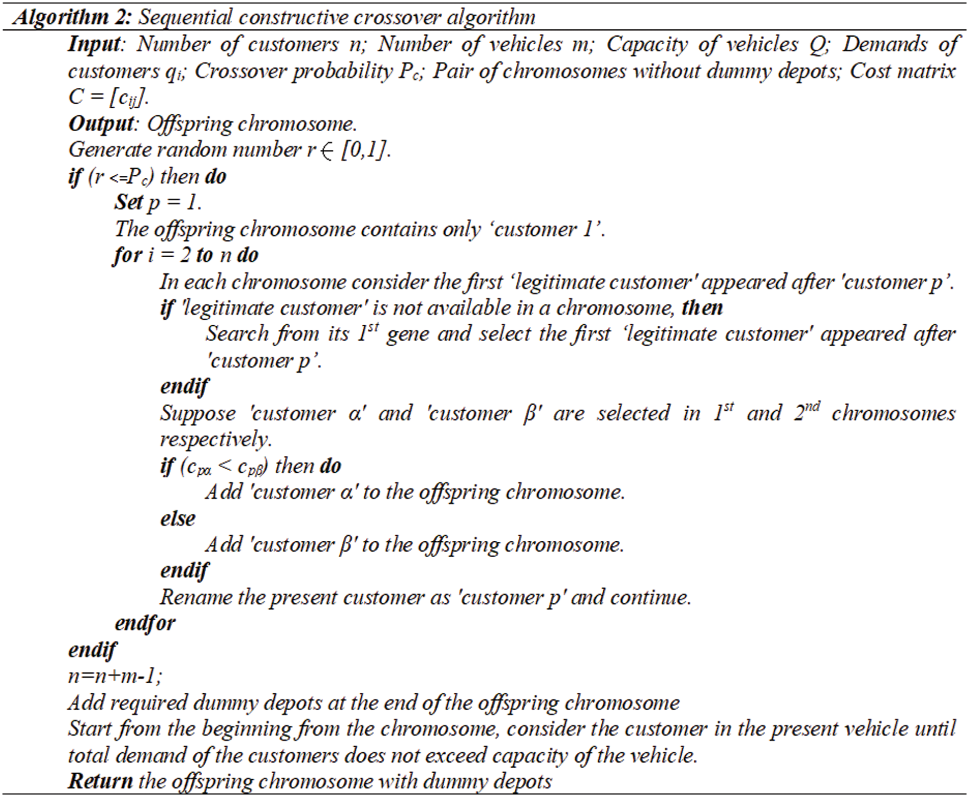
In [25], the SCX operator is proposed that creates only one offspring. It sequentially investigates parents and considers 1st legitimate gene (i.e., unvisited gene) that is found after the current gene in each parent. If no legitimate gene is discovered in a parent, it sequentially investigates from the starting of the parent and choose the legitimate gene. It then evaluates the cost of each gene and add the better one to the offspring. Algorithm 2 reports the algorithm for the SCX.

Consider the same example parent chromosomes P1: (1, 6, 9, 8, 5, 3, 2, 4, 7) and P2: (1, 8, 6, 9, 4, 3, 7, 5, 2).

Initially, the offspring is (1). The legitimate customers after customer 1 in the parents are 6 and 8 with their costs 17 and 9 respectively. Since customer 8 is cheaper, we add it to the offspring that leads to: (1, 8).

The legitimate customers after customer 8 in the parents are 5 and 6 with their costs 13 and 9 respectively. Since customer 6 is cheaper, we add it to the offspring that leads to: (1, 8, 6).

Since the legitimate customer after customer 6 in the parents are same 9, we add it to the offspring that leads to: (1, 8, 6, 9).

The legitimate customers after customer 9 in the parents are 5 and 4 with their costs 9 and 14 respectively. Since customer 5 is cheaper, we add it to the offspring that leads to: (1, 8, 6, 9, 5).

The legitimate customers after customer 5 in the parents are 3 and 2 with their costs 21 and 15 respectively. Since customer 2 is cheaper, we add it to the offspring that leads to: (1, 8, 6, 9, 5, 2). This way, we create the complete offspring as: (1, 8, 6, 9, 5, 2, 4, 7, 3).

Next, we add dummy depots at the end of the offspring chromosome which becomes: O: (1, 8, 6, 9, 5, 2, 4, 7, 3, 10). Then calculate total demand of the customers. So, we have, (q1 + q8 + q6 + q9 + q5) = 0 + 18 + 25 + 12 + 27 = 82. Now if we add q2 = 24, then 82 + 24 = 106 > 100 (=Q), hence, we exchange ‘customer 2’ with ‘customer 10’. So, the offspring becomes O: (1, 8, 6, 9, 5, 10, 4, 7, 3, 2) with cost 139.

Amongst the above eight crossovers GX, HX, MHX and SCX are the distance-based crossovers, and OX, PMX, CX and AEX are the blind crossovers. We propose to compare both categories of crossovers for the CVRP.

4.4 Mutation Operator

To diversify the population, mutation operator is applied with a prespecified probability. Generally, mutation probability is set very low compared to crossover probability. The exchange mutation that chooses randomly two places in a chromosome within a route of any vehicle and exchanges their values. If there are m vehicles, there will be m exchanges. This mutation will always produce legal chromosome. For example, let the Chromosome: (1, 8, 6, 2, 3, 4, 10, 7, 9, 5) with cost 143 is allowed for the mutation. Suppose 5th and 6th position values (route of first vehicle), and 8th and 9th position values (route of second vehicle) in the chromosome are swapped. Then the muted chromosome will be Muted: (1, 8, 6, 2, 4, 3, 10, 9, 7, 5) with cost 138. However, we do not see whether the value of muted chromosome is better than the original chromosome.

4.5 Design of GAs

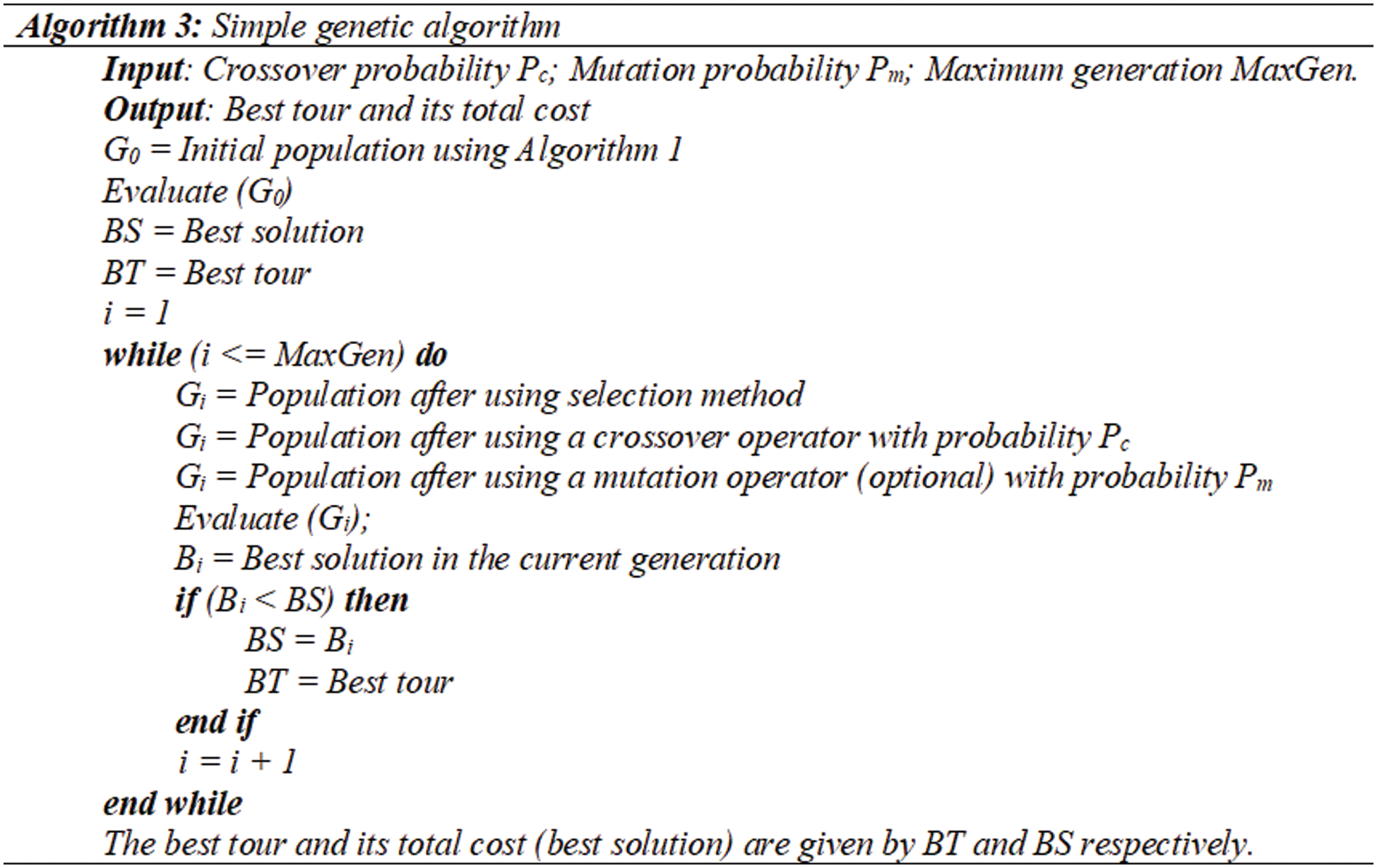
Our simple GA for the CVRP is presented in Algorithm 3.

We consider four blind crossovers and four distance-based crossovers. In each crossover selection, a single crossover is used. For mutation, two possibilities of selection–absence or presence of mutation, are applied. So, there are eight choices for crossover and two choices of mutation, thus provides sixteen variations of GAs. The aim of such individual implementation is to evaluate usefulness of the crossovers and to find their relative ranking. Notice that each GA is solely simple, not hybrid, that is developed of GA processes and basic operators, is not merging any other algorithm.

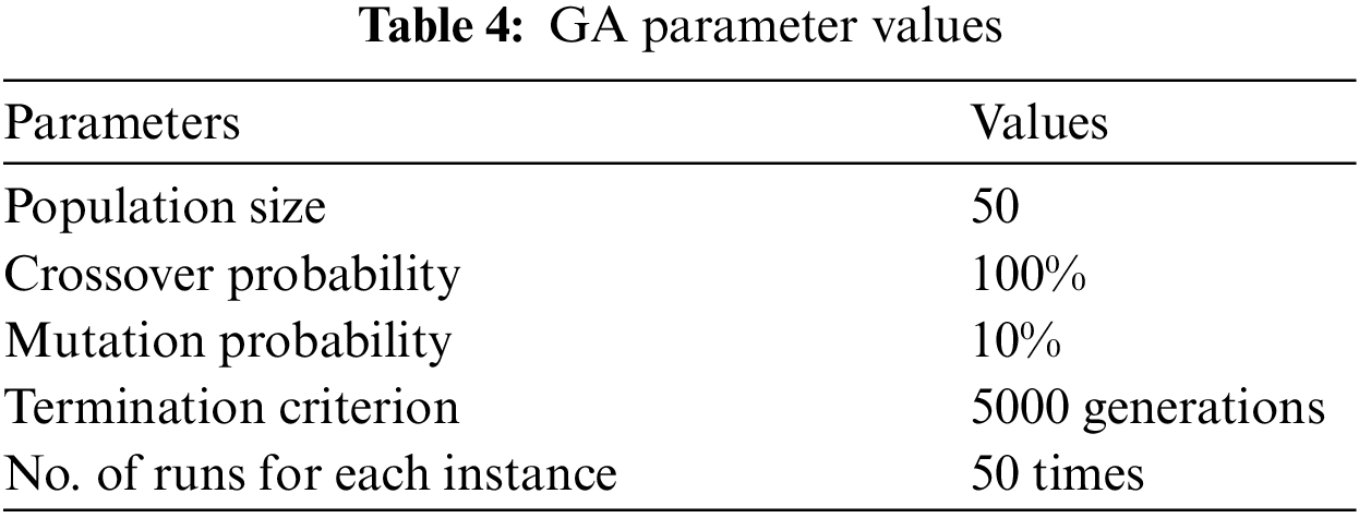
Basically, GA process is led by some GA parameters, specifically, population size which fixes number of chromosomes in every population, crossover probability for executing crossover between the parents, mutation probability for performing mutation operation, and a stopping criterion to end the GA process.

5  Computational Results

For comparing the effectiveness of various crossovers, simple GAs using various crossovers were encoded in Visual C++ on a Laptop with i7-1065G7 CPU@1.30 GHz and 8 GB RAM under MS Windows 10. We executed our GAs using various parameter sets, and finally, the parameters showed in Tab. 4 are chosen.

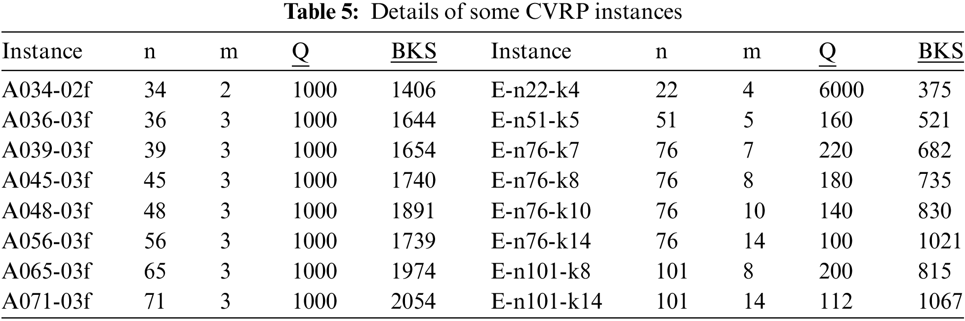
To verify the performance of crossovers, computational experiment is made on sixteen benchmark instances of many sizes. In these sixteen instances, A034-02f, A036-03f, A039-03f, A045-03f, A048-03f, A056-03f, A065-03f and A071-03f are asymmetric [35] , and E-n22-k4, E-n51-k5, E-n76-k7, E-n76-k8, E-n76-k10, E-n76-k14, E-n101-k8 and E-n101-k14 are symmetric [36]. The details of these sixteen problem instances are given in Tab. 5, where n is the number of customers (including depot), m is the number of vehicles, Q is the capacity of the vehicles, and BKS is the best-known/optimal solution.

The experimental results by the sixteen GAs are summarized in Tabs. 6, 8, 10 and 12. All these tables are structured in the same way: each row is for an instance (its optimal or best-known solution is written within brackets) and each column is for a simple GA using one crossover. So, a table element reports brief results of subsequent instance by subsequent GA. Each result is defined using best solution, average solution, average percentage of excess to the best-known solution, standard deviation (SD) of solutions, and average computational time (in second). For each instance, the best result over all GAs is indicated by boldface. The percentage of excess to the best-known solution, stated in various literatures, is calculated by following formula.

Excess(%)=Sol.Obtained−Best−KnownSol.BestKnownSolx100(5)

Figs. 3 and 4 show results for the asymmetric instance A071-03f (considering only 100 generations). Fig. 3 is for the GAs without mutation operator, and Fig. 4 is for the GAs with mutation operator. In these figures, each graph relates to one crossover that indicates how the solution improves in consecutive generations. In these figures, label on left side denotes the percentage of excess to the best-known solution (Excess (%)). When seeking to combine an allele in chromosome, all crossovers have some arbitrary factors that can make them further efficient.

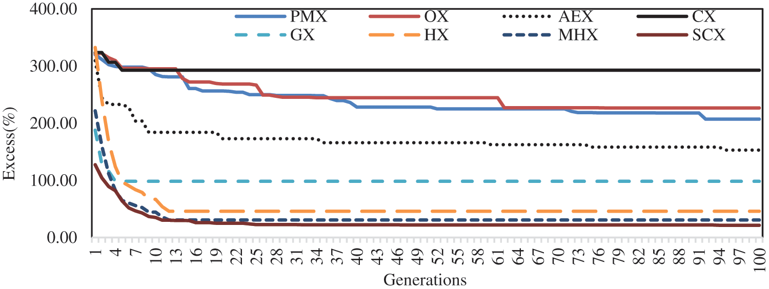
Figure 3: Performance of eight crossover operators without mutation for the instance A071-03f

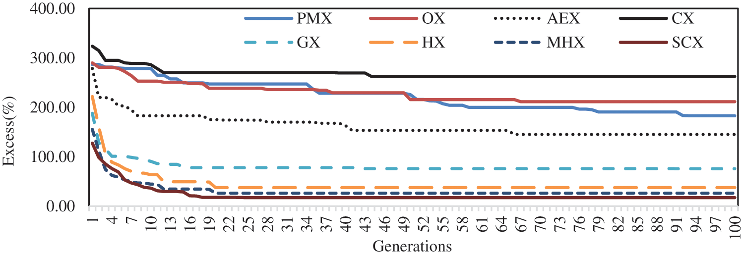
Figure 4: Performance of eight crossover operators with mutation for the instance A071-03f

Fig. 3 shows that among blind-crossovers, CX has initial variation within first 5 generations, after which it shows no variation, and so, it is found to be the worst one. Among remaining three blind-crossovers, the crossovers PMX and OX have shown good variation throughout the generations, however, they show slow improvement. The crossover AEX has shown very good variation within first 20 generations, after which it shows little variation and slow improvement. Of course, among the blind-crossovers, it is found to be the best one. The Figure also shows that among distance-based crossovers, GX has shown good initial variation within first 5 generations, after which it shows no variation, and so, it is found to be the worst among the distance-based crossover. The crossovers HX and MHX have shown good variation within first 15 generations, after which they show no variation. The figure for the crossover SCX shows that it starts the search process with better initial solutions, has shown good variation within first 25 generations, after which it shows no variation. Though SCX gets stuck in local minima after 25 generations, however, it is observed to be the best one among all crossover operators.

Fig. 4 shows that among blind-crossovers, PMX, OX and CX, each with mutation, have initial variations, and are competing within first 50 generations, after which CX shows no variation, but PMX and OX have small variations. So, CX is found to be the worst one. The crossover AEX shows very good variation within first 5 generations, has variation up to 67 generations, and is found to be best one among blind crossovers with mutation. Among distance-based crossovers with mutation, GX has initial variation within first 20 generations, after which it shows no variation. The remaining three distance-based crossovers have good variations within first 25 generations, and after that they are competing each other, and finally, SCX with mutation is observed to be best one among all crossovers. So, in both cases–with and without mutation, the crossover SCX is found to be the best one and CX is found to be the worst one. Further, it is seen that mutation operator enhances performance of crossovers by avoiding local minimum.

Tab. 6 describes the results on eight asymmetric instances by the eight GAs with no mutation operator. Based on the average solution and SD, the results are evaluated. With regard to the average solution, the distance-based crossovers are found much better than the blind crossovers. Among the blind crossovers, PMX and CX could not find lowest average solution for any of experimented eight instances. Between the crossovers PMX and CX, the crossover PMX is found to be better. So, the crossover CX is the worst one. The crossover OX obtained lowest solution for only one instance, A034-02f, and AEX obtained lowest solution for the remaining seven instances. So, amongst the blind crossovers, AEX is observed to be the best one and CX is the worst one. However, CX takes less time.

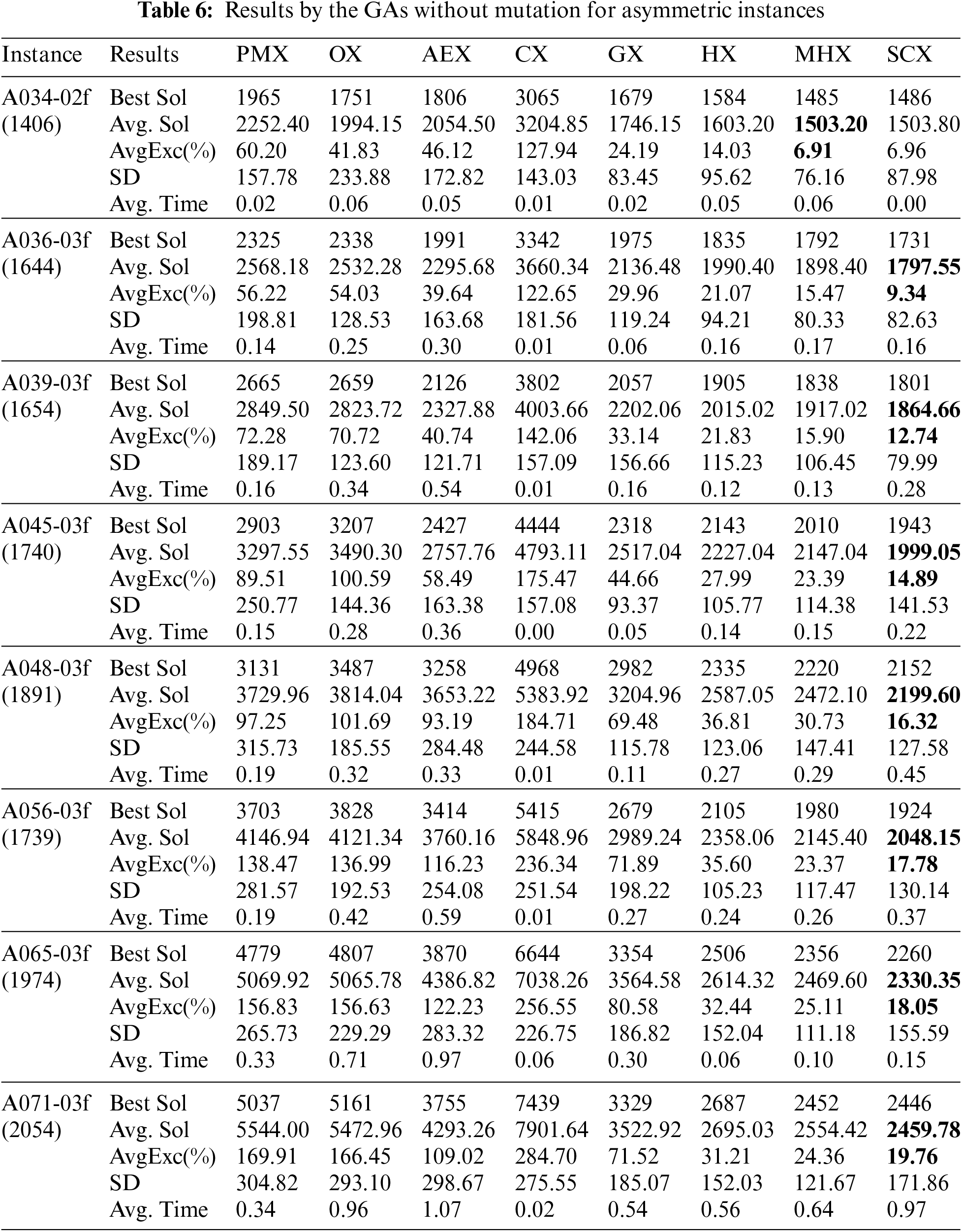
Amongst the distance-based crossovers, HX and GX could not find lowest average cost for any of experimented eight instances. Between GX and HX, HX is found better than GX. So, GX is observed to be the worst one among distance-based crossovers, yet GX is found better than AEX. The crossover MHX obtained lowest cost for only one instance, A034-02f, SCX obtained lowest cost for the remaining seven instances. So, among distance-based crossovers, SCX is observed to be best one. In fact, among all eight crossovers, SCX is observed to be best one. In addition, since the solutions obtained by SCX has lowest SD, one can conclude that the results by SCX is stable. Next, if one looks very carefully, then one can tell that MHX is the 2nd best and CX is the worst one. Further, the results of GX, HX, MHX and SCX are depicted in Fig. 5, which also confirms our conclusion.

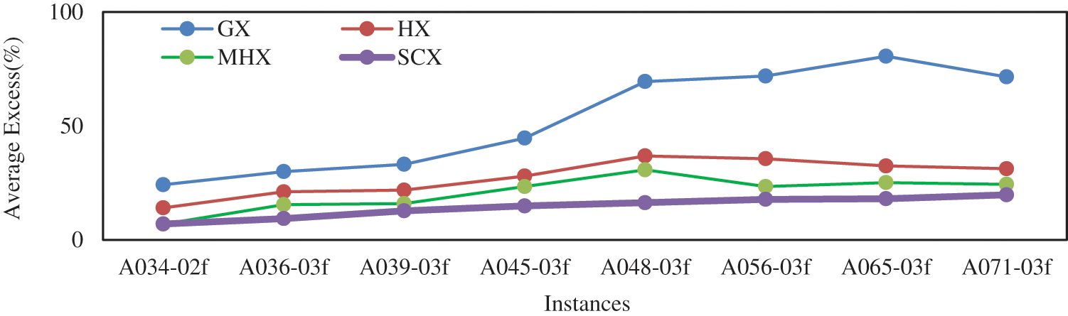
Figure 5: Average Excess (%) by GAs without mutation for asymmetric instances

To verify if GA using SCX (with no mutation) found much different average solution from the average solutions found by other GAs using distance-based crossovers, we conducted Student’s t-test. Further, we verify whether GA using AEX found much different average solution from the average solutions found by other GAs using blind crossovers. We applied following t-test formula for two large independent samples [37]. The values of X¯2 and SD2 are obtained by a GA using a particular crossover, while of X¯1 and SD1 values are obtained by its competing GAs.

t=X¯1−X¯2SD12n1−1+SD22n2−1

where,

X¯1−averageoffirstsample,

SD1−standarddeviationoffirstsample,

X¯2−averageofsecondsample,

SD2−standarddeviationofsecondsample,

n1−firstsamplesize,

n2−secondsamplesize,

Tab. 7 reports the t-statistic values that may be negative or positive. The positive value suggests that a particular crossover-based GA found better solution than its competing GA variant. If the value is negative, the competing algorithm found better solution. The confidence interval is applied at 95% confidence level (t0.05 = 1.96). If t-value is more than 1.96 and positive, the two values have much difference, and so, the GA using the particular crossover found better solution. If t-value is more than 1.96 and negative, the competing GA found better solution. If t-value is less than 1.96, and positive or negative, the algorithms could not find different solutions. The table further concludes about which crossover is better.

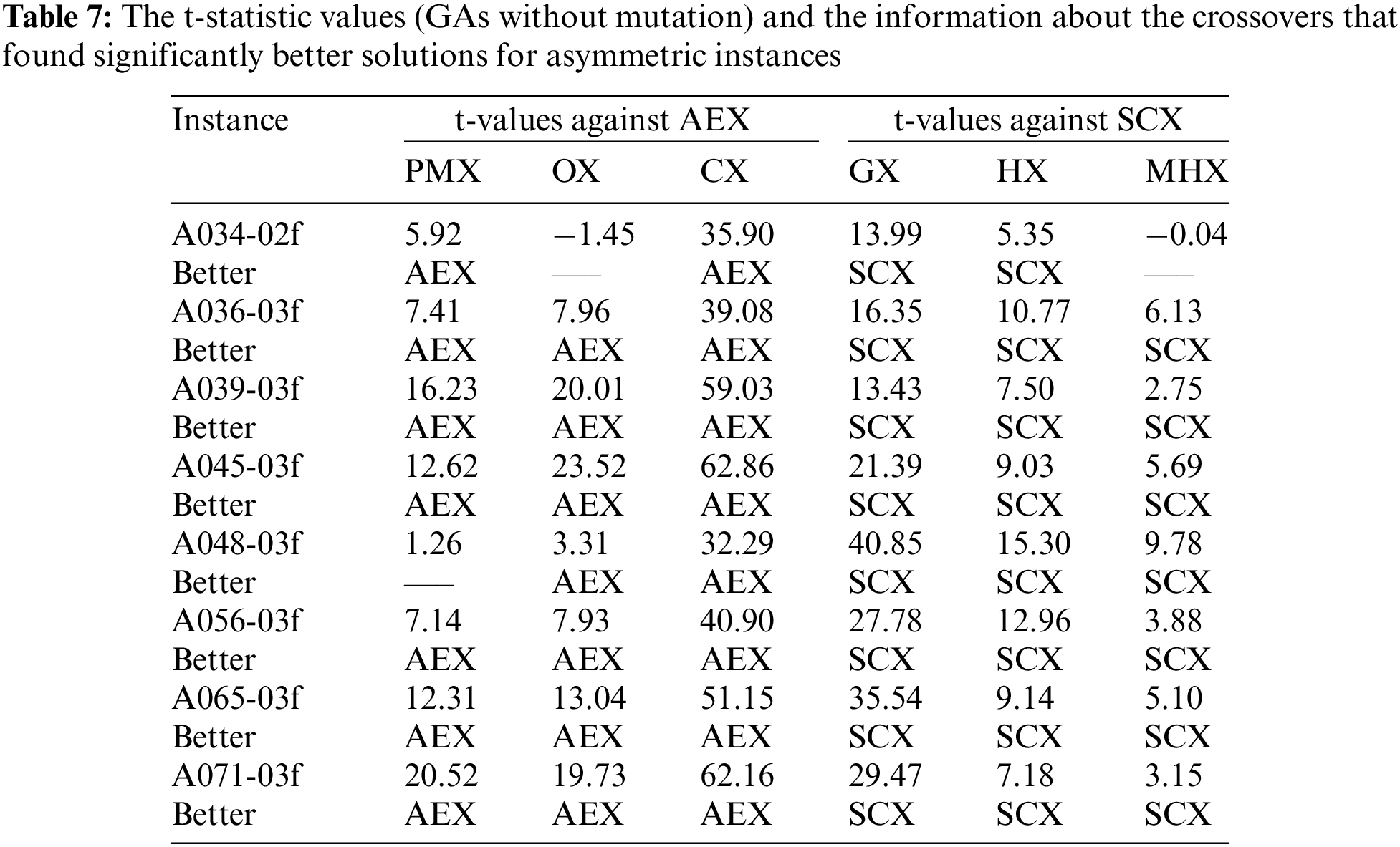
According to the results shown in Tab. 7, when comparing AEX against blind crossovers, we found that AEX is better than CX on all eight instances. Further, AEX is better than PMX and OX on seven instances and for only one instance, AEX and PMX have no difference, and AEX and OX have no difference. So, AEX is the best crossover and CX is the worst one among the blind crossover operators. About the distance-based crossovers, on all instances SCX is better than GX and HX. For one instance only, SCX and MHX have no difference, and SCX is better than MHX on the remaining seven instances. So, SCX is the best one and GX is the worst one among the distance-based crossovers. Further, SCX is compared with all other crossovers and found that SCX is the best one, however it is not reported.

Tab. 8 describes the results on asymmetric instances by all GAs using mutation. With respect to the average solution, it is very clear from Tab. 8 also that the distance-based crossovers are far better than the blind crossovers. Among the blind crossovers, PMX, OX and CX could not find lowest average solution for any of experimented eight instances. The crossover AEX obtained lowest solutions for all eight instances. So, among the blind crossovers, AEX is the best one and CX is the worst one for both GAs with and without mutation for these asymmetric instances. Among the distance-based crossovers, GX, HX and MHX could not find lowest average solution for any of experimented eight instances. SCX obtained lowest solutions for all instances, and hence it is the best. In addition, since the solutions obtained by SCX has lowest SD, one can conclude that the results by SCX is stable. Though GX is the worst among the distance-based crossovers, however, it is better than AEX for both GAs with and without mutation operator. The results of GX, HX, MHX and SCX are further displayed in Fig. 6, which shows that SCX is the best one, MHX is better than HX, and HX is better than GX.

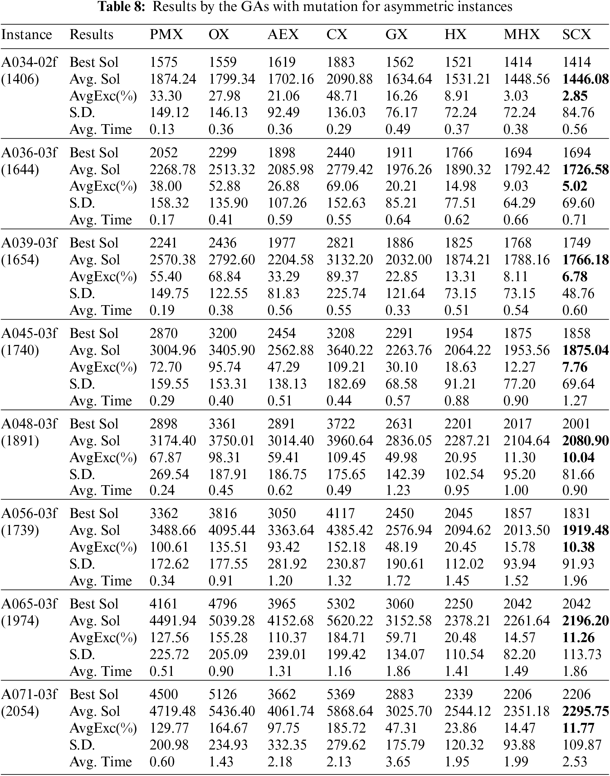
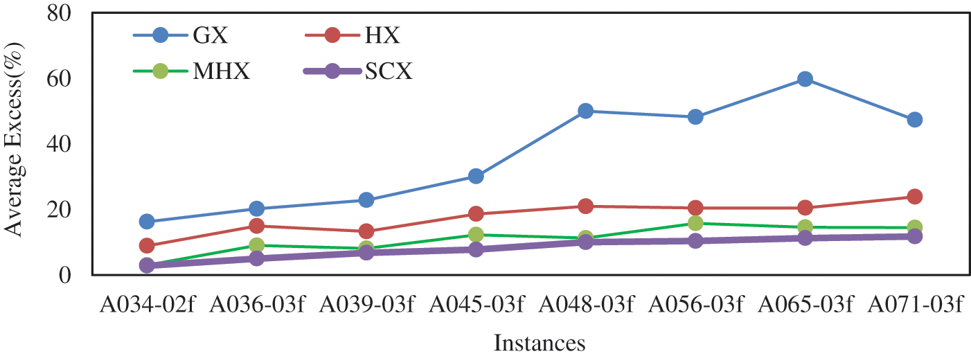
Figure 6: Average Excess (%) by GAs with mutation for asymmetric instances

Further, to verify if GA using SCX (including mutation) found much different average solution from the average solutions found by other GAs using distance-based crossovers, we conducted Student’s t-test. Further, we verify whether GA using AEX found much different average solution from the average solutions found by other GAs using blind crossovers. The t-statistic values are reported in the Tab. 9.

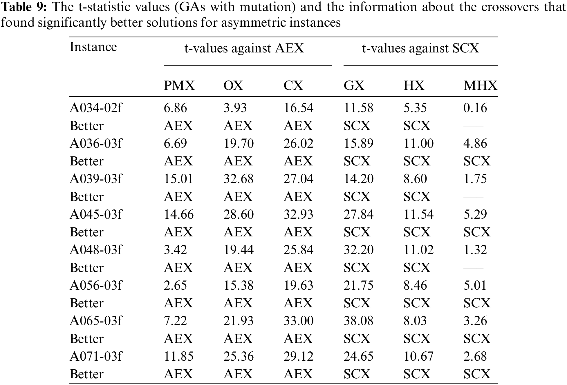
According to the results shown in Tab. 9, when comparing AEX against other blind crossovers, we observed that AEX is better than CX, OX and PMX on all eight instances. Also, we found that among CX, OX and PMX, the crossover CX is the worst one. So, AEX is the best crossover and CX is the worst one among the blind crossover operators for asymmetric instances. About the distance-based crossovers, on all eight instances SCX is better than GX and HX. For three instances only, SCX and MHX have no difference, and SCX is better than MHX on the remaining five instances. So, SCX is the best one and GX is the worst one among the distance-based crossovers. Further, SCX is compared with all other crossovers and found that SCX is the best one, however it is not reported.

We now extend our study on symmetric instances. Tab. 10 describes results on eight symmetric instances by the eight GAs without mutation. With regard to the average solution, for symmetric instances also the distance-based crossovers are much better than the blind crossovers. Amongst the blind crossovers, CX could not find lowest average solution for a single instance. The crossovers OX, PMX and AEX could find lowest average solution for one, three and four instances respectively. So, among the blind crossovers, AEX is found to be the best one and CX is the worst one. Amongst the distance-based crossovers, GX and HX could not find lowest average solution for a single symmetric instance. However, between GX and HX, HX is better than GX, and GX is better than AEX. The crossovers MHX and SCX could find lowest solution for three and five instances respectively. Among the distance-based crossovers, though MHX and SCX are competing, still SCX is found to be the best one. Among all crossovers, SCX is the best one and CX is the worst one. The results of GX, HX, MHX and SCX are also displayed in Fig. 7 that verifies our conclusion.

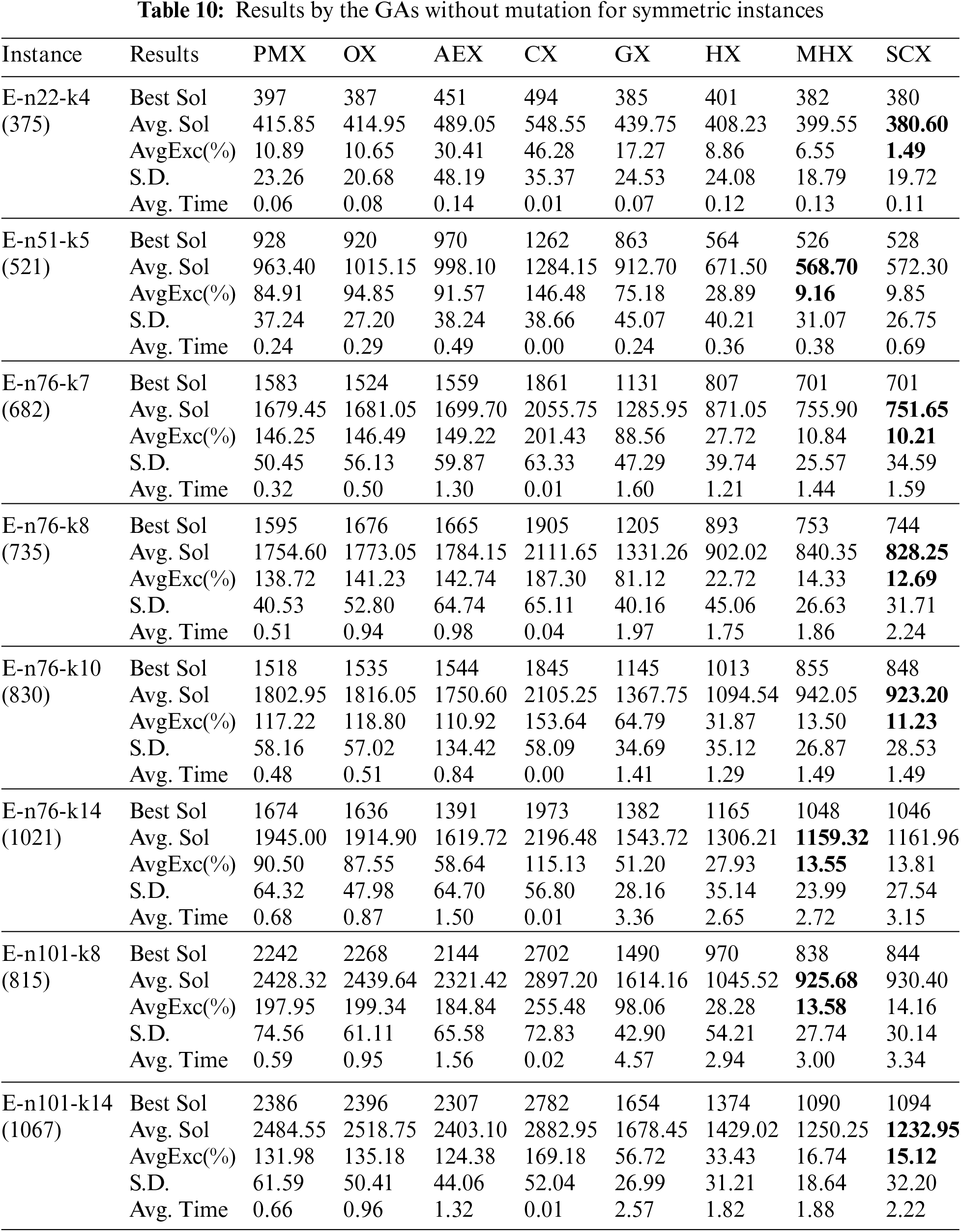
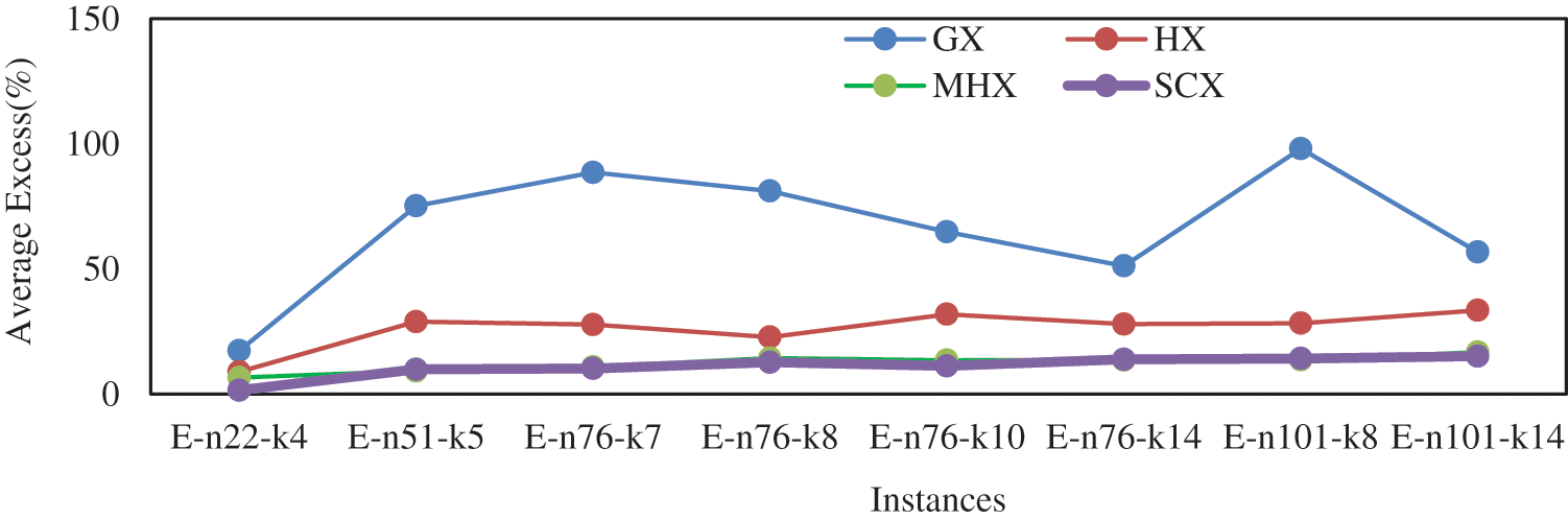
Figure 7: Average Excess (%) by GAs without mutation for symmetric instances

Further, to verify if GA using SCX (excluding mutation) found much different average solution from the average solutions found by other GAs using the distance-based crossovers, we conducted Student’s t-test. Further, we verify whether GA using AEX found much different average solution from the average solutions found by other GAs using the blind crossovers. The t-statistic values are reported in the Tab. 11.

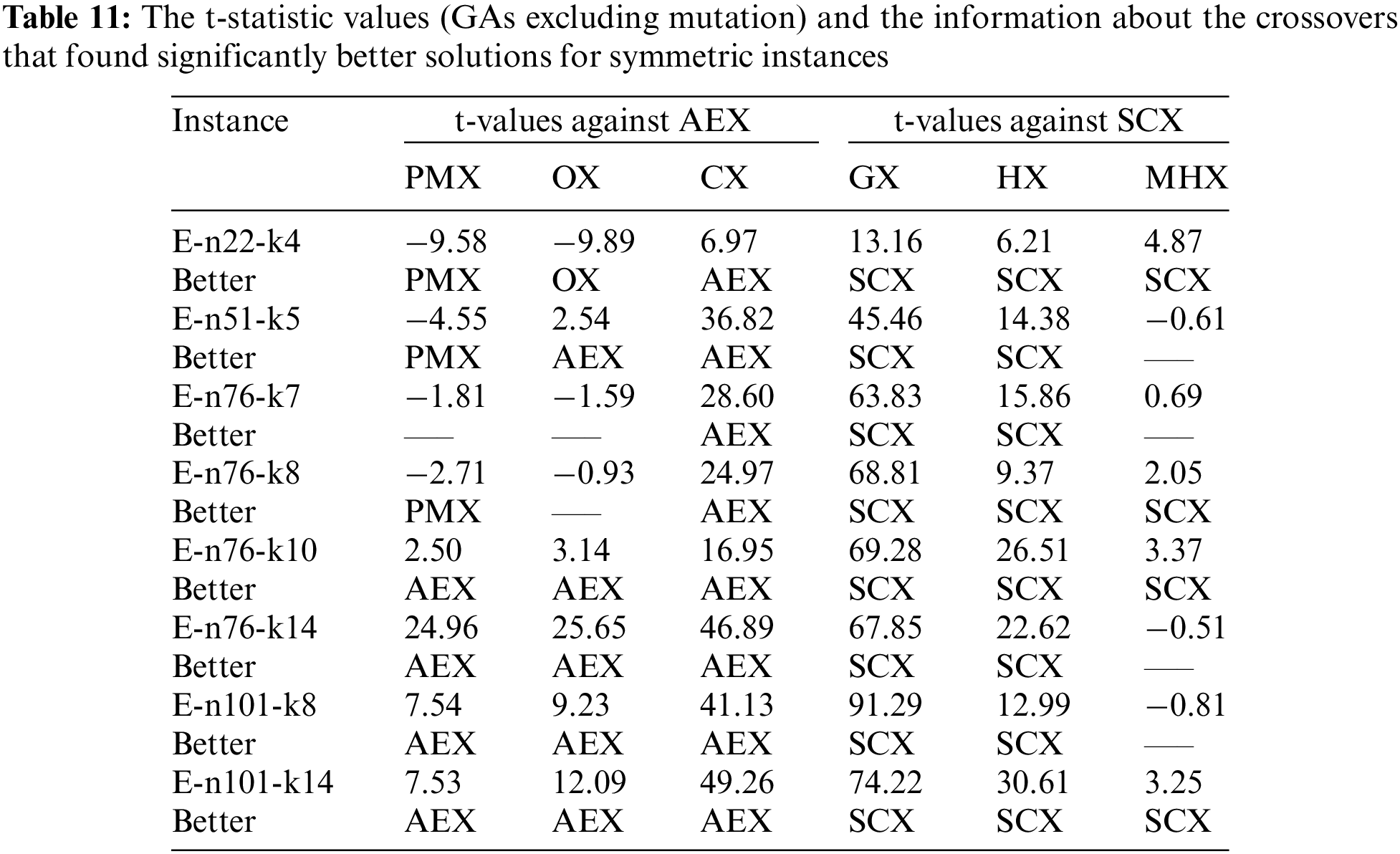
According to Tab. 11, for a single instance, AEX and PMX have no difference. For three instances PMX is better than AEX, and for four instances AEX is better than PMX. So, AEX is better than PMX. For two instances, AEX and OX have no difference. For a single instance, OX is better than AEX, and for five instances AEX is better than OX. So, AEX is better than OX. For all instances, AEX is better than CX. So, AEX is the best crossover and CX is the worst one among the blind crossover operators for symmetric instances. About the distance-based crossovers, on all eight symmetric instances SCX is better than GX and HX. However, between GX and HX, HX is better than GX. For four instances, SCX and MHX have no difference, and SCX is better than MHX on the remaining four instances. So, SCX is the best one and GX is the worst one among the distance-based crossovers for symmetric instances.

We now continue our study of the GAs with mutation on symmetric instances, and Tab. 12 describes results on eight symmetric instances. With regard to the average solution, for symmetric instances also the distance-based crossovers with mutation are much better than the blind crossovers with mutation. Among the blind crossovers, OX and CX could not find lowest average solution for any of the eight instances. Between these two crossovers, OX is found to be better than CX. The crossovers PMX and AEX could find lowest average solution for four instances each. So, among the blind crossovers PMX and AEX, each with mutation, are competing. Among the distance-based crossovers, GX and HX, each with mutation, could not find lowest average solution for any of the eight symmetric instances. However, GX is better than PMX and AEX, and HX is found to be better than GX. The crossovers MHX and SCX, each with mutation, could find lowest cost for one and seven instances respectively. So, among the distance-based crossovers, SCX with mutation is the best crossover and GX with mutation is the worst one. So, among all crossovers, SCX with mutation is the best one and CX is the worst one. The results of GX, HX, MHX and SCX are also depicted in Fig. 8 that verifies our conclusion.

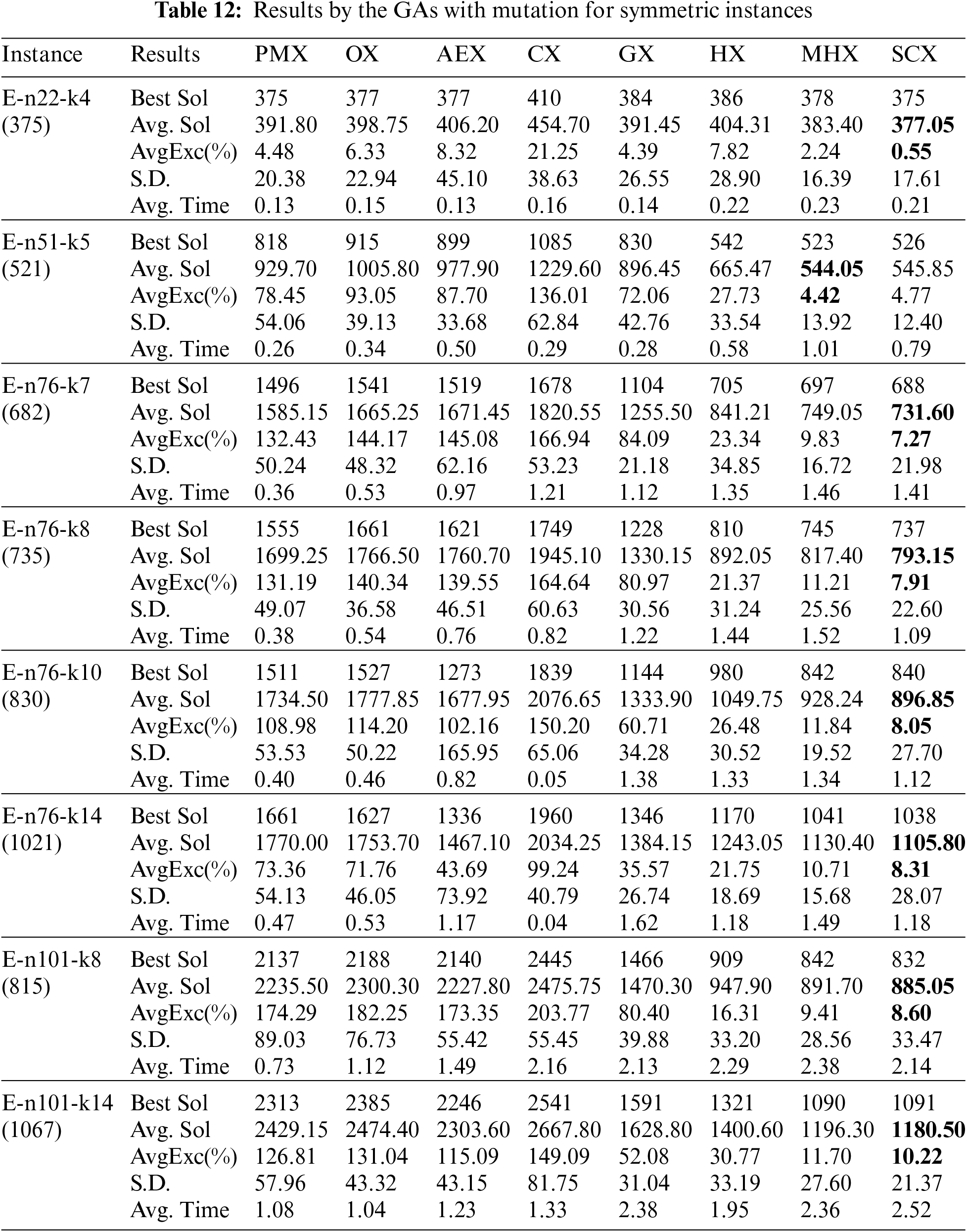
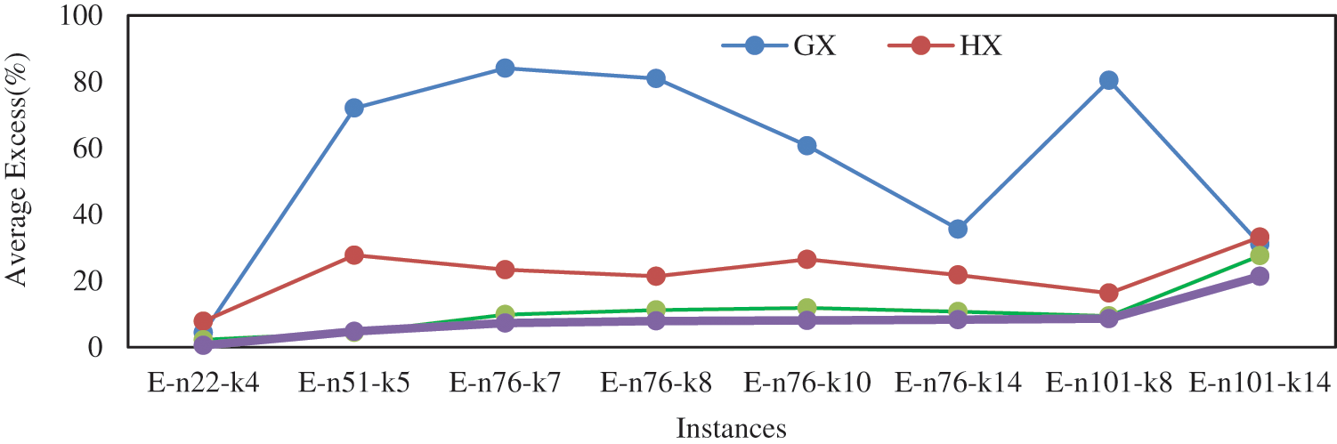
Figure 8: Average Excess (%) by GAs with mutation for asymmetric instances

Further, to verify if GA using SCX (including mutation) found much different average solution from the average solutions found by other GAs using the distance-based crossovers and mutation for symmetric instances, we conducted Student’s t-test. Further, we verify whether GA using AEX found much different average solution from the average solutions found by other GAs using the blind crossovers and mutation. The t-statistic values are reported in the Tab. 13.

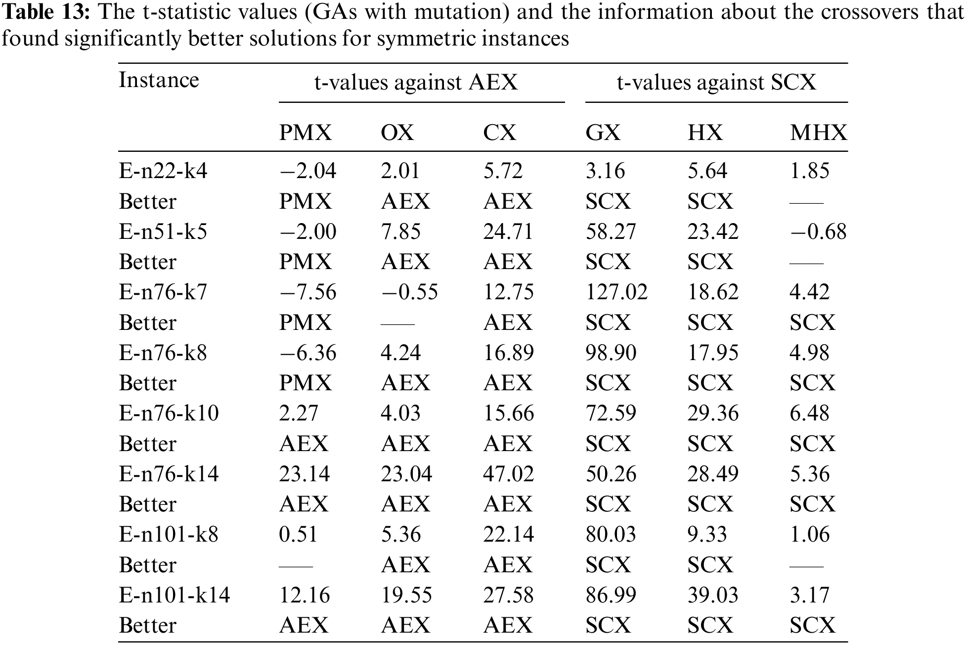
According to Tab. 13, for a single instance, AEX and PMX have no difference. For three instances AEX is better than PMX, and for four instances PMX is better than AEX. So, PMX is better than AEX. For a single instance, AEX and OX have no difference. On the remaining seven instances, AEX is better than OX. So, AEX is better than OX. On all eight instances, AEX is better than CX. So, PMX with mutation is the best one and CX with mutation is the worst one among the blind crossovers. About distance-based crossovers, on all eight symmetric instances SCX is better than GX and HX. For seven instances, HX is better than GX. For three symmetric instances SCX and MHX have no difference, and for other five instances SCX is better than MHX. For all instances, MHX is better than HX. So, SCX with mutation is the best one and GX with mutation is the worst one among the distance-based crossovers for symmetric instances.

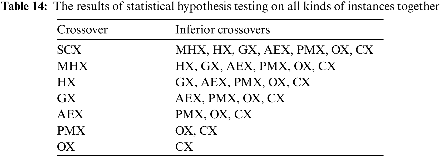
Overall, SCX is the best and MHX is the second best, and CX is the worst for the CVRP. To make a ranking of the crossovers, we conducted a series of Student’s t-tests on all kinds of instances together. In fact, for each pair of crossovers, we tested the hypothesis to know which one is better. We summarized the results in Tab. 14, where every row has two columns-1st column is for crossover(s) and 2nd one is for its inferior crossovers. It is observed that there is significant statistical difference between SCX and other crossovers, and so, as estimated, the best crossover is SCX, the 2nd best is MHX, and the worst is CX. The crossover SCX conserves the merits of parents and tries to reduce the local cost between the adjacent customers in the offspring chromosomes by sequentially scan the parent chromosomes. However, other crossovers could not reduce local costs between adjacent customers.

6  Conclusion and Future Works

In this research we studied the capacitated vehicle routing problem (CVRP) that is a mixture of the travelling salesman problem (TSP) and the bin packing problem (BPP). A number of crossovers in genetic algorithms (GAs) were suggested for the TSP that can be utilized for the CVRP. Selecting efficient crossover may lead to efficient GA. We developed eight GAs using four blind crossovers-partially mapped crossover (PMX), order crossover (OX), alternating edges crossover (AEX), and cycle crossover (CX), and four distance-based crossovers-heuristic crossover (HX), greedy crossover (GX), modified heuristic crossover (MHX) and sequential constructive crossover (SCX) without mutation, and another eight GAs using above eight crossovers with mutation operator. First, the crossovers were illustrated using same parent chromosomes for building offspring(s), and then all GAs were coded in Visual C++. The usefulness of the crossovers is determined by solving some asymmetric and symmetric instances of numerous sizes. The investigational results reveal the usefulness of AEX among the blind crossovers, and SCX among the distance-based crossovers for the CVRP. So, our study revealed that the distance-based crossovers are much superior to the blind crossovers. Further, we observed that the best crossover is SCX, the 2nd best is MHX, and the worst is CX. This estimation is validated by Student’s t-test at 95% confidence level. If only a single crossover operator is applied, then, whether mutation is applied or not, the best performance is accomplished SCX. Exceptionally bad performance is shown by CX, if mutation is present or not.

There are many crossover operators present in the literature, but all of them may not provide legal solution to the CVRP. Therefore, this paper is confined to study few crossover operators. We aimed to compare amongst eight crossovers without and with a mutation operator. Our aim was not to develop efficient GA. We did not apply either a local search method or merge some heuristics to enhance the solution value to obtain optimal solution. We restricted ourselves to design only simple GAs. Further, the highest crossover probability is set to present exact character of crossovers. Though SCX obtained very good results, still it got stuck in local minima in the initial generations. Hence, successful local search and immigration procedures might be merged to hybridize the GA for obtaining improved results to various instances, which is our next research.

Data Availability: e data set used to support the findings of this study is available from the corresponding author upon request.

Funding Statement: The authors are very much thankful to the anonymous honorable reviewers for their careful reading of the paper and their many insightful comments and constructive suggestions which helped the authors to improve the paper. The authors extend their appreciation to the Deanship of Scientific Research at Imam Mohammad Ibn Saud Islamic University for funding this work through Research Group No. RG-21-09-17.

Conflicts of Interest: The authors declare that they have no conflicts of interest to report regarding the present study.

References

1. G. B. Dantzig and J. H. Ramser, “The truck dispatching problem,” Management Science, vol. 6, no. 1, pp. 80–91, 1959. [Google Scholar]
2. F. Daneshzand, “The vehicle-routing problem,” Logistics Operations and Management, vol. 8, pp. 127–153, 2011. [Google Scholar]
3. Y. Yao, Y. Zhang, L. Tian, N. Zhou, Z. Li et al., “Analysis of network structure of urban bike-sharing system: A case study based on real-time data of a public bicycle system,” Sustainability, vol. 11, no. 19, pp. 1–17, 2019. [Google Scholar]
4. M. A. Rahman, A. -A. Hossain, B. Debnath, Z. M. Zefat, M. S. Morshed et al., “Intelligent vehicle scheduling and routing for a chain of retail stores: A case study of Dhaka, Bangladesh,” Logistics, vol. 5, no. 3, pp. 1–20, 2021. [Google Scholar]
5. S. I. Khan, Z. Qadir, H. S. Munawar, S. R. Nayak, A. K. Budati et al., “UAVs path planning architecture for effective medical emergency response in future networks,” Physical Communication, vol. 47, 101337, 2021. [Google Scholar]
6. P. Toth and D.Vigo, “Vehicle routing: Problems, methods, and applications,” P. Toth and D. Vigo, (Eds.Society for Industrial and Applied Mathematics, Philadelphia, PA, USA, pp. 1–33, 2014. [Google Scholar]
7. J. D. E. Little, K. G. Murthy, D. W. Sweeny and C. Karel, “An algorithm for the travelling salesman problem,” Operations Research, vol. 11, pp. 972–989, 1963. [Google Scholar]
8. C. Barnhart, E. L. Johnson, G. L. Nemhauser, M. W. Savelsbergh and P. H. Vance, “Branch-and-price: Column generation for solving huge integer programs,” Operations Research, vol. 46, no. 3, pp. 316–329, 1998. [Google Scholar]
9. R. E. Gomory, “Outline of an algorithm for integer solutions to linear programs and an algorithm for the mixed integer problem,” in 50 Years of Integer Programming 1958–2008, Berlin, Heidelberg: Springer, pp. 77–103, 2010. [Google Scholar]
10. Z. H. Ahmed, “A Data-guided lexisearch algorithm for the asymmetric traveling salesman problem,” Mathematical Problems in Engineering, vol. 2011, Article ID 750968, pp. 1–18, 2011. [Google Scholar]
11. R. Tavakkoli-Moghaddam, N. Safaei and Y. Gholipour, “A hybrid simulated annealing for capacitated vehicle routing problems with the independent route length,” Applied Mathematics and Computation, vol. 176, no. 2, pp. 445–454, 2006. [Google Scholar]
12. M. -C. Bolduc, G. Laporte, J. Renaud and F. F. Boctor, “A tabu search heuristic for the split delivery vehicle routing problem with production and demand calendars,” European Journal of Operational Research, vol. 202, no. 1, pp. 122–130, 2010. [Google Scholar]
13. G. Fuellerer, K. F. Doerner, R. F. Hartl and M. Iori, “Ant colony optimization for the two-dimensional loading vehicle routing problem,” Computers and Operations Research, vol. 36, no. 3, pp. 655–673, 2009. [Google Scholar]
14. T. J. Ali and V. Kachitvichyanukul, “A particle swarm optimization for the vehicle routing problem with simultaneous pickup and delivery,” Computers and Operations Research, vol. 36, no. 5, pp. 1693–1702, 2009. [Google Scholar]
15. G. Jeon, H. O. Leep and J. Y. Shim, “A vehicle routing problem solved by using a hybrid genetic algorithm,” Computers and Industrial Engineering, vol. 53, no. 4, pp. 680–692, 2007. [Google Scholar]
16. N. Mladenovic, D. Urosevic, S. Hanafi and A. Ilic, “A general variable neighborhood search for the one-commodity pickup-and-delivery travelling salesman problem,” European Journal of Operational Research, vol. 220, no. 1, pp. 270–285, 2012. [Google Scholar]
17. D. E. Goldberg, Genetic Algorithms in Search, Optimization, and Machine Learning, 1st ed., New York: Addison-Wesley Longman Publishing Co., 1989. [Google Scholar]
18. C. Prins, “A simple and effective evolutionary algorithm for the vehicle routing problem,” Computers and Operations Research, vol. 31, no. 12, pp. 1985–2002, 2004. [Google Scholar]
19. M. Haj-Rachid, W. Ramdane-Cherif, P. Chatonnay and C. Bloch, “Comparing the performance of genetic operators for the vehicle routing problem,” IFAC Proceedings Volumes, vol. 43, no. 17, pp. 313–319, 2010. [Google Scholar]
20. N. Christophides and S. Eilon, “An algorithm for the vehicle despatching problem,” Operational Research Quaterly, vol. 20, no. 3, pp. 309–318, 1969. [Google Scholar]
21. H. Nazif and L. S. Lee, “Optimised crossover genetic algorithm for capacitated vehicle routing problem,” Applied Mathematical Modelling, vol. 36, no. 5, pp. 2110–2117, 2012. [Google Scholar]
22. K. Puljic and R. Manger, “Comparison of eight evolutionary crossover operators for the vehicle routing problem,” Journal of Mathematical Communications, vol. 18, no. 2, pp. 359–375, 2013. [Google Scholar]
23. S. G. V. Kumar and R. Panneerselvam, “A study of crossover operators for genetic algorithms to solve vrp and its variants and new sinusoidal motion crossover operator,” International Journal of Computational Intelligence Research, vol. 13, no. 7, pp. 1717–1733, 2017. [Google Scholar]
24. M. Sajid, J. Singh, R. A. Haidri, M. Prasad, V. Varadarajan et al., “A novel algorithm for capacitated vehicle routing problem for smart cities,” Symmetry, vol. 13, no. 10, pp. 1–23, 2021. [Google Scholar]
25. Z. H. Ahmed, “Genetic algorithm for the traveling salesman problem using sequential constructive crossover operator,” International Journal of Biometrics & Bioinformatics, vol. 3, no. 6, pp. 96–105, 2010. [Google Scholar]
26. E. Osaba, R. Carballedo, F. Diaz, E. Onieva, A. D. Masegosa et al., “Good practice proposal for the implementation, presentation, and comparison of metaheuristics for solving routing problems,” Neurocomputing, vol. 271, no. 3, pp. 2–8, 2018. [Google Scholar]
27. J. K. Lenstra and A. H. G. Rinnooy Kan, “Some simple applications of the travelling salesman problem,” Operational Research Quarterly, vol. 26, no. 4, pp. 717–733, 1975. [Google Scholar]
28. Z. H. Ahmed, “A lexisearch algorithm for the distance-constrained vehicle routing problem,” International Journal of Mathematical and Computational Methods, vol. 1, pp. 165–174, 2016. [Google Scholar]
29. D. E. Goldberg and R. Lingle, “Alleles, loci and the travelling salesman problem,” in Proc. ICGA, Pittsburgh, PA, USA, pp. 154–159, 1985. [Google Scholar]
30. L. Davis, “Job-shop scheduling with genetic algorithms,” in Proc. ICGA, Pittsburgh, PA, USA, pp. 136–140, 1985. [Google Scholar]
31. J. Grefenstette, R. Gopal, B. Rosmaita and D. Gucht, “Genetic algorithms for the traveling salesman problem,” in Proc. ICGA, Pittsburgh, PA, USA, pp. 160–168, 1985. [Google Scholar]
32. I. M. Oliver, D. J. Smith and J. R. C. Holland, “A study of permutation crossover operators on the travelling salesman problem,” in Proc. ICGA, MIT, Cambridge, MA, pp. 224–230, 1987. [Google Scholar]
33. J. J. Grefenstette, “Incorporating problem specific knowledge into genetic algorithms,” in Genetic Algorithms and Simulated Annealing, ed., Los Altos, CA: Morgan Kaufmann, pp. 42–57, 1987. [Google Scholar]
34. P. Jog, J. Y. Suh and D. Van Gucht, “The effects of population size, heuristic crossover and local improvement on a genetic algorithm for the traveling salesman problem,” in Proc. ICGA, Morgan Kaufmann Publishers, San Francisco, CA, USA, pp. 110–115, 1989. [Google Scholar]
35. M. Fischetti, P. Toth and D. Vigo, “A Branch-and-bound algorithm for the capacitated vehicle routing problem on directed graphs,” Operations Research, vol. 42, no. 5, pp. 846–859, 1994. [Google Scholar]
36. N. Christofides and S. Eilon, “An algorithm for the vehicle routing dispatching problem,” Operations Research Quaterly, vol. 20, pp. 309–318, 1969. [Google Scholar]
37. Z. H. Ahmed, “Adaptive sequential constructive crossover operator in a genetic algorithm for solving the traveling salesman problem,” International Journal of Advanced Computer Science and Applications (IJACSA), vol. 11, no. 2, pp. 593–605, 2020. [Google Scholar]
Cite This Article
Copyright © 2023 The Author(s). Published by Tech Science Press.
This work is licensed under a Creative Commons Attribution 4.0 International License , which permits unrestricted use, distribution, and reproduction in any medium, provided the original work is properly cited.
Downloads
Citation Tools