Liver Ailment Prediction Using Random Forest Model

1  Introduction

The liver is an important organ that performs essential roles such as generating enzymes, eliminating exhausted tissues or cells, and handling leftover products [1]. An individual can live just for a few days if the liver is shut down. There is a capability in the liver to harvest new liver from healthy liver cells, that quite exists known as astonishing. Due to this capability, the liver can continue its function even though only 25% of the liver is healthy and active while the rest of it is removed or ailing [2]. It performs an important role in various body functions from blood clotting and protein creation to cholesterol, glucose (sugar), and iron metabolism, and eliminates poisons from the body [3,4]. Any failure in these functions or injured by chemicals, illness with a virus, or under attack due to own immune system, can be the purpose of crucial demolition to the body, and the liver will come to be so spoiled which can be the cause of death [3,5].

As indicated by World Gastroenterology Organization (WGO) and World Health Organization (WHO), 35 million people die due to prolonged syndromes, among these syndromes, liver infection is one of the reluctant diseases [6,7]. Moreover, 50 million adults also suffer from chronic liver diseases. From the recent information from WGO and WHO, it is observed that 25 million United State (US) occupant is affected due to chronic liver diseases. In the US, around about 25 percent of death happens due to chronic liver diseases [1], [8,9].

1.1 Foremost Reasons for Liver Disease

When the liver comes to be infected, it can ground extreme annihilation to our health. There can be various factors and ailments that can gullible motivation to liver harm [4,5], [10].

•   Alcohol: Thick alcohol drinking is the most extreme cause of liver harm. When, individual beverage liquor, the liver gets occupied from its different capacities and considerations generally on redesigning liquor into a more modest amount of toxic form.

•   Obesity: It is a fatty liver disease if an individual; has an extra amount of fat that slopes to gather close to the liver.

•   Diabetes: About 50 percent of liver diseases are caused due to diabetes, extending the level of persuading insulin impact in greasy liver infection.

1.2 Common Liver Syndrome

•   Hepatitis: An illness that is delivered due to a feast of the virus, because of excrement contamination or direct connection with the septic ridiculous liquids.

•   Liver Cancer: The threat of devouring liver malignant growth is greater for people having cirrhosis and other sorts of hepatitis.

•   Cirrhosis: It is the most extreme serious liver sickness that occurs once ordinary liver cells are traded by defacement tissue as chronic liver diseases.

In the recent era, people are stood up to the huge amount of information kept in a few associations like hospitals, universities, and banks which is the inspiration point to us for finding a path to acquire precise information from this huge data and utilize this, especially in healthcare organizations. Researchers’ expression moving errands in the healthcare associations to forecast any kind of disease for the early prediction and treatment from the huge amount of healthcare data. Nowadays, the utilization of Machine Learning (ML) and Data Mining (DM) develop rudimentary in medical care because of its methodologies for example clustering, classification, and association rule mining (ARM) to determine repetitive patterns for sickness identification on clinical information [6,11].

However, this study aims to travel around the Random Forest (RF) for liver syndromes prediction in its early stages. This study also presents the comparison of other ML techniques utilized in previous studies that include Forest by Penalizing Attributes (Forest-PA), K-nearest neighbor (KNN), Multilayer Perceptron (MLP), Naïve Bayes (NB), Credal Decision Tree (CDT), Composite Hypercube on Iterated Random Projection (CHIRP), Support Vector Machine (SVM), Average One Dependency Estimator (A1DE), and Decision Tree (J48). These classifiers are evaluated on the liver dataset taken from the UCI repository. For the assessment of each classifier, different evaluation measures are used including Root Relative Squared Error (RRSE), Root Mean Squared Error (RMSE), accuracy, Matthew’s Correlation Coefficient (MCC), precision, specificity, recall, F-measure, and G-measure.

1.3 The Contributions of This Research

•   We explore RF classifier to predict liver syndrome in its early stage.

•   We compare the results of RF with nine other ML classifiers including NB, CHIRP, CDT, MLP, A1DE, KNN, J48, SVM, and Forest-PA.

•   We performe several experiments on the liver disease dataset available on the open-source UCI ML repository.

•   For the strengthening of outcomes, evaluation is done using RRSE, RMSE, Accuracy, MCC, Recall, Specificity, Precision, F-measure, and G-measure.

Hereinafter, Section 2 covers the exploration procedure that involves further subsections of dataset depiction, execution evaluation measures, proposed solution, and survey of utilized methods. Section 3 contains the results and discussion, Section 4 presents the threats to validity and finally, Section 5 concluded the paper.

2  Methodology

This study focuses on the exploration of RF as well as the comparison of RF with some other ML classifiers due to its procedure of worth, individual secreted patterns, and delivering unique information [11]. ML is additionally realized as a rising revolution that has made reflective positioned modifications in the data land [8,12]. Including RF, other ML classifiers utilized in this research are NB, A1DE, MLP, KNN, CHIRP, SVM, CDT, Forest-PA, and J48. All the research is completed via the methodology shown in Fig. 1. For validation of the model, the authors employed 10 fold cross-validation (10-FCV) technique. The 10-FCV assessment is imposed on each classifier to evaluate its enactment.

Figure 1: Our research methodology

The 10-FCV splits the dataset into ten equivalent parts. In every iteration of 10-FCV, one subset of the dataset is used for testing, while the other subsets are used for training. It is a standard approach for valuation [13]. The dataset and performance evaluation measures are further discussed in Section 2.1 and 2.2 respectively, while the proposed solution is discussed in Section 2.3 and other classifiers are briefly deliberated in Section 2.4.

2.1 Dataset Description

In this research, all analyses are done on the liver dataset available at UCI Repository1 . This dataset comprises seven features. Among these seven features, five are the blood tests including mcv, alkphos, sgpt, sgot, and gammagt that are assumed to be penetrating the liver syndrome. The list of attributes along with value types and description is presented in Tab. 1 with normal value ranges. This dataset contains 345 instances of two types of selector that is either 1 or 2 which is shown in Fig. 2.

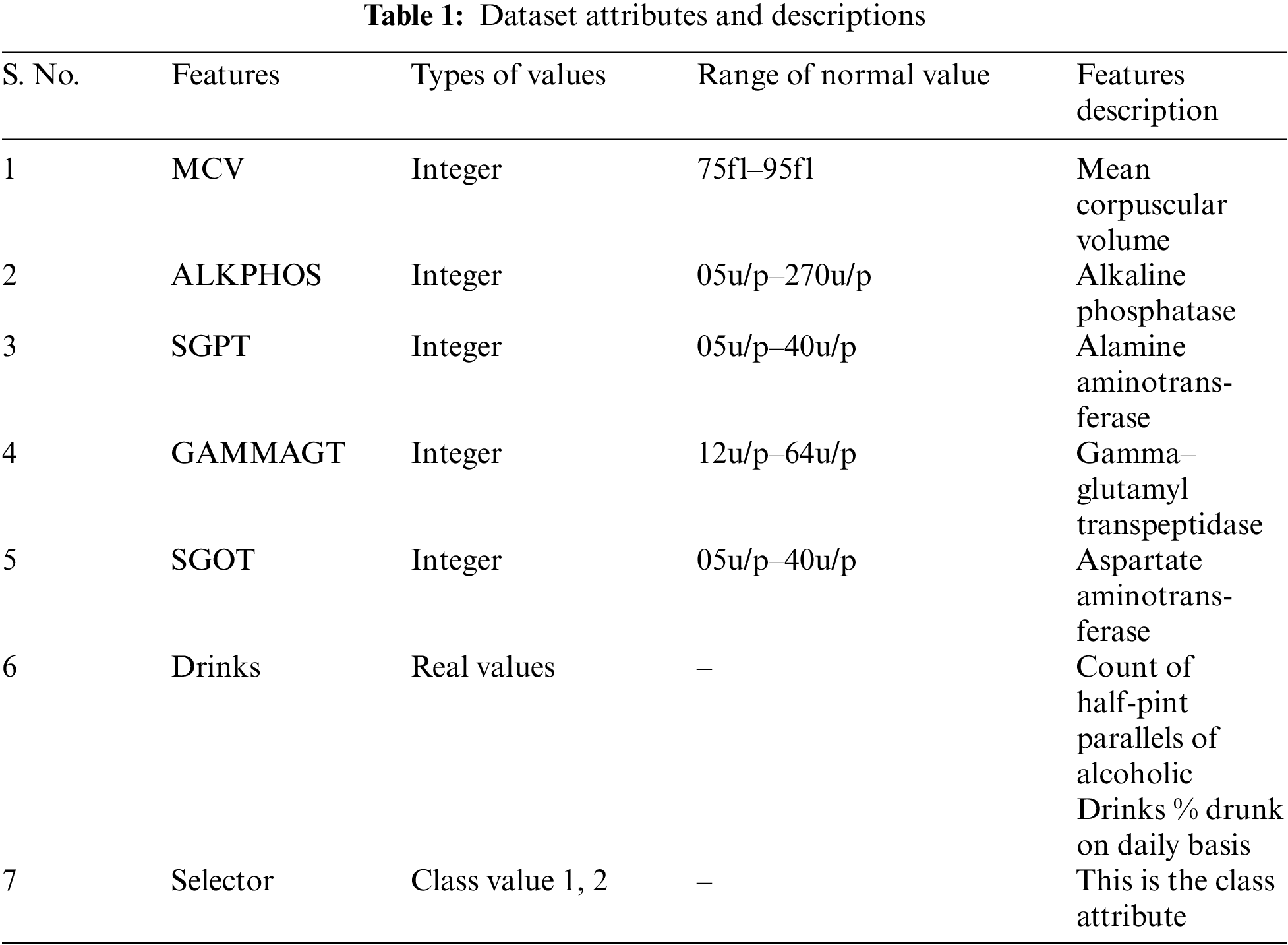
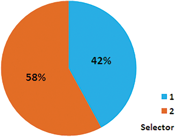
Figure 2: Percentage of selector 1 and 2

2.2 Performance Assessments Measures

In scientific studies, performance assessment is an important task to evaluate each utilized model. However, assessment measures used in this work, are binary classified, among these, first type are used for the assessment of error rate including RRSE [13] and RMSE [13,14], while other are used for the assessment of accuracy, e.g., accuracy [3], [15,16], MCC [17–19], recall [20,21], precision [22,23], specificity [5,24], F-measure [17,18], and G-measure [25,26]. Both accuracy measurement and error rate measurement are important factors in any model assessment for classification as well as in regression.

RMSE: It is the quadratic procuring decision that in addition registers the typical magnitude error,

RMSE=1n∑j=1n(yi−1)2(1)

RRSE: It is the square root of the relative squared error singular attenuation’s the error to similar scopes as the accountability being predicted,

RRSE=∑j=1n(Pij−Tj)2∑j=1n(Tj−T¯)2(2)

Specificity: It is calculated the number of concrete negatives that are correctly recognized,

Specificity=TNFP+TN(3)

Precision: It calculates the positive forecasts by the overall positive class value projected,

Precision=TPTP+FP(4)

Recall: It is the quotient of TP classes estimation to overall classes that are infected positive,

Recall=TPTP+FN(5)

MCC: It is a correlation coefficient that can be computed by all four values presented in the confusion matrix (CM),

MCC=(TN∗FN)−(FN∗FP)(FP+TP)(FN+TP)(TN+FP)(TN+FN)(6)

F-measure: It delivers the stability amongst precision and recall,

F−Measure=2∗Presision∗RecallPrecision+Recall(7)

G-measure: It is the permanency amide specificity and recall,

G−Measure=2∗Recall∗SpecificityRecall+Specificity(8)

Accuracy: It shows how much the prediction is accurate,

Accuracy=TP+TNTP+TN+FP+FN(9)

where, |yi − y| is the absolute error, the number of errors is represented by n, for record ji the objective value is Tj, Pij is the forecasted value by the precise sample I for j record, TP is the count of true-positive classification, the count of false-negative classification is presented by FN, count of true-negative classification is presented by TN, while the count of false-positive classifications is presented by FP.

2.3 Proposed Solution

The proposed model delivers better accuracy for liver disease prediction. The proposed model is depending on the implementation of the RF classifier to fulfill the contributions of this research. This work is done as mentioned in the following steps as well shown in the block diagram in Fig. 3:

1.    Elect a random sample from the particular dataset.

2.    Construct a decision tree for the individual model, and acquire forecasting results of the individual decision tree.

3.    Execute a majority voting mechanism for the individual forecasted outcome.

4.    Select the forecasted outcome with the high votes as the final forecast.

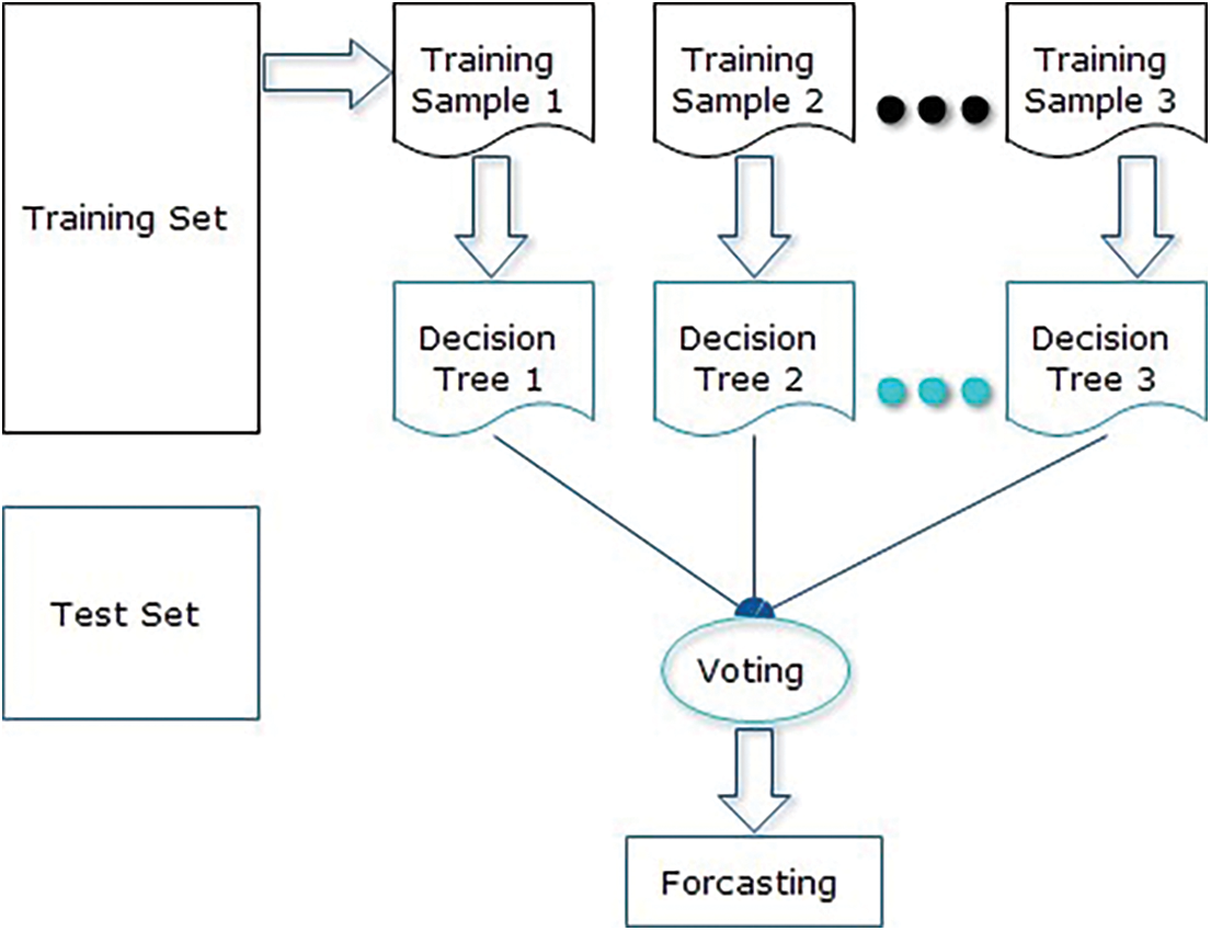
Figure 3: Proposed solution block diagram

The algorithm for the proposed solution in Fig. 3 is:

Let NTrees be the count of trees to build for an individual of NTrees iterations

1.    Elect a fresh bootstrap model from a training set.

2.    Develop an un-punned tree on this bootstrap.

3.    At every internal node, arbitrarily choose mtry predictor and decide the finest spilled utilizing only these predictions.

4.    Do not do cost complexity pruning. Save trees as is, together with those constructed thus far.

Here, split are selected according to a purity assessment criteria e.g., Gini index. NTrees means that create trees until the error no longer reduces, and for the selection of mtry try the recommendation defaults, half of them and twice them and pick the best.

The inclusive forecast is the majority vote (classification) from all independently trained trees. Fig. 4 shows the flow diagram of the projected algorithm.

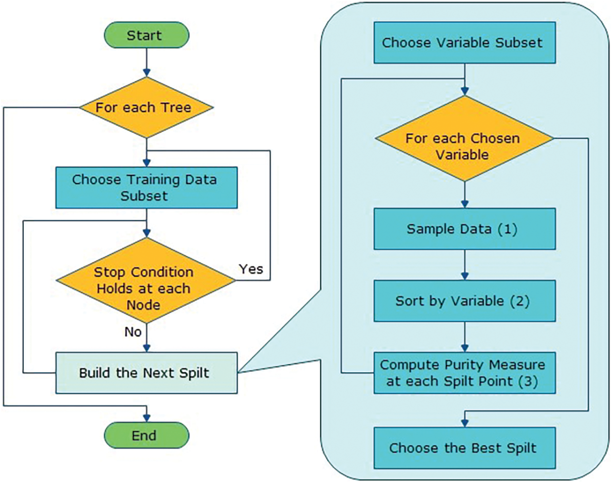
Figure 4: Flow diagram of the proposed solution

2.3.1 Random Forest (RF)

It is first projected by Tin Kam Ho of Bell Labs in 1995 [27], is an ensemble learning technique for regression and classification [28,29]. Leo Breiman and Adele Cutler [30] established RF, which is a supervised classification technique considered the utmost advanced ensemble learning technique accessible and is an extremely elastic classifier [3]. As the term proposes, this technique produces a forest with several trees [31,32]. In the forest, a large number of trees are the most dynamic, however, in the RF, the enormous number of trees in the timberland give better accuracy [7,20].

2.3.2 RF Pseudo Code

1)   Randomly choose, “k” features among total “m” features, where k ¡¡ m

2)   Amid the “k” features, find the node “d” by the best-fragmented fact.

3)   Divide the node into offspring nodes by the finest fragmented.

4)   Reprise 1 to 3 steps till “l” count of nodes has been grasped.

5)   Develop the forest by iterating steps 1 to 4 for “n” times to construct “n” number of trees.

The start of the RF technique surprises with arbitrarily selecting “k” features. These “k” features are selected among all “m” features. In the next phase, it uses the arbitrarily voted “k” types to discover the source node by employing the finest fragmented method. After that, it calculates the offspring nodes by the similar finest fragmented method. It will repeat the first 3 phases till it constructs the tree with a source node and takes the goal as the leaf node. As a final point, it will reprise 1 to 4 phases to produce “n” randomly generated trees. These arbitrarily generated trees from the RF.

2.3.3 RF Forecasting Pseudo Code

The following pseudo-code is used to achieve forecasting using a trained RF algorithm:

1)   Proceed with the test attributes and use the instructions of each arbitrarily produced decision tree to forecast the conclusion, and keeps the predicted conclusion.

2)   Compute the elects of individual forecasted objectives.

3)   Think through the successful voted forecasted target as the concluded forecasting from the RF.

The trained RF technique needs authorization to test features by the instructions of the arbitrary developed tree for prediction. Every RF will forecast different outcomes (results) for the same test feature.

At the same time given every forecasted target vote will be calculated. This can be assumed as:

Assuming a hundred arbitrary decision trees are estimated sure three novel targets, e.g., x, y, and z, at that point the votes of x is nothing yet out of 100 irregular decision trees, the number of trees gauge as x. Also, for the remainder of the two goals y and z, if x gets high votes. For instance, among hundred arbitrary decision trees, sixty trees are gauged as x, at that point, the last RF returns the x as the determined objective. This thought of the idea of voting is distinguished as majority voting.

2.4 Review of Other Employed Classifiers

This section contains a brief description of each utilized technique.

2.4.1 Multilayer Perceptron (MLPs)

MLPs are considered important classes of neural networks. MLP consists of three types of layers, e.g., input, hidden, and output layers [33,34]. A neural network works when information is available in the input layer. After that, the computation begins in a hidden layer by network neurons till output esteem is acquired at every one of the output neurons. An inception node is additionally included in the input layer which distinguishes the weight function [35].

2.4.2 Naïve Bayes (NB)

NB is a probabilistic algorithm that depends on Bayes theory with unbiasedness suppositions amid the forecasters [12,36]. NB model is fundamentally an exact easy to develop and apply to any dataset of huge data. The back likelihood, P(c—x) is taken from P(c), P(x), and P(x—c). The result of the estimation of a forecaster (x) on accepted class (c) is autonomous of the estimation of different forecasters.

2.4.3 Composite Hypercube on Iterated Random Projection (CHIRP)

CHIRP is a frequentative model consisting of three stages; covering, expecting, and discarding. It anticipated a reimbursement using the blight of algorithmic unpredictability, nonlinear recognizability, and dimensionality [37]. It is not the enhancement or adjustment of previous models, moreover, not cascading or hybridization of various techniques. CHIRP is depending on innovative packaging techniques. The accuracy of this model on usually employed neutral datasets beats the accuracy of competitors. The CHIRP employs the numeration compelling methods to treat with pull together 2D predictions, and chunks of quadrilateral spaces on those predictions that comprise the estimations from independent sets of information. CHIRP classifies these sets of forecasts and fragments them into an end gradient for adding new data points [38].

2.4.4 Average One Dependency Estimator (A1DE)

A1DE depends on probability and is mostly used for classification. It prospers incredibly exact classification by averaging complete slight space of various NB-like models, which have tinier individual assumptions than NB. The A1DE algorithm was fundamentally intended to address the property’s problems. It was proposed to discourse on the quality autonomy problem of the common NB classifier [39].

2.4.5 Support Vector Machine (SVM)

SVM is mostly used for pattern recognition, bio-photonics, and classification. It was designed for twofold classification, though; it can also be used for compound classifications [23,25]. For binary classification, the central fair of SVM is to depict a line among classes of data to abuse the distance of boundary line from data points insincere adjoining toward it. All things considered, if data is linearly indistinguishable, a mathematical function is used to change the data to a higher dimensional space to such an extent that it might get linear separable in the new space [40].

2.4.6 Decision Tree (J48)

J48 is utilized for classification and regression [15]. Also, conventionally used to shock the result of biasness as it is the deviation of Information Gain (IG). A property with the most prominent expansion distribution is appointed alive and well a tree as a breaking highlight. Gain Ratio (GR) based decision tree that beats IG-based outcome in terms of accuracy [4].

2.4.7 K-Nearest Neighbor (KNN)

KNN arranges the characteristics of attributes to gauge the grouping of test data, it groups the firsthand data from the new data to “k” nearest neighbor by negligible distance utilizing unmistakable distance functions, e.g., Minkowski Distance (MkD), Manhattan Distance (MD), and Euclidean Distance (ED) [9,41].

2.4.8 Forest by Penalizing Attributes (Forest-PA)

This algorithm works based on penalized attributes bootstrap tests, the persistence is to develop a collection of the most exact decision trees utilizing controlling the advantage of all non-class attributes introduced in the dataset, dissimilar to certain current methods that utilization a small chunk of the non-class attributes. At a near chance to help hearty variety, Forest-PA maintains hindrances to a particular characteristic that conveys the succeeding tree from the freshest tree. Forest-PA also improves the weight from ascribes that have not been attempted in the ensuing trees [42].

2.4.9 Credal Decision Tree (CDT)

This algorithm is a plan for classification dependent on in-accurate prospects and implausibility measures [43]. All through the developing technique of a CDT to avoid delivering an uncertain decision tree, another standard was introduced that is stopped due to the splitting of the decision tree once the absolute implausibility increases. The function used in the all-out faltered measurement can be transitively expressed [44,45].

3  Experimental Results

This Section contains the outcomes achieved for liver disease prescience using RF just as nine other ML classifiers. For testing and training, 10-FCV is utilized [23]. Experimental analyses show that, the error rates (accomplished through RMSE and RRSE) and accuracy (prevailing by methods for MCC, accuracy, recall, specificity, precision, F-measure, and G-measure).

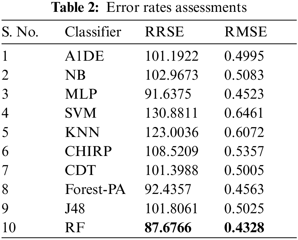
Here, right off the bat we examine the tests done to track down the least error rate evaluated by RRSE and RMSE accomplish, and discussed in Tab. 2, the detail utilized are listed in the second column, while the outcomes of RRSE and RMSE are individually presented in third and fourth columns respectively. It can be observed that RF outflanks the remaining classifiers regarding lessening error rates, outcomes are 0.4328 for RMSE and 87.6766 for RRSE. In the remainder of the classifiers, MLP creates better outcomes in decreasing both RMSE and RRSE, the separately results accomplished are 0.4532 and 91.6375.

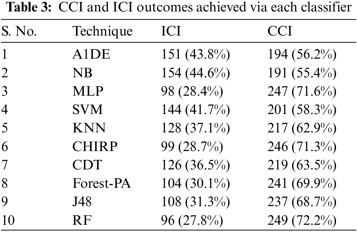
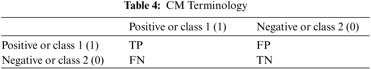
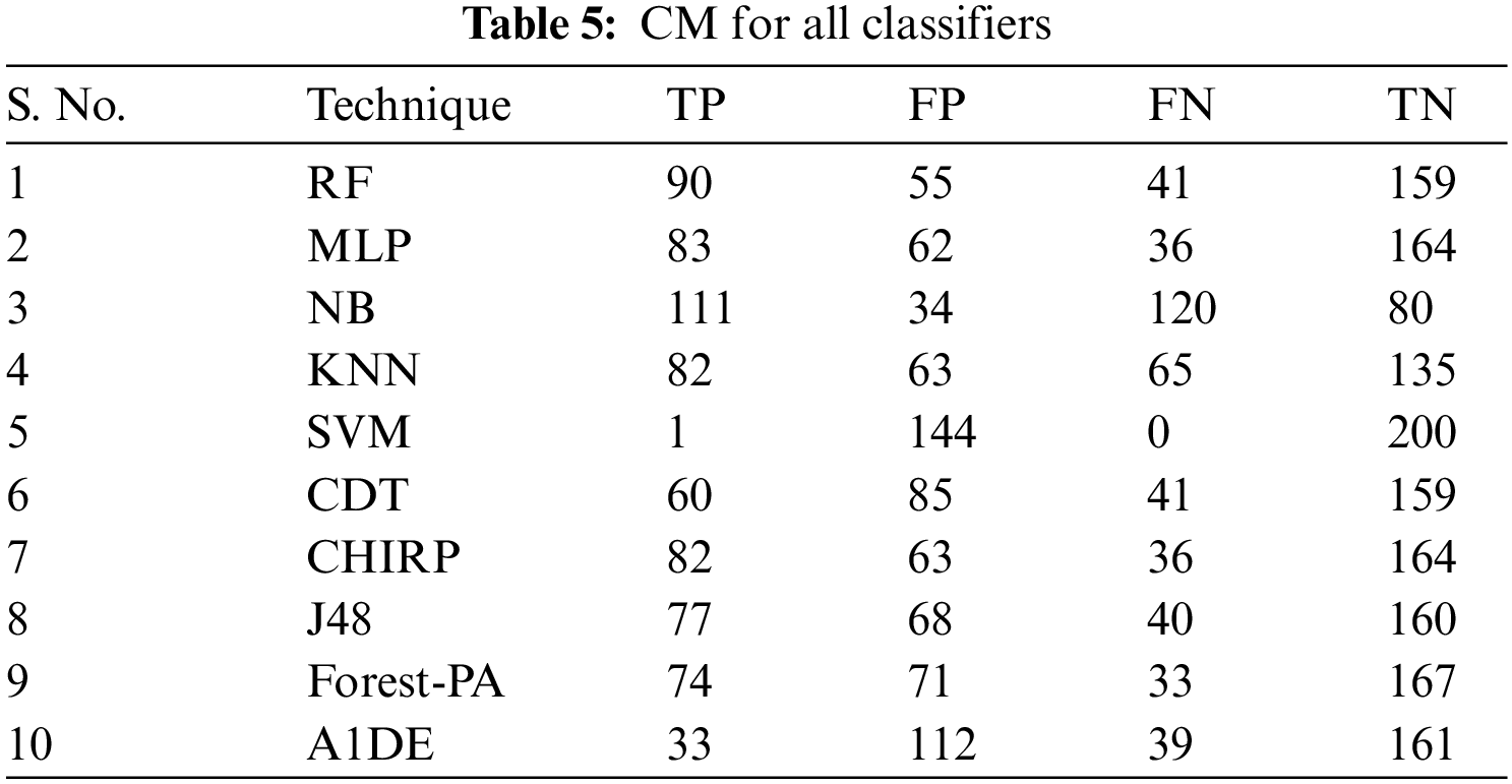
Tab. 3 presents the aspect of Incorrectly Classified Instances (ICI) Correctly Classified Instances (CCI) among a total of 345 instances. Better CCI shows the best performance of classifiers. Tab. 4 shows the terms used in the CM, while Tab. 5 shows the CM for every assessment evaluated during the experimentation. There is a binary classification for the prediction that is Positive (Class 1) and Negative (Class 2). Positive occurrence shows that the person is diseased while Negative is the representation of healthy prediction. In Tab. 4, TP shows the positive cases (the person is diseased), as well as FP also represents the positive cases. The positive cases predicted via RP are the persons who do not have any syndrome that is named a Type 1 error; therefore, this is named a Type 1 error. TN shows the negative cases (the person is not diseased) moreover, the FN also shows the negative cases, but the negative cases shown by FN are the persons who have the disease this is called a Type 2 error.

Tab. 6 shows the evaluated results of accuracy, recall, precision, specificity, F-measure, G-measure, and MCC relating to every individual classifier. The estimations of every measure are assessed using CM. The paramount exhibition of every classifier evaluated using each assessment metric is referenced in the bold text. This investigation shows that every classifier assesses through accuracy, MCC, specificity, F-measure, and RF outflanks different classifiers used in this work and accomplished better outcomes. The subtleties as indicated are introduced in Fig. 5, while Fig. 6 shows the accuracy subtleties. On assessing precision, the results of NB outperform the rest of the classifiers, while on G-measure and recall, SVM beats different classifiers utilized. The accuracy percentage difference (PD) of RF concerning other utilized classifiers is illustrated in Fig. 7, computed as:

PercentageDifference=(|V1−V2|(V1+V22))∗100.(10)

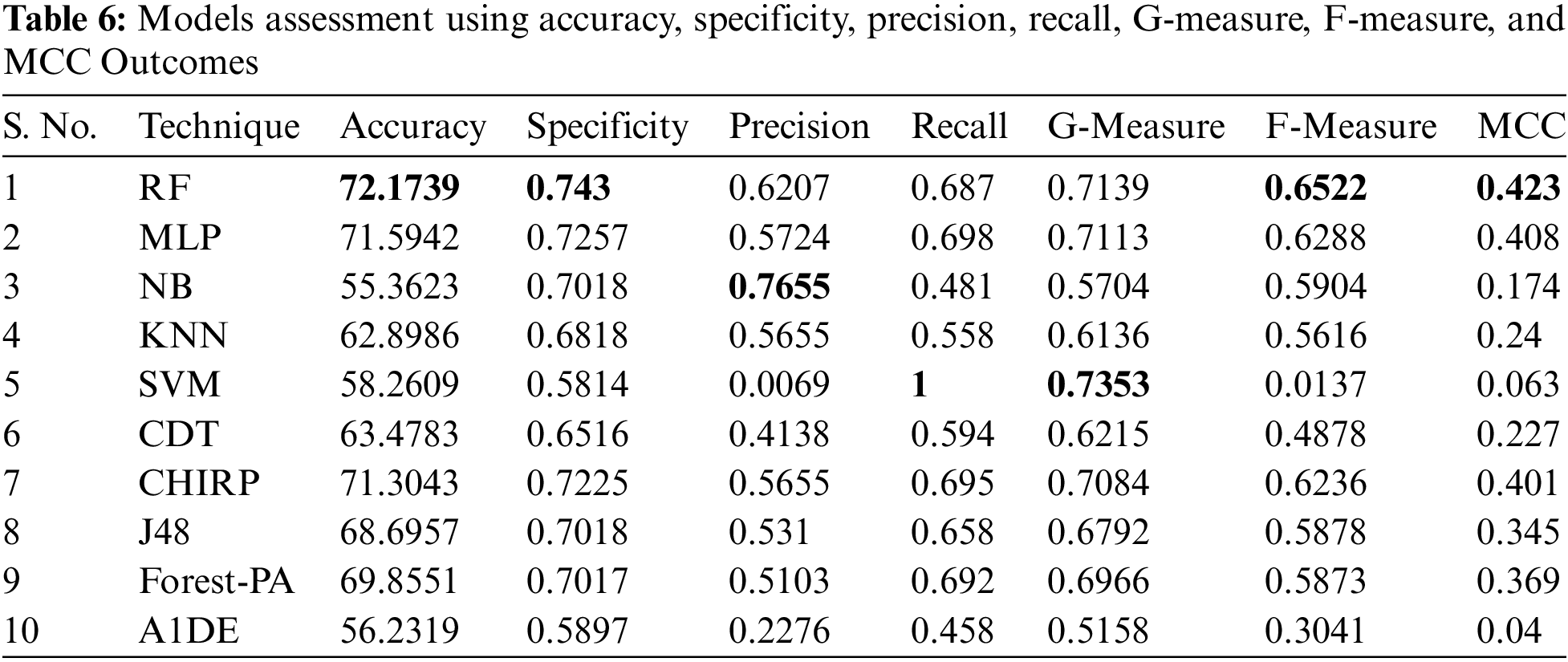
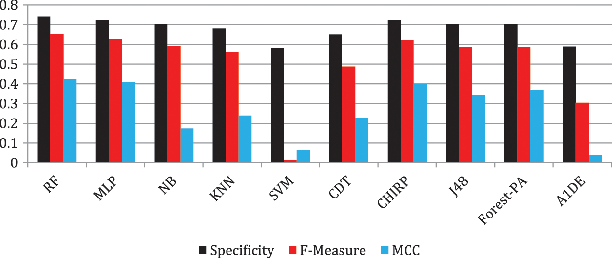
Figure 5: F-measure, specificity and MCC analysis representation

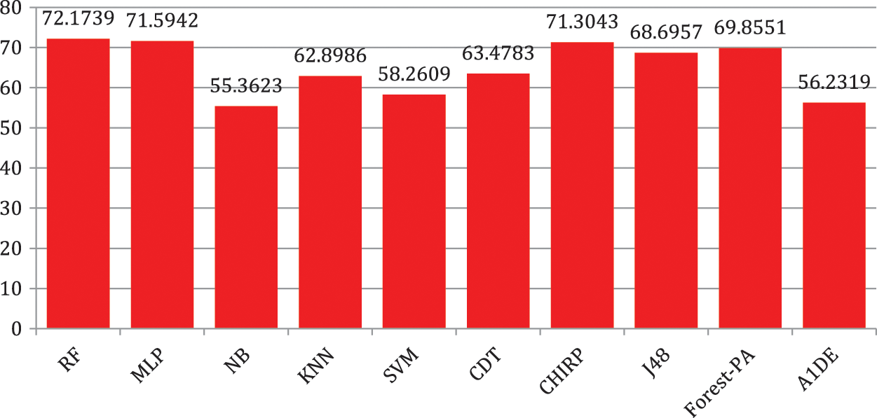
Figure 6: Accuracy representation

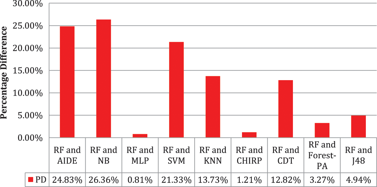
Figure 7: Percentage difference in accuracy of RF with other used classifiers

In Eq. (10), vi and vj are the values. Fig. 7 illustrates that there is limited variance between RF and CHIRP, and RF and MLP, which is 1.21 percent and 0.81 percent accordingly.

3.1 Discussion

As mentioned in the exploration RF leaves behind in contrast with other utilized techniques using reducing the error rate and increasing accuracy. Here, the question can arise that why RF beats other classifiers in both scenarios, e.g., reducing error rate and increasing accuracy. Just as there can be some features that may affect the validity of RF which are mentioned in the consequent section. Now the question may arise that why the performance of RF is better than other employed classifiers?

RF is a high dimensional classifier, to prevail in the assumption using the trained RF, needs to permit the test features by the information of individual self-assertively made trees [7,27]. RFs, anguish less overfitting to a particular dataset than basic trees. RFs built using blending the gauges of various trees, every one of which is prepared in partition, which gives significant inside assessments of solidarity, error, variable significance, and connection [17,46]. Accuracy and variable importance are generated automatically [47]. Unlike other models, e.g., Boosting, where the main models are trained and collective by a refined weighting structure, normally the trees are trained autonomously and the forecasts of the trees are joint through averaging [27,30].

3.1.1 Model Preparation

In this work, a model for liver disease prediction is recommended, assessed, and indorsed to test and compare the achievements of RF with NB, A1DE, SVM, MLP, KNN, CDT, J48, Forest-PA, and CHIRP classifiers, the overall outcomes exposed that RF is a prominent classifier among other utilized classifiers, for the early prediction of liver disease.

3.1.2 Model Evaluation

We compare RF with NB, A1DE, SVM, MLP, KNN, CDT, J48, Forest-PA, and CHIRP classifiers, and found that the RF classifier is the most optimal for the prediction of liver syndromes.

3.1.3 Objectives Accomplished

•   To explore RF for liver disease prediction, which will increase the accuracy and lessen the error rate in timely forecasting.

•   To compare the results of RF with nine other well-known classifiers to test that the proposed classifier is the most optimum result for timely and accurate prediction of liver diseases.

3.2 Threats to Validity

This Section comprises the impacts that may agony the influence of this work.

3.2.1 Internal Validity

The investigation of this work is based on continuing assorted and exceptionally familiar assessments that are utilized in the past in different research work. Amid these norms, a few are utilized to evaluate the accuracy, whereas, some are used to evaluate the error rate. In this way, the threat can be that the restoration of new assessment criteria as a trade for used criteria can diminish the accuracy. Besides, the classifiers used in this work can be replaced using a few freshest methods or can be merged that can collect improved results when contrasted with the utilized methods.

3.2.2 External Validity

This work directed analysis of the dataset taken from UCI. The threat may be due to the state of involving the extended classifiers in other existent data formed from the different clinical associations may trouble the results while increasing the error rates. Moreover, the utilized method potentially will not be fit for collecting improved figures in results through certain extra datasets. Consequently, this work focused on datasets accessible at UCI to evaluate the prominence of the used methods.

3.2.3 Construct Validity

A comparison of various ML methods with each other is done in this work on the dataset taken from the UCI repository on different assessment measures. The selection of techniques used in this work is based on the progressive characteristics of the other techniques used in the last decades. However, it tends to be a threat on the off chance that we put on some other new methods the results can be improved presumably than they utilize methods. Moreover, on the off chance that we utilize the training and testing models or we reduce or increment the count of FCV for the experimentation can likewise be the reason to diminish the error rate. The freshest assessment criteria can likewise create improved results that can beat current achieved results.

4  Conclusion

Liver syndromes are expanding on a routine, and it is difficult to predict these infirmities in the early stages. Analysts have used an enormous number of ML methods to predict such illnesses at the underlying stage, yet, there is a need to improve accuracy to decrease error rates in the proposed methods. However, in this work, the RF classifier is explored for the early prediction of liver disease. This classifier is benchmarked with nine other well-known classifiers including MLP, NB, A1DE, SVM, CDT, KNN, J48, Forest-PA, and CHIRP using standard assessment measures that comprise RRSE, RMSE, recall, accuracy, precision, MCC, specificity, G-measure, and F-measure. The concluded analysis describes that RF outperforms other classifiers in terms of increasing accuracy and reducing the error rate. RRSE and RMSE results of RF are 87.6766 and 0.4328 similarly, while the percentage accuracy is 72.1739. This study suggests RF for the early and optimal prophecy of liver syndromes. In the future, we can ensemble RF with some other advanced models that can help to improve the accuracy and reduce the error rate. Furthermore, the outcomes of this study can be the benchmark for other researchers working in the same area.

5  Significance of the Study

In this research, we explore an RF classifier for the early forecasting of liver disease. The outcomes of RF are compared with nine other ML classifiers on the liver dataset taken from the UCI repository. The dataset contains 345 instances of affected and non-affected persons. The recommendation of this work presents that RF is the better classifier among other used classifiers that can be used by specialists to eliminate treatment and investigative errors.

Acknowledgement: Authors would like to acknowledge the support of the Deputy for Research and Innovation-Ministry of Education, Kingdom of Saudi Arabia for this research through a grant (NU/IFC/ENT/01/014) under the institutional Funding Committee at Najran University, Kingdom of Saudi Arabia.

Funding Statement: Authors would like to acknowledge the support of the Deputy for Research and Innovation-Ministry of Education, Kingdom of Saudi Arabia for this research at Najran University, Kingdom of Saudi Arabia.

Conflicts of Interest: The authors declare that they have no conflicts of interest to report regarding the present study.

1https://archive.ics.uci.edu/ml/datasets/liver+disorders

References

1. A. N. Arbain and B. Y. P. Balakrishnan, “A comparison of data mining algorithms for liver disease prediction on imbalanced data,” International Journal of Data Science and Advanced Analytics, vol. 1, no. 1, pp. 1–11, 2019. [Google Scholar]
2. G. Shiha, M. Korenjak, W. Eskridge, T. Casanovas, P. Velez-Moller et al., “Redefining fatty liver disease: An international patient perspective,” The Lancet Gastroenterology and Hepatology, vol. 6, no. 1, pp. 73–79, 2021. [Google Scholar]
3. N. Nahar and F. Ara, “Liver disease prediction by using different decision tree techniques,” International Journal of Data Mining and Knowledge Management Process, vol. 8, no. 2, pp. 01–09, 2018. [Google Scholar]
4. T. Marjot, G. J. Webb, A. S. Barritt, A. M. Moon, Z. Stamataki et al., “COVID-19 and liver disease: Mechanistic and clinical perspectives,” Nature Reviews Gastroenterology and Hepatology, vol. 18, no. 5, pp. 348–364, 2021. [Google Scholar]
5. M. Abdar, N. Y. Yen and J. C. S. Hung, “Improving the diagnosis of liver disease using multilayer perceptron neural network and boosted decision trees,” Journal of Medical and Biological Engineering, vol. 38, no. 6, pp. 953–965, 2018. [Google Scholar]
6. M. Abdar, M. Zomorodi-Moghadam, R. Das and I. H. Ting, “Performance analysis of classification algorithms on early detection of liver disease,” Expert Systems with Applications, vol. 67, no. 1, pp. 239–251, 2017. [Google Scholar]
7. L. Lau, Y. Kankanige, B. Rubinstein, R. Jones, C. Christophi et al., “Machine-learning algorithms predict graft failure after liver transplantation,” Transplantation, vol. 101, no. 4, pp. e125–e132, 2017. [Google Scholar]
8. B. Khan, R. Naseem, M. Ali, M. Arshad and N. Jan, “Machine learning approaches for liver disease diagnosing,” International Journal of Data Science and Advanced Analytics, vol. 1, no. 1, pp. 27–31, 2019. [Google Scholar]
9. U. R. Acharya, H. Fujita, S. Bhat, U. Raghavendra, A. Gudigar et al., “Decision support system for fatty liver disease using GIST descriptors extracted from ultrasound images,” Information Fusion, vol. 29, no. 1, pp. 32–39, 2016. [Google Scholar]
10. U. R. Acharya, H. Fujita, V. K. Sudarshan, M. R. K. Mookiah, J. EW Koh et al., “An integrated index for identification of fatty liver disease using radon transform and discrete cosine transform features in ultrasound images,” Information Fusion, vol. 31, no. 1, pp. 43–53, 2016. [Google Scholar]
11. H. Sun and R. Grishman, “Lexicalized dependency paths based supervised learning for relation extraction,” Computer Systems Science and Engineering, vol. 43, no. 3, pp. 861–870, 2022. [Google Scholar]
12. T. R. Baitharu and S. K. Pani, “Analysis of data mining techniques for healthcare decision support system using liver disorder dataset,” Procedia Computer Science, vol. 85, pp. 862–870, 2016. [Google Scholar]
13. B. Khan, R. Naseem, F. Muhammad, G. Abbas and S. Kim, “An empirical evaluation of machine learning techniques for chronic kidney disease prophecy,” IEEE Access, vol. 8, pp. 55012–55022, 2020. [Google Scholar]
14. P. Guo, T. Liu, Q. Zhang, L. Wang, J. Xiao et al., “Developing a dengue forecast model using machine learning: A case study in China,” PLoS Neglected Tropical Diseases, vol. 11, no. 10, pp. 1–22, 2017. [Google Scholar]
15. T. F. Yip, A. J. Ma, V. S. Wong, Y. K. Tse, H. Y. Chan et al., “Laboratory parameter-based machine learning model for excluding non-alcoholic fatty liver disease (NAFLD) in the general population,” Alimentary Pharmacology and Therapeutics, vol. 46, no. 4, pp. 447–456, 2017. [Google Scholar]
16. T. Menzies, A. Dekhtyar, J. Distefano and J. Greenwald, “Problems with precision: A response to Comments on “data mining static code attributes to learn defect predictors”,” IEEE Transactions on Software Engineering, vol. 33, no. 9, pp. 637–640, 2007. [Google Scholar]
17. S. Khan, R. Ullah, A. Khan, N. Wahab, M. Bilal et al., “Analysis of dengue infection based on Raman spectroscopy and support vector machine (SVM),” Biomedical Optics Express, vol. 7, no. 6, pp. 2249, 2016. [Google Scholar]
18. H. Jin, S. Kim and J. Kim, “Decision factors on effective liver patient data prediction,” Biomedical Optics Express, vol. 6, no. 4, pp. 167–178, 2014. [Google Scholar]
19. D. A. E. H. Omran, A. B. H. Awad, M. A. E. R. Mabrouk, A. F. Soliman and A. O. A. Aziz, “Application of data mining techniques to explore predictors of HCC in Egyptian patients with HCV-related chronic liver disease,” Asian Pacific Journal of Cancer Prevention, vol. 16, no. 1, pp. 381–385, 2015. [Google Scholar]
20. A. Iqbal, S. Aftab, U. Ali, Z. Nawaz, L. Sana et al., “Performance analysis of machine learning techniques on software defect prediction using NASA datasets,” International Journal of Advanced Computer Science and Applications, vol. 10, no. 5, pp. 300–308, 2019. [Google Scholar]
21. H. Tong, B. Liu and S. Wang, “Software defect prediction using stacked denoising autoencoders and two-stage ensemble learning,” Information and Software Technology, vol. 96, no. 1, pp. 94–111, 2018. [Google Scholar]
22. A. Alsaeedi and M. Z. Khan, “Software defect prediction using supervised machine learning and ensemble techniques: A comparative study,” Journal of Software Engineering and Applications, vol. 12, no. 8, pp. 85–100, 2019. [Google Scholar]
23. J. Chen, Y. Yang, K. Hu, Q. Xuan, Y. Liu et al., “Multiview transfer learning for software defect prediction,” IEEE Access, vol. 7, no. 1, pp. 8901–8916, 2019. [Google Scholar]
24. Q. Song, Y. Guo and M. Shepperd, “A comprehensive investigation of the role of imbalanced learning for software defect prediction,” IEEE Transactions on Software Engineering, vol. 45, no. 12, pp. 1253–1269, 2019. [Google Scholar]
25. M. M. Saritas, “Performance analysis of ann and naive Bayes classification algorithm for data classification,” International Journal of Intelligent Systems and Applications in Engineering, vol. 7, no. 2, pp. 88–91, 2019. [Google Scholar]
26. C. H. Wu, S. C. Kao, C. H. Shih and M. H. Kan, “Open data mining for Taiwan’s dengue epidemic,” Acta Tropica, vol. 183, no. 1, pp. 1–7, 2018. [Google Scholar]
27. T. K. Ho, “Random decision forests,” in Proc. of 3rd Int. Conf. on Document Analysis and Recognition, Montreal, Canada, vol. 1, no. 1, pp. 278–282, 1995. [Google Scholar]
28. D. Bowes, T. Hall and J. Petrić, “Software defect prediction: Do different classifiers find the same defects?,” Software Quality Journal, vol. 26, no. 2, pp. 525–552, 2018. [Google Scholar]
29. A. Gupte, S. Joshi, P. Gadgul and A. Kadam, “Comparative study of classification algorithms used in sentiment analysis,” International Journal of Computer Science and Information Technologies, vol. 5, no. 5, pp. 6261–6264, 2014. [Google Scholar]
30. T. M. Carvajal, K. M. Viacrusis, L. F. T. Hernandez, H. T. Ho, D. M. Amalin et al., “Machine learning methods reveal the temporal pattern of dengue incidence using meteorological factors in metropolitan Manila, Philippines,” BMC Infectious Diseases, vol. 18, no. 1, pp. 1–15, 2018. [Google Scholar]
31. A. Gulia, R. Vohra and P. Rani, “Liver patient classification using intelligent techniques,” International Journal of Computer Science and Information Technologies, vol. 5, no. 4, pp. 5110–5115, 2014. [Google Scholar]
32. S. Picek, A. Heuser and S. Guilley, “Template attack versus Bayes classifier,” Journal of Cryptographic Engineering, vol. 7, no. 4, pp. 343–351, 2017. [Google Scholar]
33. A. Naik and L. Samant, “Correlation review of classification algorithm using data mining tool: Weka, rapidminer, tanagra, orange and knime,” Procedia Computer Science, vol. 85, pp. 662–668, 2016. [Google Scholar]
34. K. A. Otunaiya and G. Muhammad, “Performance of datamining techniques in the prediction of chronic kidney disease,” Procedia Computer Science, vol. 7, no. 2, pp. 48–53, 2019. [Google Scholar]
35. B. Khan, R. Naseem, M. A. Shah, K. Wakil, A. Khan et al., “Software defect prediction for healthcare big data: An empirical evaluation of machine learning techniques,” Journal of Healthcare Engineering, vol. 2021, no. 1, pp. 1–16, 2021. [Google Scholar]
36. A. B. Nassif, D. Ho and L. F. Capretz, “Towards an early software estimation using log-linear regression and a multilayer perceptron model,” Journal of Systems and Software, vol. 86, no. 1, pp. 144–160, 2013. [Google Scholar]
37. C. Davi, A. Pastor, T. Oliveira, F. B. de Lima Neto, U. Braga-Neto et al., “Severe dengue prognosis using human genome data and machine learning,” IEEE Transactions on Biomedical Engineering, vol. 66, no. 10, pp. 2861–2868, 2019. [Google Scholar]
38. E. K. Hashi, M. S. Uz Zaman and M. R. Hasan, “An expert clinical decision support system to predict disease using classification techniques,” in Int. Conf. on Electrical, Computer and Communication Engineering, Cox’s Bazar, Bangladesh, pp. 396–400, 2017. [Google Scholar]
39. L. Wilkinson, A. Anand and D. N. Tuan, “CHIRP: A new classifier based on composite hypercubes on iterated random projections,” in Proc. of the 17th ACM SIGKDD Int. Conf. on Knowledge Discovery and Data Mining, New York, United State, pp. 6–14, 2011. [Google Scholar]
40. E. Byvatov and G. Schneider, “Support vector machine applications in bioinformatics,” Applied Bioinformatics, vol. 2, no. 2, pp. 67–77, 2003. [Google Scholar]
41. H. Arslan and H. Arslan, “A new covid-19 detection method from human genome sequences using cpg island features and knn classifier,” Engineering Science and Technology, an International Journal, vol. 24, no. 4, pp. 839–847, 2021. [Google Scholar]
42. Q. He, Z. Xu, S. Li, R. Li, S. Zhang et al., “Novel entropy and rotation forest-based credal decision tree classifier for landslide susceptibility modeling,” Entropy, vol. 21, no. 2, pp. 1–24, 2019. [Google Scholar]
43. J. A. Dhanraj, B. Lingampalli, M. Prabhakar, A. Sivakumar, B. Krishnamurthy et al., “A credal decision tree classifier approach for surface condition monitoring of friction stir weldment through vibration patterns,” Materials Today: Proceedings, vol. 46, pp. 1127–1133, 2021. [Google Scholar]
44. A. Arabameri, N. Sadhasivam, H. Turabieh, M. Mafarja, F. Rezaie et al., “Credal decision tree based novel ensemble models for spatial assessment of gully erosion and sustainable management,” Scientific Reports, vol. 11, no. 1, pp. 1–18, 2021. [Google Scholar]
45. C. J. Mantas and J. Abellán, “Analysis and extension of decision trees based on imprecise probabilities: Application on noisy data,” Expert Systems with Applications, vol. 41, no. 5, pp. 2514–2525, 2014. [Google Scholar]
46. M. Denil, D. Matheson and N. De Freitas, “Narrowing the gap: Random forests in theory and in practice,” in Proc. of the 31st Int. Conf. on Machine Learning, Beijing, China, pp. 665–673, 2014. [Google Scholar]
47. M. Hosseinpour-Zarnaq, M. Omid and E. Biabani-Aghdam, “Fault diagnosis of tractor auxiliary gearbox using vibration analysis and random forest classifier,” Information Processing in Agriculture, vol. 9, no. 1, pp. 60–67, 2022. [Google Scholar]
Cite This Article
Copyright © 2023 The Author(s). Published by Tech Science Press.
This work is licensed under a Creative Commons Attribution 4.0 International License , which permits unrestricted use, distribution, and reproduction in any medium, provided the original work is properly cited.
Downloads
Citation Tools