Time Series Forecasting Fusion Network Model Based on Prophet and Improved LSTM

1  Introduction

Univariate and multivariate time series data forecasting (TSF) and analysis are widely available in various fields of production and life, such as energy [1,2], environment [3], atmosphere [4], stock-stock index finance [5], geographical and Physical Sciences [6], public health [7], Urban Power and Transportation Field [8], Industrial Manufacturing and Production Field [9], Network, Cloud and Internet of Things [10]. In recent years, atmospheric and environmental issues have become increasingly severe, and relevant policies and measures have been introduced one after another. Environmental protection departments and related companies have gradually shifted their perspectives to effective supervision and data mining and predictive analysis of the atmosphere, environment and energy. Therefore, time series prediction models and algorithms that can adapt to higher dimensional data sets in this field and can guarantee relatively high accuracy are the current focus of exploration and research in this field, as well as the research focus of this article.

The traditional time series forecasting method fits the historical time trend curve by establishing an appropriate mathematical model, and predicts the trend curve of the future time series according to the built model. Common models include Auto-Regression Moving Average (ARMA), Vector Auto-Regression (VAR), prophet, etc. [11]. Traditional time series methods rely on relatively simple data, and only need historical time series trend curves to build a model, so it can be applied to a variety of scenarios, and the model is more general. However, traditional time series forecasting methods often only accept univariate [12], or often face the problem of lag, that is, the predicted value is several time units later than the true value [13].

In order to improve the accuracy of prediction, machine learning algorithms and deep learning are introduced into time series prediction. These methods select features that may affect the predicted value according to specific application scenarios, introduce these features into the model, and apply machine learning classification or regression models to perform forecast [14,15]. In order to extract features, machine learning and deep learning methods require multiple dimensions of data. The prediction accuracy is higher and the established model is more complex, but the model is often not general enough. It is necessary to re-extract features and build models for different application scenarios. In reality forecasting, machine learning and deep learning methods are often combined with traditional time series forecasting methods, such as Liang et al. [16] combined with Prophet and support vector regression (SVR) models to predict seasonal manufacturing time series demand. The hybrid Prophet-SVR method is a fitting of machine learning and traditional methods. This method can not only customize the influence of holidays and seasons, but also consider prediction residuals to improve prediction accuracy. At the same time, deep learning methods and machine learning methods can also be integrated and improved, such as Ma et al. [9,17] combining LSTM networks and support vector machines (SVM) to perform power system data jumper faults forecast, focus on using the LSTM network to obtain the time characteristics of multi-source data, and the performance in the extraction of long-term time series features. In summary, see Tab. 1 for the classification of time series data prediction methods.

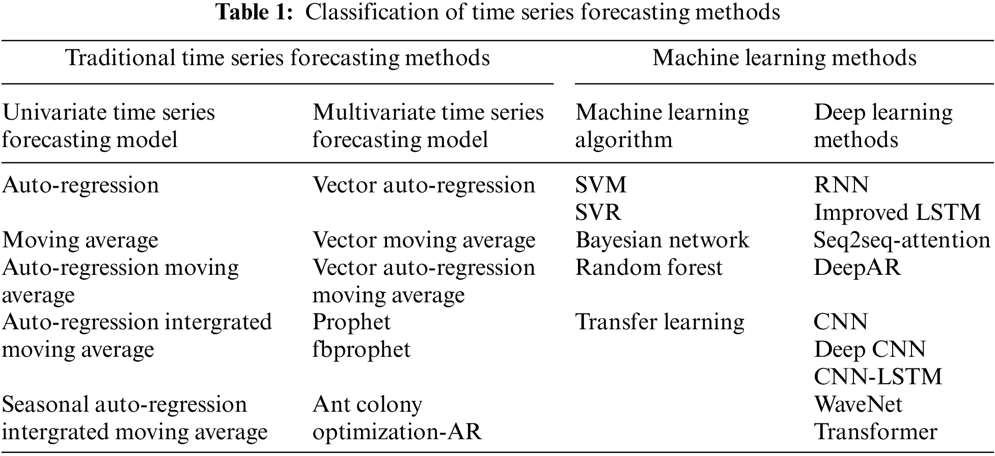
In the traditional multivariate time series forecasting model, the prophet algorithm can not only deal with the case of some outliers in the time series, but also the case of some missing values [18], and it can also predict the future trend of the time series almost automatically [19]. For machine learning models, the application of the model needs to find specific methods for specific problems [12], such as temperature prediction, whether the data has an obvious seasonal trend, whether there is a gradual upward trend, etc. If the model can be constructed directly from the observed features, the final prediction effect may be better than the complex sequence learning model. Among deep learning methods, convolutional neural network models (CNN) can be applied to time series forecasting, and at the same time, there are many types of CNN network models that can be used for each specific type of time series forecasting problem. However, such methods often show problems such as not supporting sequence input, large memory requirements, and omission of causal features of time series data [17]. Both LSTM and transformer are universal time series forecasting models. Although transformer is more widely used in the field of natural language processing (NLP), it can still be used for time series forecasting, but different time series data have their own characteristics, such as financial time series. The inherent laws of data and meteorological time series data are different, and a general sequence learning model may not be able to obtain satisfactory results, especially when there is not enough training data [20]. When the amount of data is not large, combining feature engineering and applying ensemble learning or transfer learning methods to obtain prediction results is better than directly applying models such as LSTM [21]. When the amount of data is slightly larger, we should consider using a priori using knowledge to modify the architecture of deep learning models such as LSTM and Transformer can also obtain better prediction results [22].

As a variant of recurrent neural network (RNN), LSTM has better iterative and deep structure, and adopts a special gated structure to overcome the shortcomings of RNN. With the improvement of hardware performance and computing power, LSTM and its variants excel in time series forecasting. Therefore, this paper proposes a deep learning framework for multivariate time series prediction that combines Prophet and improved LSTM units, named P-gLSTNet. Expect this model to outperform traditional or general models like LSTM, ARIMA, and Prophet.

2  Methods and Materials

2.1 Prophet Model

Prophet is a model for time series characteristics and change laws that was open sourced by Facebook in 2017 [16]. It is a data prediction tool based on Python and R languages. The two most critical points in the application of Prophet are the complexity of data and the evaluation of prediction results. The advantage of this model is that Prophet can fit seasonality by modifying seasonal parameters, and fit trend information by modify trend parameters, fit holiday information by specify holidays, etc. The essence of the model is an auto-additive regression cyclic structure model composed of four components, as shown in Fig. 1 below. Different trends of the time series are fitted with different parts, and the whole time series model is formed after superposition. The curve fitting is optimized based on L-BGFS to obtain the maximum a posteriori-estimate of each parameter.

Figure 1: Schematic diagram of the prophet model structure

From previous experimental research, the Prophet algorithm is based on the fitting of decomposed time series (that is, traditional methods) and machine learning methods. The time tasks used for prediction often have the following characteristics: reflecting in certain data samples of relatively stable frequency with a relatively fixed frequency in the time period; reflecting the stable and repeating general seasonal changes or other changes; reflecting the unknown and irregular mutation of holidays; reflecting the rational existence of missing data and data Abnormal; reflecting a situation that exhibits a reasonable change in trend; reflecting a trend that exhibits a linear or non-linear growth curve, or may reach a natural limit or saturation. Based on the above characteristics, the model focuses on two key points to make up for the limitations, missing values and flexibility of traditional time series models in the data processing process. Its core is to analyze various time series data characteristics such as periodicity, trend, holiday effect, seasonality and so on. The satisfaction of the trend term is achieved by linear piecewise fitting, and mutation points can be added manually or automatically selected by an algorithm; the satisfaction of the periodic term can be achieved by using Fourier series to establish a periodic model, its basic form is expressed as (1):

y(t)=g(t)+s(t)+h(t)+ϵt(1)

Among them, g(t) is a trend function, which is used to analyze aperiodic changes in time series; s(t) represents periodic changes, such as a year or a week; h(t) represents the impact of accidental factors at special time nodes, ε is a random fluctuation, which represents the error effect that the model does not consider.

(1)   Trend term: Trend growth in the Prophet model is similar to racial growth. Facebook employs a modified logistic growth model, where the saturation value changes dynamically over time, and the growth rate also changes with the relevant factors, its basic form is expressed as (2):

g(t)=C(t)1+exp⁡(−(k+a(t)Tδ)⋅(t−(m+a(t)Tγ)))(2)

(2)   Periodic term: The Prophet model constructs a periodic model by introducing Fourier series, and its basic form is expressed as (3):

s(t)=∑n=1N(ancos(2πntP)+bnsin(2πntP))(3)

where P is the period length of the time series, N represents the number of periods, and an, bn are the parameters to be estimated.

Compared with other time series models, the main advantage of the Prophet model is that it can flexibly adjust the periodic trend to meet the assumption of trend items in the experimental process; it can accommodate the diversity of data forms, and accommodate irregular intervals and missing values; it can be fitted quickly; it can have good modifiability, allowing analysts to improve its internal parameters.

Taking a common time series scenario as an example, black represents the original time series discrete points, the dark blue line represents the value obtained by fitting the time series, and the light blue line represents a confidence interval of the time series. This is the so-called reasonable upper and lower bounds. What prophet does is:

(1)   Step1: Enter the timestamp and corresponding value of a known time series;

(2)   Step2: Enter the length of the time series to be predicted;

(3)   Step3: Output future time series trends.

(4)   Step4: The output result can provide necessary statistical indicators, including fitting curve, upper bound and lower bound. It is also possible to increase seasonal processing. As shown in Fig. 2 below, the right side is the fitting curve for adding seasonal addition and multiplication processing.

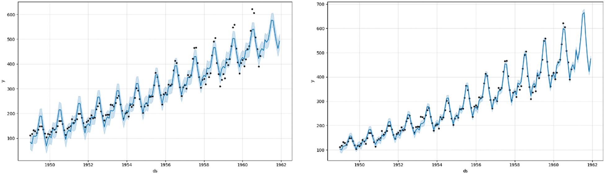
Figure 2: Examples of time series forecasting algorithms based on prophet

2.2 Long and Short-term Memory (LSTM) Model

Compared with RNN, LSTM can solve the problem of gradient disappearance and gradient explosion, but it is still not a more ideal unit structure [23]. Gate recurrent unit (GRU) merged the forget gate and the input gate into one “update gate”. At the same time, the unit state and hidden state were merged, and some other changes were made. The resulting model is simpler than the standard LSTM model and has been widely used. Using the improved ideas of GRU, comparing and optimizing the prediction models and methods of multivariate time series data, the neural network with improved LSTM unit is selected to build the prediction model. First of all, in the traditional LSTM cell, the input gate, forget gate and output gate all add the unit state information at the previous moment, so that the unit state information is fully utilized in the “gate”, and the input ratio is obtained according to the forgetting ratio [24].

Figs. 3 and 4 show the structure of the LSTM unit and the LSTM chain before and after the improvement. Where Xt is the input value, ht is the output value, tanh and σ (Sigmod) are the activation functions, and × and + represent the forget gate, input gate and output gate in the unit structure. Design a more efficient long and short-term memory neural network unit by improving the correlation function and the state of the “gate”, thereby optimizing the logic architecture of the LSTM layer of the neural network.

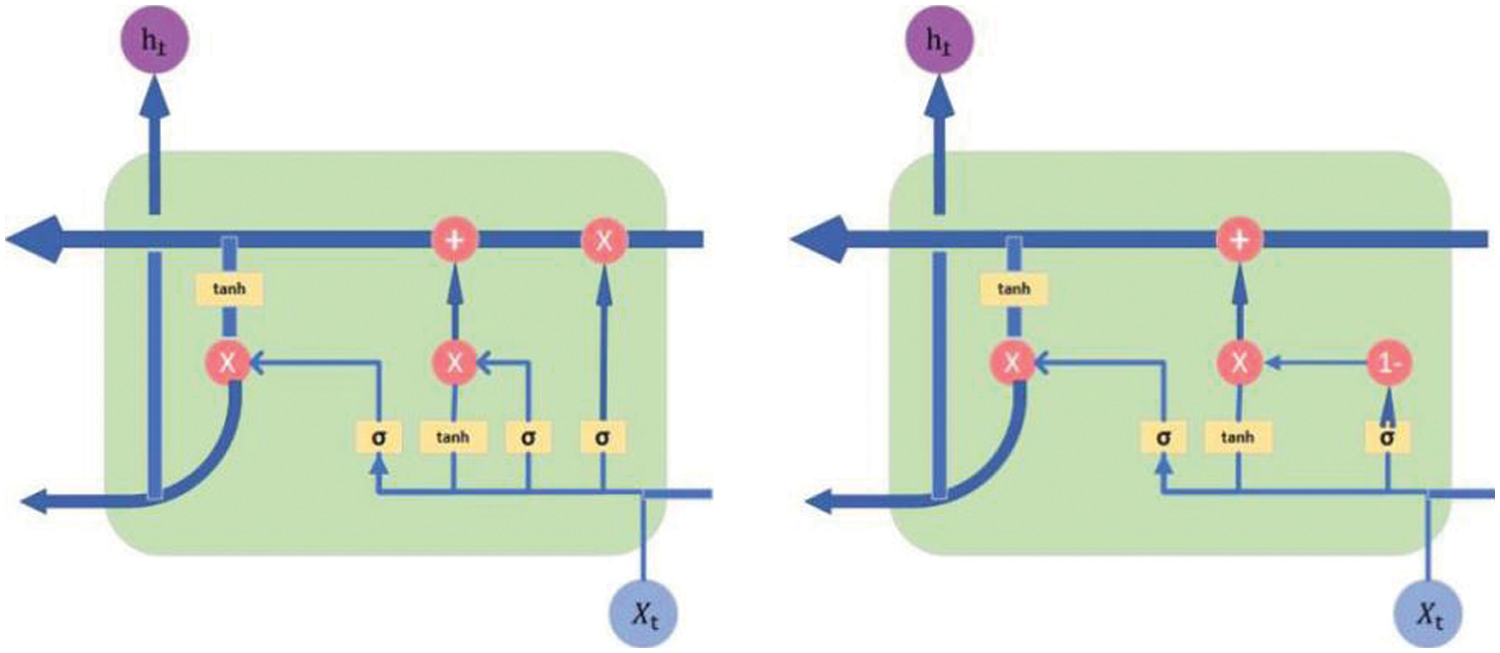
Figure 3: Improved LSTM unit structure diagram (The picture on the left is before improvement, and the picture on the right is after improvement)

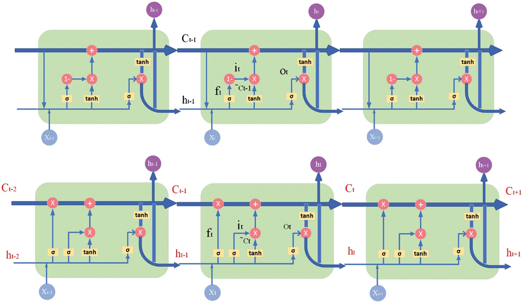
Figure 4: Improved LSTM chain structure (The top picture is before improvement, the bottom picture is after improvement)

LSTM input gate, output gate and forget gate protect and control cell state. The improved LSTM unit flows to the next unit containing the input data at the current time, the output of the hidden layer at the previous time, and the unit state from the previous time, and then the data is mapped to 0 to 1 by using the activation function (Sigmod). The expression of the forget gate is as described in formula (4).

ft=σ(Wf⋅[Ct−1,ht−1,xt]+bf)(4)

The output result of formula (5) is between 0 and 1, which represents the rate of forgetting. Then the input ratio can be constructed from this forgetting ratio. The expression of the input gate is as described in formula (5).

it=1−ft(5)

Then the new data expression for adding candidates is expressed as formula (6).

C~t=tanh(WC⋅[Ct−1,ht−1,xt]+bC)(6)

Since the input ratio and the new candidate data are known, the new unit state can be obtained, expressed as formula (7).

Ct=Ct−1+it∗C~t(7)

The input gate represents the data flowing out of all input states after transformation, expressed as formula (8).

ot=σ(W0⋅[Ct−1,ht−1,xt]+b0)(8)

Since the status of the unit and the data of the output gate have been updated, the output of the hidden layer can be obtained at this time, as described in Eq. (9).

ht=ot∗tanh(Ct)(9)

2.3 Prophet-LSTM Combined Model Construction

In order to progress the two tasks in this application scenario and perform accurate and efficient predictive analysis of high-dimensional time series data in existing datasets, this chapter constructs and proposes a P-gLSTNet fusion model. The fusion model mainly consists of three parts:

(1)   A data input module for forming a high-dimensional data flux N * T * F;

In order to clarify the structure of gLSTNet constructed in this article, the data input situation should also be clarified. The constructed high-dimensional data flux is a data cube based on multiple samples and multiple features at different moments after adding the time axis, as shown in Fig. 5. The high-dimensionality mentioned is a high-order matrix of N * T * F. The first dimension of the dimension N * T * F is the number of samples, the second dimension is time, and the third dimension is the number of features. The high-dimensional data throughput in this experiment is 90 * T under ideal conditions.

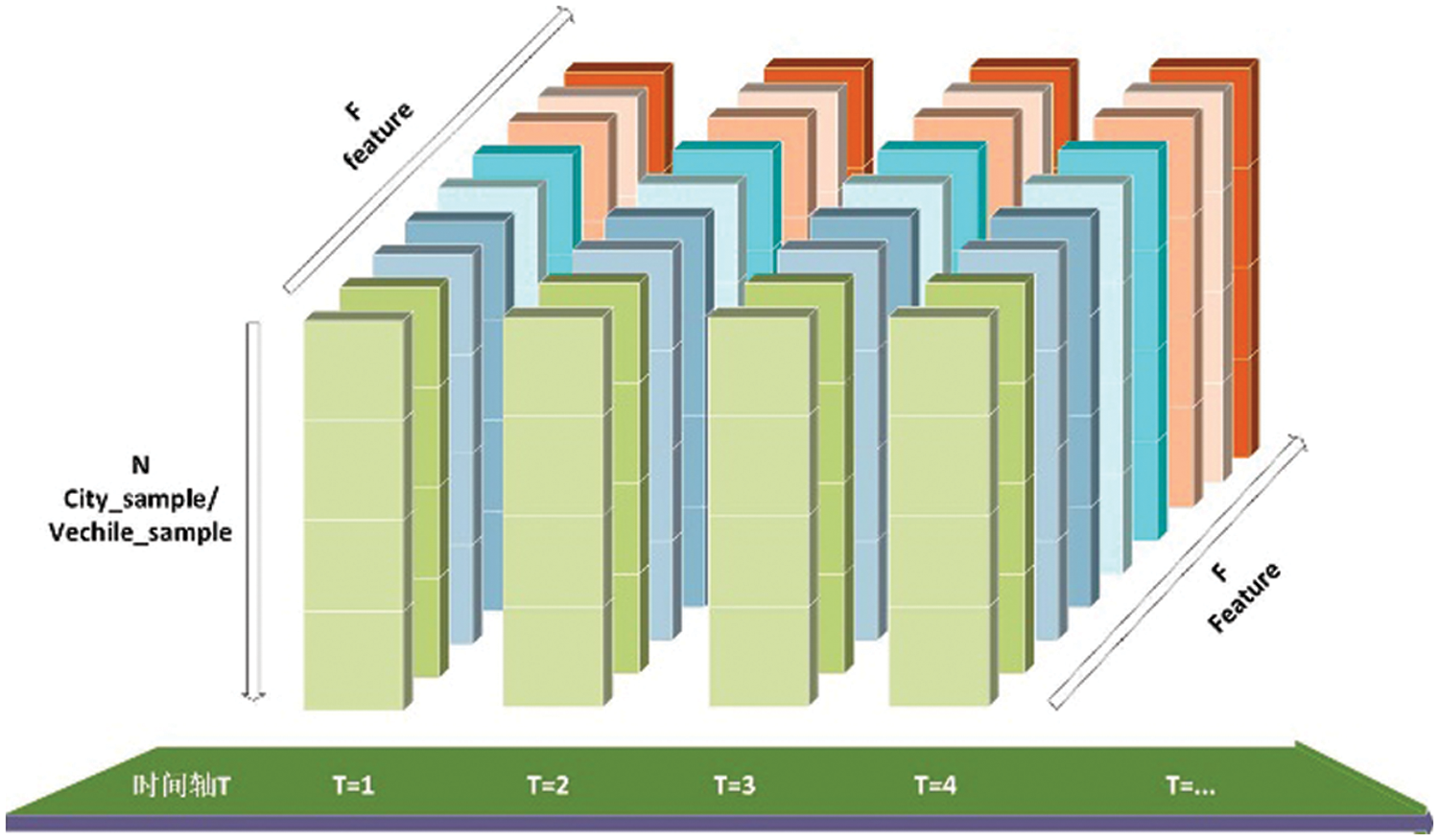
Figure 5: High-dimensional data flux feature map

(2)   gLSTNet and prophet modules trained in parallel;

The prediction model of gLSTNet constructed by the improved LSTM unit is divided into input layer, hidden layer and output layer, the model structure is shown in Fig. 6. The input layer and output layer are both set to 9-dimensional attribute input and output that conform to the characteristics of the dataset. In subsequent experiments, the 9-dimensional output plus the fully connected layer can be considered as input at the next moment. The gLSTNet constructed in this paper contains 3 hidden layers. At T = 1 and T = 2, its structure is similar to an ordinary BP network. After unfolding along the time axis, the hidden layer information H, C at the previous moment will be Transfer to the next moment, that is, the time axis transfer. Where H represents the state of the hidden layer, and C is the merged update gate. From the perspective of the network structure, the constructed gLSTNet requires high-dimensional data input and output flux. See the next section for the dimensional analysis.

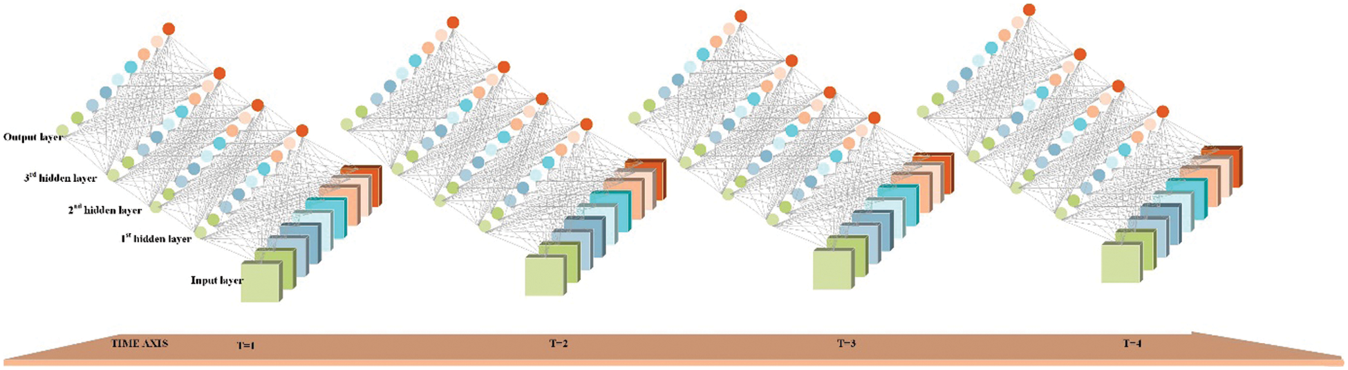
Figure 6: The gLSTNet neural network structure diagram

(3)   A module for weighted combination output based on the Particle Swarm Optimization (PSO) algorithm;

Time series data contains a lot of uncertain information, and the forecasting effect of applying a single model is often not very satisfactory [25]. Therefore, in order to improve the accuracy of prediction, the LSTM and prophet models are combined. In multiple regression, multiple linear regression analysis is performed. Common methods for solving regression parameters include least square method, gradient descent method and newton method, etc. However, these methods involve a large number of matrix calculations and the calculation speed is slow. Compared with genetic algorithm (GA) and ant colony algorithm (ACO), the PSO algorithm has the characteristics of simplicity and efficiency, fewer parameters, and faster convergence speed [11]. Therefore, this paper uses PSO algorithm to determine the weight coefficients of the combined model [26]. And the PSO algorithm is used to solve the combination coefficients of the two models to increase the speed of the solution and give full play to the advantages of the combined model.

The PSO algorithm is different from other methods of solving regression parameters. It regards the combination coefficients (α, β) as a particle, and randomly initializes multiple particles. Each particle updates the optimization equation through its own position and its own speed. The optimal solution is closer. As mentioned above, the weight is adaptively adjusted, so the weight here will change with the change of the particle fitness value. For example, formulas (10) and (11) are expressed as:

vi(k+1)=wvi(k)+c1r1(pi−xi(k))+c2r2(pg−xi(k))(10)

xi(k+1)=xi(k)+vi(k+1)(11)

Among them, vi, xi(k) are the velocity and position of the particle, respectively; c1, c2 are the acceleration terms that move to the particle’s historical optimal position pi and the current optimal position of all particles pg factor; r1, r2 are random factors between 0–1; w is the inertia factor, which is the inertia of the particle’s previous movement direction in the current movement direction.

Its overall framework is shown in Fig. 7:

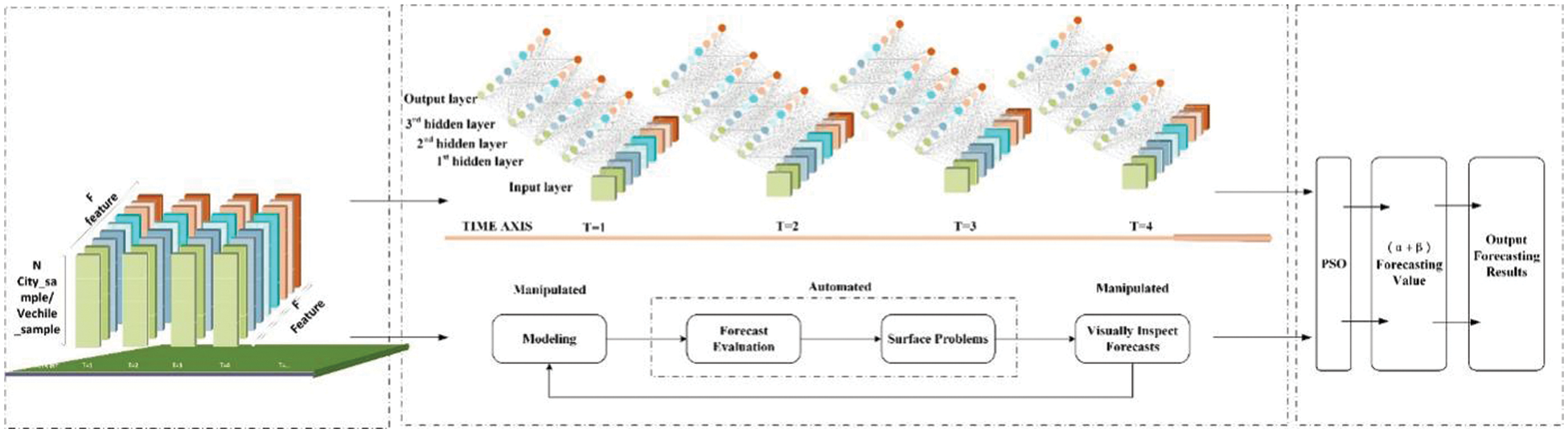
Figure 7: Schematic diagram of the structure of the P-gLSTNet fusion model

2.4 Experimental Dataset

The monitoring data of the self-collected data set comes from the high-emission vehicle installed in each actual working condition. The hardware monitoring terminal device integrated with the sensor is integrated on each vehicle. In this study, the data monitoring and analysis platform is used to realize remote monitoring, which is designed and developed on the basis of public cloud service software and hardware resources to monitor and manage the massive and multi-source non-road mobile sources generated in a fixed period. A structured database of multi-dimensional heterogeneous emission data, which forms a data resource library after preprocessing the collected monitoring data from multiple terminals. The purpose is to allow users or analysts to intuitively perceive real-time dynamic information through a large amount of data visualization, and to grasp hidden time clues through these time-series information [27].

The monitoring data comes from the integrated sensor monitoring device installed on each high-emission vehicle operating under actual working conditions. By integrating the sensor control unit, concentration acquisition module, Beidou positioning module, wireless communication module, and power management module packaged inside the sensor body, it is convenient to collect exhaust emission factors such as particles and nitrogen oxides in real time during the actual engineering operation of the vehicle. The convenience of exhaust gas monitoring is improved, and the On Board Diagnostics (OBD) reserved interface set on the upper surface of the sensor body is integrated to facilitate access to the OBD interface according to the needs of the vehicle circuit connection. The integrated sensor sends data back to the data platform every 30 s. We select the data in the time interval from 0:00:00:00 on January 1, 2021 to 23:59:59 on October 31, 2021. Through screening, a table containing 64 data is prepared for univariate time series data prediction. Each data table records the working data of one vehicle. The 64 vehicles are located in the urban or suburban areas of Beijing. The emission data can be used as a sample. A data set representing a total of 1,289,807 pieces of data in Beijing’s pollution samples was recorded as dataset1; for multivariate time series data prediction, a data table containing 10 data tables was prepared, and each data table recorded the working data of one vehicle. The cars are distributed in Bozhou, Anhui, a data set with a total of 247,244 data, denoted as dataset2.

We choose 9 monitoring features as input data, namely speed, Diesel Particulate Filter (DPF) differential pressure, DPF post pressure, DPF pre-temperature, DPF post-temperature, urea level, front NOx, rear NOx, PM. The following Fig. 8 shows an example of time series data contained in the data table in the data set, which is the time series data information of non-road mobile machinery emission of vehicle S95112 from January 1, 2021 to October 31, 2021.

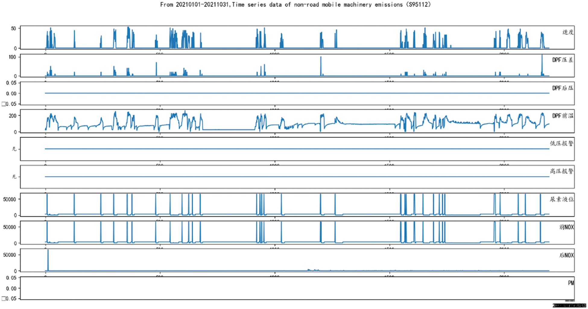
Figure 8: From January 1, 2021 to October 31, 2021, time series data of emissions from non-road mobile machinery (Vehicle S95112)

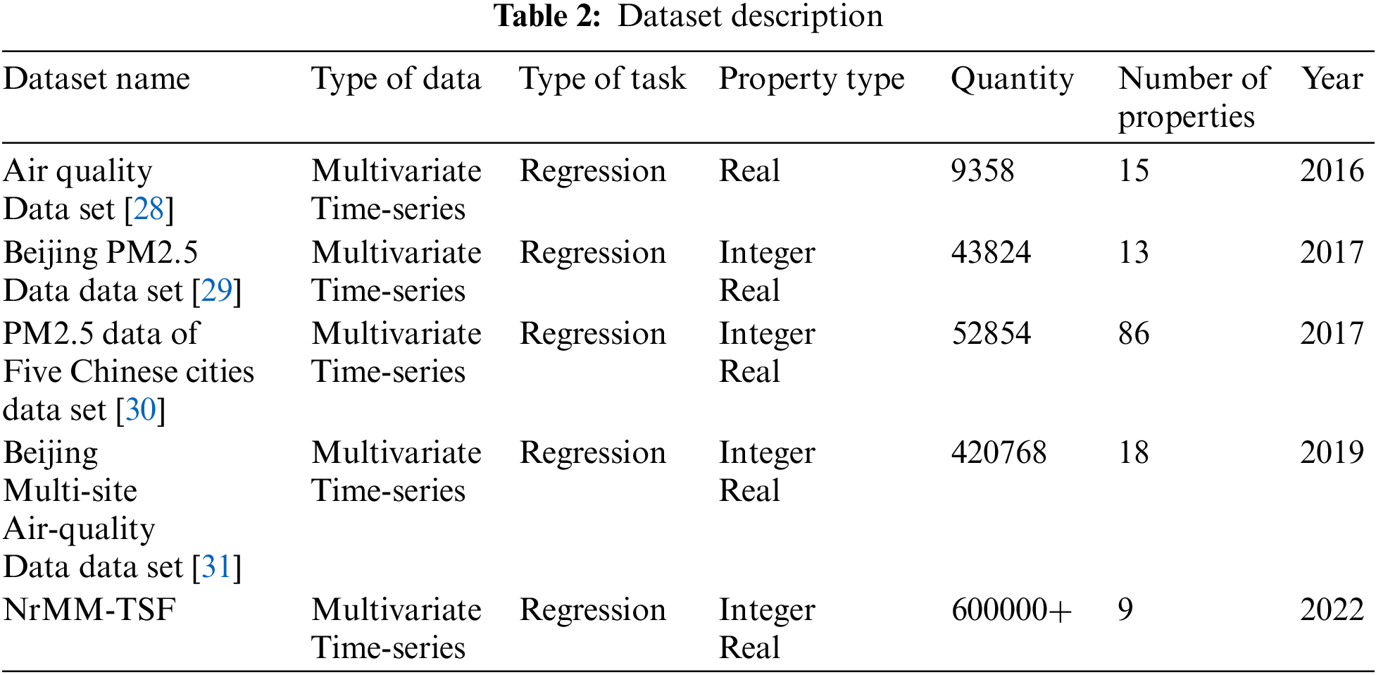
Based on the research field of this paper, this paper also selects 4 public datasets for progress experiments. The source of the dataset is the University of California, Irvine (UCI) machine learning public dataset. The details of the self-collected dataset are shown in Tab. 2. The table clarifies that the data and characteristics are weather data and pollution emission data related to air quality, all of which are multivariate time series and are suitable for multiple regression analysis tasks. The specific contents are:

(1)   The Air Quality Data Set [28] contains responses from gas multi-sensor installations deployed on-site in Italian cities, hourly response averages, and gas concentration reference records from certified analyzers.

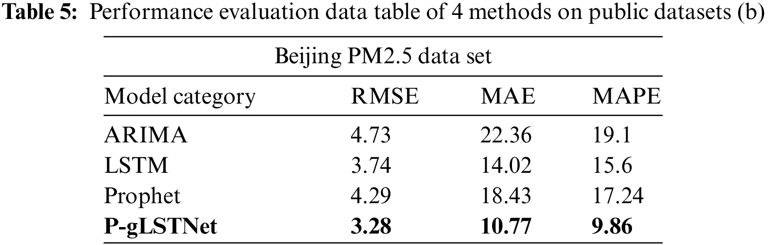
(2)   Beijing PM2.5 Data Set [29] contains hourly PM2.5 data from the US Embassy in Beijing. At the same time, it also includes the meteorological data of Beijing Capital International Airport.

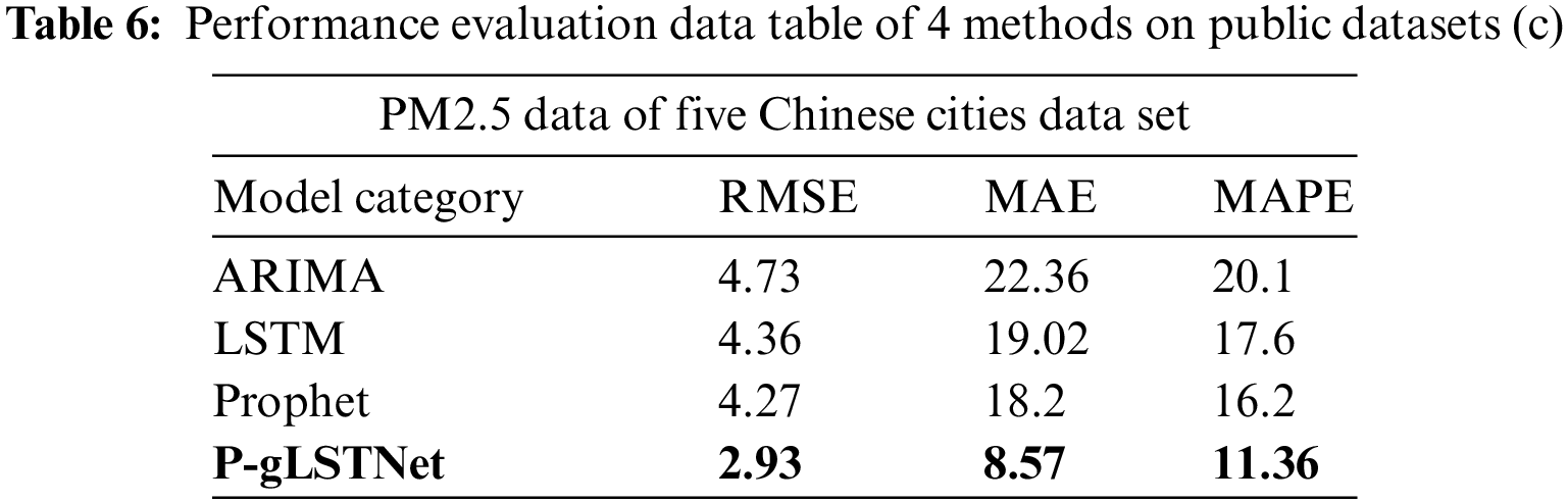
(3)   PM2.5 Data of Five Chinese Cities Data Set [30] includes hourly PM2.5 data for Beijing, Shanghai, Guangzhou, Chengdu and Shenyang; at the same time, it also includes meteorological data for each city.

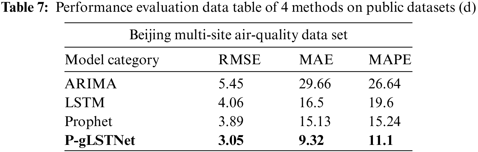
(4)   Beijing Multi-Site Air-Quality Data Set [31] contains 6 main air pollutants and 6 related meteorological variable values collected every hour at multiple sites in Beijing.

(5)   The self-collected Non-road mobile machinery exhaust emission time series forecast data (NrMM-TSF) is collected and organized by relying on the characteristics of 9 types of monitoring attributes of the subject.

3  Experiment

The key work in this section is to conduct time series prediction experiments based on four models, namely ARIMA [32], LSTM [33,34], Prophet [16] and the P-gLSTNet proposed in this article, and explain the performance indicators and parameter settings. Modeling steps based on the combined model of LSTM and Prophet:

Step 1: Use the average method to fill in the small part of the missing data in the data, combining the data trend of the past month and the data of the same period of each quarter;

Step 2: Normalize the raw data processed in step 1, so that the range of the training data is as small as possible. Then use formulas (4)–(9) to train and predict the time series {Xt} to obtain the predicted value Lt of the LSTM model;

Step 3: Log processing the raw data processed in Step 1, to make it conform to the normal distribution as much as possible. Then use Eqs. (1) to (3) to train and predict the time series {Xt}, and obtain the predicted value Pt of the Prophet model;

Step 4: By constructing the fitness function Q(θ), the predicted value of the combined model is as close to the real value as possible, and the coefficients α and β of the combined model are solved by the PSO algorithm [32];

Step 5: Combine the prediction results of the two models to obtain the combined model prediction value Xt = αLt + βPt.

The combined training parameters are set to convert the time series data into a supervised learning problem in a development environment, and apply the improved LSTM model to the training set (60%), test set (30%) and validation set (10%). Obtain various specific parameters under a single model, and set the time series data of the input vector dimension according to the forecast demand; apply prophet to the data set after log processing respectively, obtain various specific parameters under a single model, and set according to the forecast demand Set the time series data of the input vector dimension, the trend term is an improved logistic growth model, the period term is the Fourier series, and the fitting function is the Fit function.

3.1 Evaluation Index

There are various evaluation systems and evaluation indicators for time series data prediction. The simplest evaluation method is to use the image fitting degree method. The test result and the input data curve are drawn on the same data graph, and then the fitting degree of the test result and the input data curve is observed to judge. The simplicity of this method is considerable, but it is relatively general, and the objectivity of the results cannot be clearly reflected by non-numerical results. Therefore, this paper evaluates the performance of P-gLSTNet and related comparison methods by combining the three prediction evaluation indicators of mean absolute error (MAE), root mean square error (RMSE) and mean absolute percentage error (MAPE) [35].

Mean Absolute Error (MAE) is the average of all absolute errors.

MAE=1n∑i=1n|fi−yi|(12)

Root Mean Square Error is the square root of the ratio of the square of the deviation between the predicted value and the true value to the number of observations.

RMSE=1n(fi−yi)2(13)

The formula for Mean Absolute Percentage Error is as follows.

MAPE=1n∑i=1n|fi−yiyi|(14)

Among them, fi represents the prediction result, and yi represents the input data. The evaluation is carried out by calculating the average absolute error, root mean square error and relative error of multiple pairs of prediction results and input data respectively.

3.2 Parameters

3.2.1 Time Series Length and Forecast Hours

Through the analysis of the experimental data set, we can conclude that the length of the time series and forecast hours are determined by the sample target ratio. In this article, a 4:1 ratio is used [36,37]. In four different time series forecasting models, we designed four sets of experiments by changing the length of the time series. The length of the time series is chosen to be 1000 h.

3.2.2 Learning Rate

The learning rate is a hyperparameter that controls the degree to which the model is changed according to the estimated error each time the model weight is updated [38,39]. An appropriate learning rate is essential to find the optimal weights of the model [40]. The learning rate is small, the training process is long; the learning rate is large, the training process is unstable. In this paper, the initial learning rate is set to 0.01, and it is automatically adjusted during the training process. At the same time, the gradient descent Adam [41] will be used to optimize the model of part of the LSTM.

3.2.3 Parameters in P-gLSTNet Model

There are still several parameters to be determined in the model. The number of units in the module and the fully connected module represents the dimensionality of the output data. Through experiments, setting the number of neurons in the input layer to 8, the hidden layer to 1 layer, the number of neurons to 128, and the hidden layer activation function to RELU function. The activation function is the basis for the artificial neural network to extract and learn complex features [42]. These functions can bring nonlinear characteristics to the network, so that the model can adapt to various data [43]. Relu and Tanh are the two most commonly used activation functions. In general, Relu has a wider range of applications and better performance. It works best when using Relu on a fully connected layer. Model optimization is the process of using optimization algorithms to adjust hyperparameters to minimize the cost function [44,45]. A good optimization algorithm can speed up the training process and even get better results. In our experiment, the Adam algorithm with the fastest convergence rate is used. Other parameters are determined through experiments. Epoch is set to 100, 200, 500, 1000, the batch size is 10000 h, and the ratio of training set, validation set and test set is 6:3:1.

3.3 Analysis of the Result

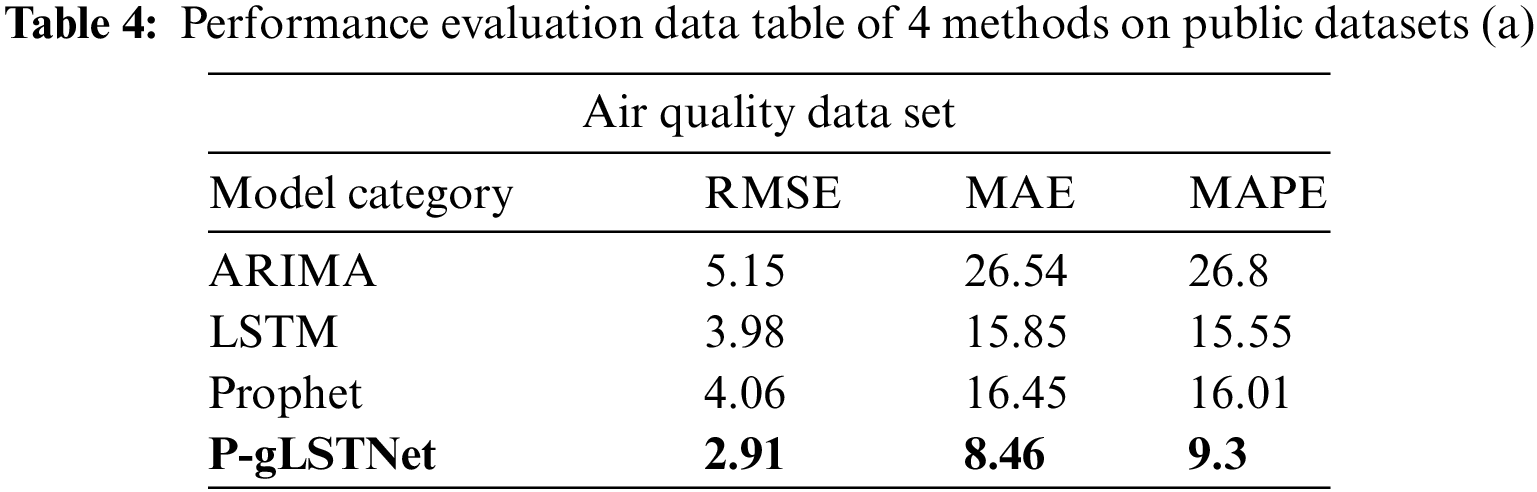
In order to prove the superiority of the model, four algorithms of ARIMA, Prophet, LSTM and fusion model P-gLSTNet are used to conduct four experiments with different time series lengths on four public datasets and one self-collected data. The prediction performance of the four methods on each dataset is shown in Tabs. 3–7.

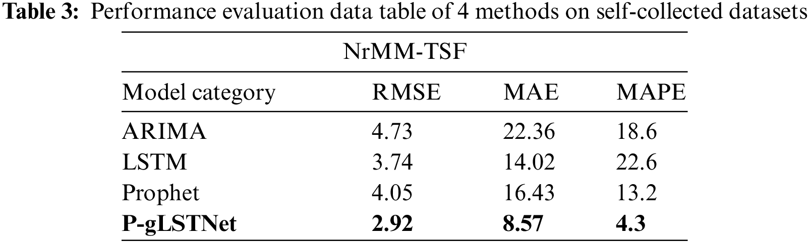
As analyzed previously, ARIMA performed the worst of the four time series prediction models when faced with multivariate and long-term dependencies. On the self-collected dataset, when the time series length processing is integrated to 1000 h, the RMSE, MAE and MAPE of the predicted results reach 4.73, 22.36 and 18.6, respectively, which are much higher than the 2.92, 8.57 and 4.3 predicted by the fusion model P-gLSTNet. The results show that, consistent with the previous studies, the traditional prediction model based on ARIMA is not suitable for time series data prediction in the fields of atmosphere and energy environment.

Compared to ARIMA’s model, the fusion model P-gLSTNet outperforms other experimental models on every metric we use, followed by LSTM and Prophet. When the time series length and prediction hours are set to 1000 h, the RMSE, MAE and MAPE values of the two backbone models reach 3.74, 14.02, 22.6 and 4.05, 16.43, 13.2, respectively, which are the best prediction results in all experiments. As the ratio of time series length to forecast hours increases, although the advantage of the fusion model P-gLSTNet gradually diminishes, it still outperforms ARIMA, LSTM and Prophet models.

Such good and bad performances are also shown on the other 4 public datasets. In order to visually display the prediction results of the model, we randomly selected the predicted value of 1000 h to compare with the actual monitoring value.

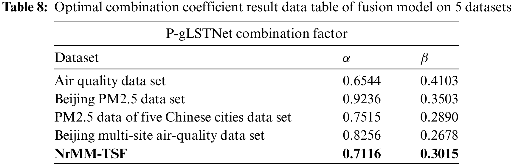
As shown in Tab. 8, based on the results of the combination coefficient solution, it is found that when the adaptive prediction reaches the optimal solution, the fusion model in this scenario accounts for the main proportion of the gLSTNet prediction results, and the Prophet model plays an important role in complementing and improving it. Combined with the weight coefficients, the optimal solution of the corresponding dataset can be given to predict the time series data P-gLSTNet, which also shows that the model can be used for migration applications under similar research. Therefore, in the next stage, it will be extended horizontally to other datasets to verify the robustness of the model.

Based on the good time series data characteristics, the pressure difference item in the multi-dimensional attribute is selected for the prediction process. The pressure difference also represents the difference between the front pressure and the back pressure of the DPF, which can characterize the working intensity of the hardware terminal equipment and facilitate the supervision of operation and maintenance. To verify the prediction accuracy of the model, you can see the comparison effect of the fitting degree, as shown in Figs. 9a–9d. Combined with data fitting and feature trends, it will play an important role in further analyzing the prediction accuracy of the fusion model and iteratively optimizing the model.

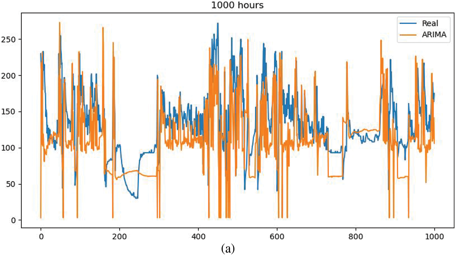
From the fitting effect of ARIMA prediction results, it can be seen that the accuracy of this method is poor. In the range of 1000 h of densely integrated data, short-term multiple fluctuations cannot be well fitted, and it cannot cope with a single long-term downward fluctuation. The reason is because the method requires that the time series data is stable, or is stable after being differentiated. In addition, the method can only capture linear relationships by nature, but not nonlinear relationships. Most of the time series data in the scene in this paper are nonlinear and do not exist in isolation. In addition, the semantic relationship between sensors needs to be explored in the next step.

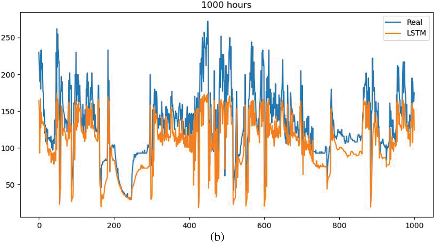
From the fitting effect of LSTM prediction results, it can be seen that the accuracy of this method is poor. In the range of 1000 h of densely integrated data, short-term multiple fluctuations can be properly fitted, and a single long-term falling fluctuation can be handled, but peaks in short-term time intervals are lost. This result shows that the use of LSTM and its variants needs to consider the appropriate time interval span, and the network is very deep, so this is also the focus of future work.

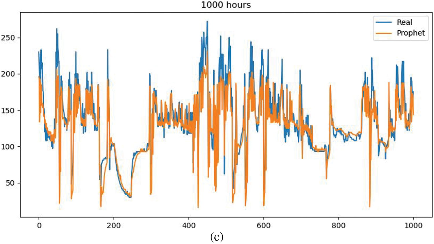
From the fitting effect of Prophet’s prediction results, it can be seen that the accuracy of this method is better. In the range of 1000 h of densely integrated data, short-term multiple fluctuations can be properly fitted, and a single long-term falling fluctuation can be well handled, but a certain amount of peaks in short-term time intervals are lost. Confirms the extensive evaluation of Prophet-efficient but imprecise, and will use this method for model checking in subsequent experiments.

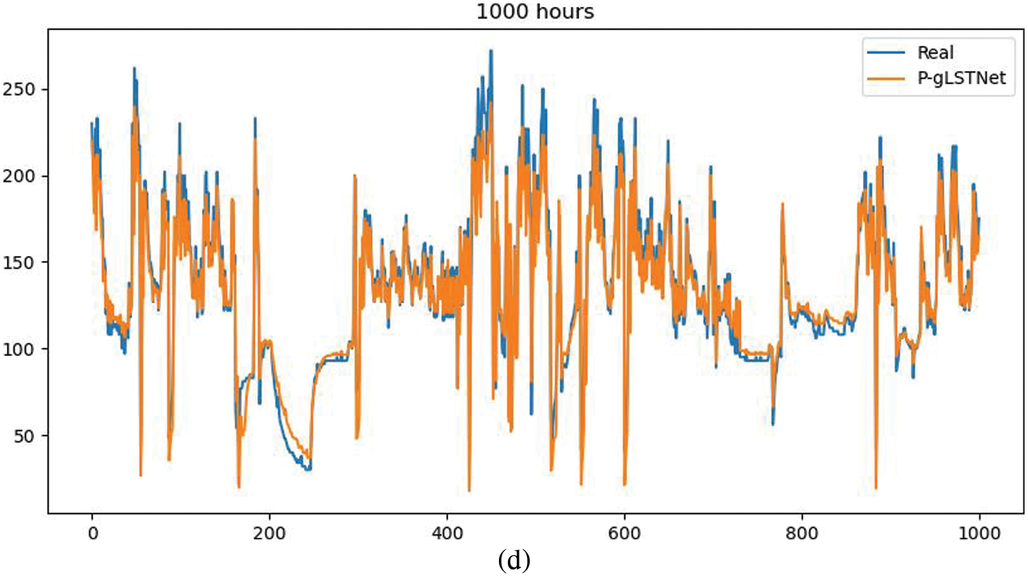
Figure 9: Comparison of actual and predicted values of the model (Vehicle S92010) (a: ARIMA, b: P-gLSTNet c: LSTM, d: Prophet)

From the fitting effect of P-gLSTNet prediction results, it can be seen that the accuracy of this method is the best among the four methods. In the range of 1000 h of densely integrated data, multiple short-term fluctuations can be properly fitted, and a single long-term downtrend can be dealt with, only missing peaks in a small number of short-term time intervals. The backbone of the P-gLSTNet model comes from the LSTM method and the Prophet method, which enables it to make full use of the advantages of the Prophet and long short-term memory networks. The model prediction accuracy is higher.

4  Conclusion

Aiming at the problem of data supervision and prediction analysis of non-road mobile source tail gas high emission, this paper studies the algorithm of time series data prediction and analysis. Based on two innovation points, theoretical research and experimental verification have been progressed:

(1)   The self-collected data set NrMM-TSF is constructed, which is the first actual data set in China under the actual working conditions of non-road mobile sources;

(2)   The fusion network model P-gLSTNet is proposed. By improving the LSTM unit and Prophet to train separately and make a weighted combination output, the two can fully pay attention to the long-term, short-interval, trend and periodic data in the scene, and it can be well adapted to the high-dimensional data throughput of the self-collected dataset NrMM-TSF in experiments.

This paper explicitly focuses on time series visualization and time series forecasting. The experiments are supported by the fusion model of the improved artificial neural network method and the traditional time series forecasting method. The experimental results serve the application scenario of high-emission vehicle exhaust pollution emission prediction and supervision. Through the analysis and mining of the periodicity, trend, data anomalies and jumping rules of the time series data set, it is possible to realize the improvement or development of air pollution control of high-emission vehicles in Beijing, Bozhou and other places for a period of time. Trend prediction can well serve the supervision and decision-making of the government and relevant environmental protection departments.

First of all, in terms of data sets, this research has made important accumulation and exploration, which is also an important innovation point. Relying on practical engineering topics, research objects such as non-road mobile machinery and high-emission vehicles that are closely related to the production and life of important domestic cities, dynamically and real-time collection of time series data sets that can be continuously maintained and enriched-Application in the fields of atmosphere, energy and environment. But the downside is that from the attribute value of the exported data table, the expected 10-dimensional attribute is not achieved. This is mainly due to the fact that many sensors under actual working conditions have not yet been connected to the central control unit to start working, resulting in the lack of data dimension. From another perspective, it can be expanded in the future.

Secondly, in terms of fusion algorithms, this research, based on the review of different time series data forecasting methods in various application scenarios, combines Prophet, LSTM model and PSO algorithm, and proposes a P-gLSTNet time series forecasting model, which can make full use of Prophet and LSTM. The advantage is that the prediction accuracy of the model is significantly improved on the basis of good response to data missing, mutation, abnormal mutation factor, seasonality and trend. The shortcoming of experimental verification is that under the multi-dimensional attribute, the training and predictive analysis are not enough, and the comparative analysis with traditional and other general or non-general models is insufficient.

In the next stage of work, we will continue to improve the comparative experiments on the LSTM variant by combining various general models or advanced algorithms, and try to introduce the attention mechanism and Transformer to improve the model; we will continue to collect and improve self-built time series datasets, and expand research, to transfer the data preprocessing method to other fields, so that the deep learning method can be better applied to the fields of atmosphere, energy and environment.

Funding Statement: This research was funded by the Beijing Chaoyang District Collaborative Innovation Project (No. CYXT2013) and the subject support of Beijing Municipal Science and Technology Key R&D Program-Capital Blue Sky Action Cultivation Project (Z19110900910000)-“Research and Demonstration of High Emission Vehicle Monitoring Equipment System Based on Sensor Integration Technology” (Z19110000911003). This work was supported by the Academic Research Projects of Beijing Union University (No. ZK80202103).

Conflicts of Interest: The authors declare that they have no conflicts of interest to report regarding the present study.

References

 1.  B. Zha, A. Vanni and Y. Hassan, “Deep transformer networks for time series classification: The NPP safety case,” 2021. [Online]. Available: https://arxiv.org/abs/2104.05448. [Google Scholar]

 2.  H. Hamdoun, A. Sagheer and H. Youness, “Energy time series forecasting-analytical and empirical assessment of conventional and machine learning models,” Journal of Intelligent and Fuzzy Systems, vol. 40, no. 2, pp. 1–26, 2021. [Google Scholar]

 3.  Y. Tang, F. Yu, W. Pedrycz, X. Yang and S. Liu, “Building trend fuzzy granulation-based LSTM recurrent neural network for long-term time series forecasting,” IEEE Transactions on Fuzzy Systems, vol. 99, pp. 1–1, 2021. [Google Scholar]

 4.  Z. K. Feng and W. J. Niu, “Hybrid artificial neural network and cooperation search algorithm for nonlinear river flow time series forecasting in humid and semi-humid regions,” Knowledge-Based Systems, vol. 211, pp. 106580, 2021. [Google Scholar]

 5.  Q. Gu and Q. Dai, “A novel active multi-source transfer learning algorithm for time series forecasting,” Applied Intelligence, vol. 51, pp. 1326–1350, 2021. [Google Scholar]

 6.  S. Bhardwaj, E. Chandrasekhar, P. Padiyar and V. M. Gadre, “A comparative study of wavelet-based ANN and classical techniques for geophysical time-series forecasting,” Computers & Geosciences, vol. 138, pp. 104461–104494, 2020. [Google Scholar]

 7.  J. Xu, Y. Hu, H. Liu, W. Mi, G. Li et al., “A novel multivariable time series prediction model for acute kidney injury in general hospitalization,” International, Journal of Medical Informatics, vol. 161, pp. 104729, 2022. [Google Scholar]

 8.  J. Monteil, A. Dekusar, C. Gambella, Y. Lassoued and M. Mevissen, “On model selection for scalable time series forecasting in transport networks,” 2021. [Online]. Available: https://arxiv.org/abs/1911.13042v3. [Google Scholar]

 9.  D. Ma, W. Ren and M. Han, “A two-stage causality method for time series prediction based on feature selection and momentary conditional independence,” Physica A: Statistical Mechanics and its Applications, vol. 595, pp. 126970, 2022. [Google Scholar]

10. I. Elvin, L. Andreas, P. Nathanael and L. Geert, “Forecasting time teries with VARMA recursions on graphs,” IEEE Transactions on Signal Processing, vol. 67, no. 18, pp. 4870–4885, 2019. [Google Scholar]

11. R. Kumar, P. Kumar and Y. Kumar, “Time series data prediction using IoT and machine learning technique,” Procedia Computer Science, vol. 167, pp. 373–381, 2020. [Google Scholar]

12. C. Satrio, W. Darmawan, B. U. Nadia and N. Hanafiah, “Time series analysis and forecasting of coronavirus disease in Indonesia using ARIMA model and PROPHET,” Procedia Computer Science, vol. 179, no. 12, pp. 524–532, 2021. [Google Scholar]

13. L. I. Yu, M. A. Ziang, Z. Pan, N. Liu and X. You, “Prophet model and Gaussian process regression-based user traffic prediction in wireless networks,” Science in China: Information Science (English Version), vol. 63, no. 4, pp. 142301:1–8, 2020. [Google Scholar]

14. D. S. D. O. Santos Júnior, J. D. Oliveira and M. De, “An intelligent hybridization of ARIMA with machine learning models for time series forecasting,” Knowledge-Based Systems, vol. 175, no. 11, pp. 72–86, 2019. [Google Scholar]

15. W. Sun, X. Chen, X. R. Zhang, G. Z. Dai, P. S. Chang et al., “A multi-feature learning model with enhanced local attention for vehicle re-identification,” Computers, Materials & Continua, vol. 69, no. 3, pp. 3549–3560, 2021. [Google Scholar]

16. G. Liang, W. Fang, Q. Zhao and X. Wang, “The hybrid PROPHET-SVR approach for forecasting product time series demand with seasonality,” Computers & Industrial Engineering, vol. 161, pp. 107598, 2021. [Google Scholar]

17. W. Sun, G. C. Zhang, X. R. Zhang, X. Zhang and N. N. Ge, “Fine-grained vehicle type classification using lightweight convolutional neural network with feature optimization and joint learning strategy,” Multimedia Tools and Applications, vol. 80, no. 20, pp. 30803–30816, 2021. [Google Scholar]

18. J. Li and Q. Dai, “A new dual weights optimization incremental learning algorithm for time series forecasting,” Applied Intelligence, vol. 49, no. 10, pp. 3668–3693, 2019. [Google Scholar]

19. C. Mcquire, K. Tilling, M. Hickman and F. De Vocht, “Forecasting the 2021 local burden of population alcohol-related harms using Bayesian structural time-series,” Addiction, vol. 114, no. 6, pp. 994–1003, 2019. [Google Scholar]

20. N. Wu, B. Green, B. Xue and S. O. Banion, “Deep transformer models for time series forecasting: The influenza prevalence case,” 2020. [Online]. Available: https://arxiv.org/abs/2001.08317. [Google Scholar]

21. R. Ye and Q. Dai, “Implementing transfer learning across different datasets for time series forecasting,” Pattern Recognition, vol. 109, pp. 107617, 2020. [Google Scholar]

22. S. K. Elsayed, A. M. Agwa, M. A. El-Dabbah and E. E. Elattar, “Slime mold optimizer for transformer parameters identification with experimental validation,” Intelligent Automation & Soft Computing, vol. 28, no. 3, pp. 639–651, 2021. [Google Scholar]

23. C. Sun, Y. Nong, Z. Chen, D. Liang, Y. Lu et al., “The ceemd-lstm-arima model and its application in time series prediction,” Journal of Physics: Conference Series, vol. 2179, no. 1, pp. 012012, 2022. [Google Scholar]

24. W. Bao, J. Yue, Y. Rao and P. Boris, “A deep learning framework for financial time series using stacked autoencoders and long-short term memory,” PLoS ONE, vol. 12, no. 7, pp. 1–24, 2017. [Google Scholar]

25. Z. Yuan, X. Li, D. Wu, X. Ban, N. Q. Wu et al., “Continuous-time prediction of industrial paste thickener system with differential ode-net,” Journal of Automation: English Edition, vol. 9, no. 4, pp. 686–698, 2022. [Google Scholar]

26. Y. Xue, A. Aouari, R. F. Mansour and S. Su, “A Hybrid Algorithm Based on PSO and GA for Feature Selection,” Journal of Cyber Security, vol. 3, no. 2, pp. 117–124, 2021. [Google Scholar]

27. X. R. Zhang, W. F. Zhang, W. Sun, X. M. Sun and S. K. Jha, “A robust 3-D medical watermarking based on wavelet transform for data protection,” Computer Systems Science & Engineering, vol. 41, no. 3, pp. 1043–1056, 2022. [Google Scholar]

28. S. De Vito, E. Massera, M. Piga, L. Martinotto and G. Di Francia, “On field calibration of an electronic nose for benzene estimation in an urban pollution monitoring scenario,” Sensors and Actuators B: Chemical, vol. 129, no. 2, pp. 750–757, 2008. [Google Scholar]

29. N. Pang, J. Gao, F. Che, T. Ma, S. Liu et al., “Cause of PM2.5 pollution during the 2016–2017 heating season in Beijing, Tianjin, and Langfang, China,” Journal of Environmental Science: English, vol. 9, pp. 201–209, 2020. [Google Scholar]

30. X. Liang, S. Li, S. Zhang, H. Huang and S. X. Chen, “PM2.5 data reliability, consistency, and air quality assessment in five Chinese cities,” Journal of Geophysical Research Atmospheres, vol. 121, no. 17, pp. 10220–10236, 2016. [Google Scholar]

31. S. Zhang, B. Guo, A. Dong, J. He, Z. Xu et al., “Cautionary tales on air-quality improvement in Beijing,” Proceedings of the Royal Society A, vol. 473, no. 2205, pp. 20170457, 2017. [Google Scholar]

32. Q. Cai, D. Zhang, Z. Wei and S. C. H. Leung, “A new fuzzy time series forecasting model combined with ant colony optimization and auto-regression,” Knowledge-Based Systems, vol. 74, pp. 61–68, 2015. [Google Scholar]

33. C. Kocak, E. Egrioglu and E. Bas, “A new deep intuitionistic fuzzy time series forecasting method based on long short-term memory,” The Journal of Supercomputing, vol. 77, no. 6, pp. 6178–6196, 2019. [Google Scholar]

34. G. Lai, W. C. Chang, Y. Yang and H. Liu, “Modeling long and short-term temporal patterns with deep neural networks,” in SIGIR ‘18: The 41st Int. ACM SIGIR Conf. on Research & Development in Information Retrieval, pp. 95–104, 2018. [Online]. Available: https://arxiv.org/pdf/1703.07015. [Google Scholar]

35. V. Cerqueira, L. Torgo and I. Mozetic, “Evaluating time series forecasting models: An empirical study on performance estimation methods,” Machine Learning, vol. 109, no. 11, pp. 1997–2028, 2020. [Google Scholar]

36. A. Ii, B. Bg, A. Mc and C. Mgb, “Explainable boosted linear regression for time series forecasting,” Pattern Recognition, vol. 120, pp. 108144, 2021. [Google Scholar]

37. W. Sun, G. Z. Dai, X. R. Zhang, X. Z. He and X. Chen, “TBE-net: A three-branch embedding network with part-aware ability and feature complementary learning for vehicle re-identification,” IEEE Transactions on Intelligent Transportation Systems, pp. 1–13, 2021. [Online]. Available: https://doi.org/10.1109/TITS.2021.3130403. [Google Scholar]

38. Y. Wang, M. H. Yang, H. Y. Zhang, X. Wu and W. X. Hu, “Data-driven prediction method for characteristics of voltage sag based on fuzzy time series,” International Journal of Electrical Power & Energy Systems, vol. 134, no. 3, pp. 107394, 2022. [Google Scholar]

39. S. C. Wen and C. H. Yang, “Time series analysis and prediction of nonlinear systems with ensemble learning framework applied to deep learning neural networks,” Information Sciences, vol. 572, pp. 167–181, 2021. [Google Scholar]

40. R. M. Farsani, E. Pazouki and J. Jecei, “A transformer self-attention model for time series forecasting,” Journal of Electrical and Computer Engineering Innovations, vol. 9, no. 1, pp. 1–10, 2021. [Google Scholar]

41. X. Shao, “Accurate multi-site daily-ahead multi-step pm2.5 concentrations forecasting using space-shared cnn-lstm,” Computers, Materials & Continua, vol. 70, no. 3, pp. 5143–5160, 2022. [Google Scholar]

42. X. R. Zhang, X. Sun, X. M. Sun, W. Sun and S. K. Jha, “Robust reversible audio watermarking scheme for telemedicine and privacy protection,” Computers, Materials & Continua, vol. 71, no. 2, pp. 3035–3050, 2022. [Google Scholar]

43. T. Liwei, F. Li, S. Yu and G. Yuankai, “Forecast of lstm-xgboost in stock price based on Bayesian optimization,” Intelligent Automation & Soft Computing, vol. 29, no. 3, pp. 855–868, 2021. [Google Scholar]

44. W. Sun, L. Dai, X. R. Zhang, P. S. Chang and X. Z. He, “RSOD: Real-time small object detection algorithm in UAV-based traffic monitoring,” in Applied Intelligence, pp. 1–16, 2021. [Online]. Available: https://doi.org/10.1007/s10489-021-02893-3. [Google Scholar]

45. H. Sun and R. Grishman, “Lexicalized dependency paths based supervised learning for relation extraction,” Computer Systems Science and Engineering, vol. 43, no. 3, pp. 861–870, 2022. [Google Scholar]