
 Submit a Paper
 Propose a Special lssue
 Open Access
ARTICLE

Salp Swarm Algorithm with Multilevel Thresholding Based Brain Tumor Segmentation Model
Computer Science Department, College of Computer Science and Information Systems, Najran University, Najran, 55461, Saudi Arabia
* Corresponding Author: Hanan T. Halawani. Email:
Computers, Materials & Continua 2023, 74(3), 6775-6788. https://doi.org/10.32604/cmc.2023.030814
Received 02 April 2022; Accepted 19 May 2022; Issue published 28 December 2022
 View Full Text
 Download PDF
Abstract
Biomedical image processing acts as an essential part of several medical applications in supporting computer aided disease diagnosis. Magnetic Resonance Image (MRI) is a commonly utilized imaging tool used to save glioma for clinical examination. Biomedical image segmentation plays a vital role in healthcare decision making process which also helps to identify the affected regions in the MRI. Though numerous segmentation models are available in the literature, it is still needed to develop effective segmentation models for BT. This study develops a salp swarm algorithm with multi-level thresholding based brain tumor segmentation (SSAMLT-BTS) model. The presented SSAMLT-BTS model initially employs bilateral filtering based on noise removal and skull stripping as a pre-processing phase. In addition, Otsu thresholding approach is applied to segment the biomedical images and the optimum threshold values are chosen by the use of SSA. Finally, active contour (AC) technique is used to identify the suspicious regions in the medical image. A comprehensive experimental analysis of the SSAMLT-BTS model is performed using benchmark dataset and the outcomes are inspected in many aspects. The simulation outcomes reported the improved outcomes of the SSAMLT-BTS model over recent approaches with maximum accuracy of 95.95%.Keywords
Brain tumor (BT) or brain cancer is a group of unusual cells from the human intelligence. There comes 2 kinds of tumors, such as benign (non-cancerous) and malignant (cancerous) [1]. Medical images are a significant means for radiologists to correctly diagnose brain diseases namely cancer [2]. High resolution MRI of the brain was required for detecting BTs in a better way. The benefit of MRI is considered the least risky technique for creating data with spatial resolution from high scale and non-invasive mode as related with other methods of diagnostic imaging. Manual segmentation of MRI pictures is time consuming, arduous, and costly and any error is vulnerable because of its indistinctness of tissues boundary, low tissue contrast, and bad hand-eye cooperation. Subsequently, dissimilarities are general amongst radiologists deciding a variability of structural forms [3]. Efficient brain MRI segmentation could probably enhance the categorization of brain diseases with better preciseness [4,5].
Histogram-related thresholding is a very famous tool from the image segmentation. Bi-level thresholding (BLT) is also termed a simple issue when compared with multi-level thresholding (MLT). Fig. 1 illustrates the process in MTL [6]. During the event of multilevel thresholding, it becomes a challenge to describe a collection of pixels if more facts of segmentation are generated. Establishing different valleys in a multi-layered histogram is not a simple job. So, the issue of multi-layered thresholding is grabbed the attention of researchers. Otsu’s technique [7], is also known as a nonparametric method, chooses optimum thresholds by increasing among-class variance of Gray level [8]. Gray levels of the picture are generally allocated the above mentioned technique is simple and robust in BLT. Otsu’s technique could probably be implemented in MLT [9]. But, it can be essentially formidable in deciding optimum thresholds owing to the exponential advances in computation time, various procedures for resolving the multi-layered thresholding issue was suggested [10]. MLT-related meta-heuristics are suggested by the researcher scholars for increasing searching speed as it has been certified to earn the optimum outcomes in (optimum) threshold.
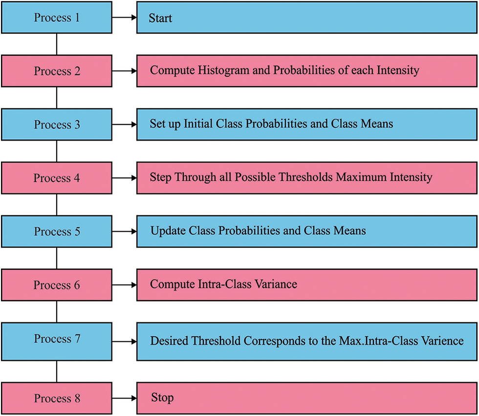
Figure 1: Process in multilevel thresholding
The authors in [11] intend to classify BTs via DL method of MR image. The UNet structure, one of the DL techniques is utilized hybrid method using pre-trained DenseNet121 structure for the classification method. In the testing and training models, the study focused on small sub-region of tumor that comprises the complicated model. In [12], an automated technique called wider residual network and pyramid pool network (WRN-PPNet) that could manually classify glioma end to end is presented. The major concept can be discussed in the following. Initially, WRN is utilized for feature extraction of multi-modal BT slices that have shown stronger expressive capability. Next, the global depiction with dissimilar levels attained through PPNet is stacked on the feature from WRN. The authors in [13] presented a multiple stage method which incorporated the domain knowledge and information into multi-sequence MR image classification. Next, we separate the presented method into, (i) visual object extraction, (ii) information modelling, and (iii) information fusion.
The authors in [14] presented an improved region-growing procedure for initializing the automated seed point. The presented technique has been compared to the advanced DL approach through the standard data set, BRATS2015. In the presented technique, the study employed a threshold method to strip the skull from all the input brain images. Next, estimated the mean intensity and the 5 blocks with maximal mean intensity have been chosen out of the 8 blocks. The authors in [15] propose a technique of augmenting a present MRI data set by producing synthetic CT image. Next, deliberate a procedure of systematic optimization of (CNN model which employs the improved data set for customizing the task. The authors in [16] introduce a level set technique viz. termed Fuzzy Kernel Level Set (FKLS) for three dimensional brain cancer classification in MR images. To evade computation difficulty, faster bounding box based symmetry analysis is utilized for extracting the volume of interest (VOI) in brain MRI. Next, a level set technique is presented on the basis of kernel mapping and fuzzy c-means clustering.
This study develops a salp swarm algorithm with multi-level thresholding based brain tumor segmentation (SSAMLT-BTS) model. The presented SSAMLT-BTS model initially employs bilateral filtering based on noise removal and skull stripping as a pre-processing phase. In addition, Otsu thresholding approach is applied to segment the biomedical images and the optimum threshold values are selected by the use of SSA. Finally, active contour (AC) technique is used to identify the suspicious regions in the medical image. A comprehensive experimental analysis of the SSAMLT-BTS model is performed using benchmark dataset and the outcomes are examined in several aspects.
In this study, a new SSAMLT-BTS model has been developed to segment BT using MRIs. The presented SSAMLT-BTS model primarily applied BF based noise removal and skull stripping as a pre-processing phase. In addition, Otsu thresholding approach is applied to segment the biomedical images and the optimum threshold values are selected by the use of SSA. Finally, AC technique is used to identify the suspicious regions in the medical image.
A primary stage, the BF technique is used to eradicate the presence of noise exist in the MRI. By combining 2 Gaussian filters, it can be able, during the domain of spatial one of which functions and intensity domain the other one is functioning. In order to weight, both the intensity as well as spatial distances were utilized. The bilateral filter outcome at pixel place p is explained as:
Whereas
Skull stripping is the preliminary step from the brain MRI segmentation method. It can be important to discard the skull in the background region from MRI for quantitative study. Generally, it can be implemented by an image filter that separates the skull and the remaining image section by covering the pixel having similar intensity level. In MR image, the skull/bone section would have a maximal threshold value (threshold > 200) than the tumour and other brain parts. Therefore, the image filter was utilized for separating the brain region according to the selected threshold value.
2.3 SSA with Otsu Thresholding Approach
Next to image pre-processing, the Otsu thresholding technique is applied for segmenation process. Otsu is the segmentation technique utilized for discovering an optimum thresholding value for the image according to the maximized between-class variance. This technique is utilized for discovering the thresholidng best value which split the images into different classifications. The approach recognizes
Now
Whereas
It is important to discover the average intensity level
Noted that
In which
Whereas
In the equation,
Now i indicates a class,
for mean value:
For optimally choosing the threshold values of the Otsu approach, the SSA is applied. SSA is determined as a random population technique suggested by [18]. It is applied to speed up the swarming technique of salps while foraging in waters. Like swarm-relied model, the position of salps can be determined in
The coefficient
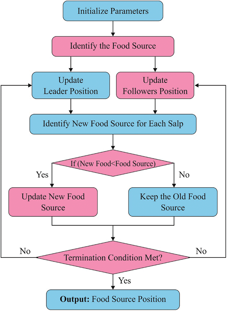
Figure 2: Flowchart of SSA
Whereas
A summary of this method is shown below:
i) Upload the parameter of SSA namely optimal fitness value
ii) Uploaded a population of S salp position in random manner.
iii) Assess the fitness of every salp.
iv) Fix amount of iteration (a) to
v) Upgraded r1.
vi) For every salp,
vii) When
viii) Then, upgraded the position of follower salp.
ix) Describe the fitness of every salp.
x) Upgraded
xi) Increment a.
xii) Follow Steps 5 to 7 until
xiii) Present the best solution
It is applied for deriving the doubtful regions from the input image. Here, the deformable snake based AC and localized AC are utilized for extracting the affected regions. It involves different processes like initialization, boundary detection, and extraction. It will track the identical set of pixels present in the pre-processed images depending on the theory of energy minimization. The energy function is defined in the following [19]:
where
where
where
In this section, a detailed experimental validation process is carried out on BRATS dataset [20]. Fig. 3 demonstrates the sample images obtained during the pre-processing stage. The first row indicates the original MRI and the pre-processed versions are offered in the second row.

Figure 3: Sample pre-processed images
Tab. 1 and Fig. 4 highlight the results offered by the SSAMLT-BTS model under different slices. On coronal slice, the SSAMLT-BTS model has offered PSNR, NCC, NAE, and SSIM of 24.65, 0.7886, 0.1935, and 93.49 dB. Moreover, on sagittal slice, the SSAMLT-BTS technique has accessible PSNR, NCC, NAE, and SSIM of 29.58, 0.8944, 0.1496, and 89.94 dB. Furthermore, on axial slice, the SSAMLT-BTS approach has obtainable PSNR, NCC, NAE, and SSIM of 31.46, 0.8579, 0.1982, and 87.74 dB.
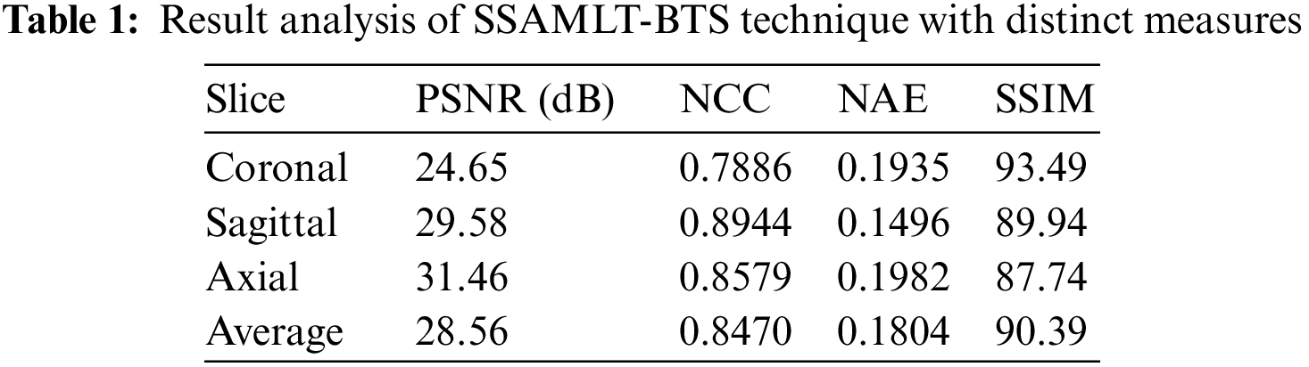
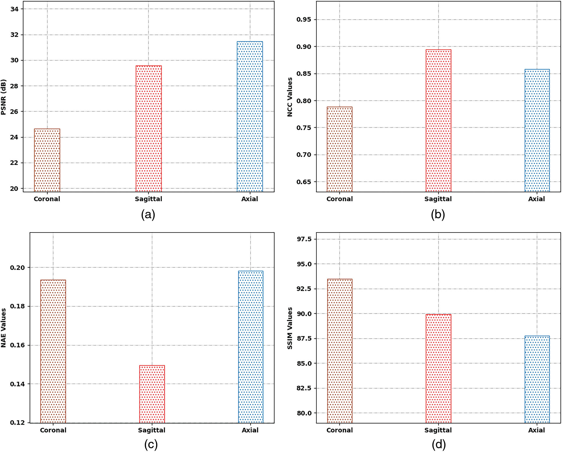
Figure 4: Result analysis of SSAMLT-BTS technique with distinct measures
Fig. 5 reports a brief average result analysis of the SSAMLT-BTS model on BT segmentation. The results indicated that the SSAMLT-BTS model has resulted in an average PSNR of 28.56 dB, NCC of 0.8470 dB, NAE of 0.1804 dB, and SSIM of 90.39 dB respectively.
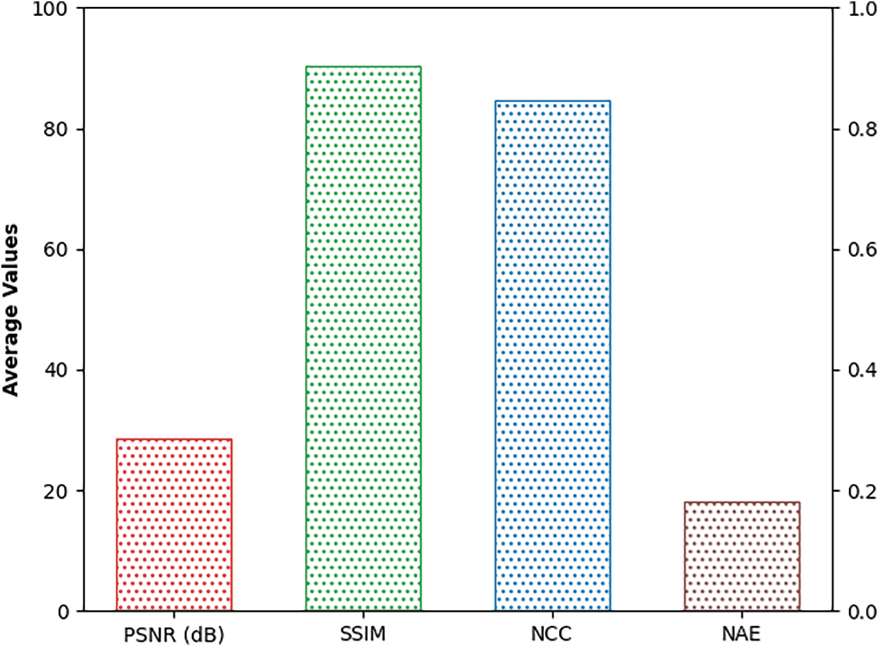
Figure 5: Average analysis of SSAMLT-BTS technique with distinct measures
Tab. 2 provides a brief result analysis of the SSAMLT-BTS model on distinct images and slice numbers. Fig. 6 reports a comprehensive Jaccard index inspection of the SSAMLT-BTS model under distinct images and slice numbers. The experimental results implied that the SSAMLT-BTS model has obtained increased values of Jaccard under all aspects. For instance, with Flair MRI image, the SSAMLT-BTS model has resulted in average Jaccard of 88.09. At the same time, with T1C MRI image, the SSAMLT-BTS model has resulted in average Jaccard of 91.46. Along with that, with T2 MRI images, the SSAMLT-BTS model has accomplished average Jaccard of 86.46.
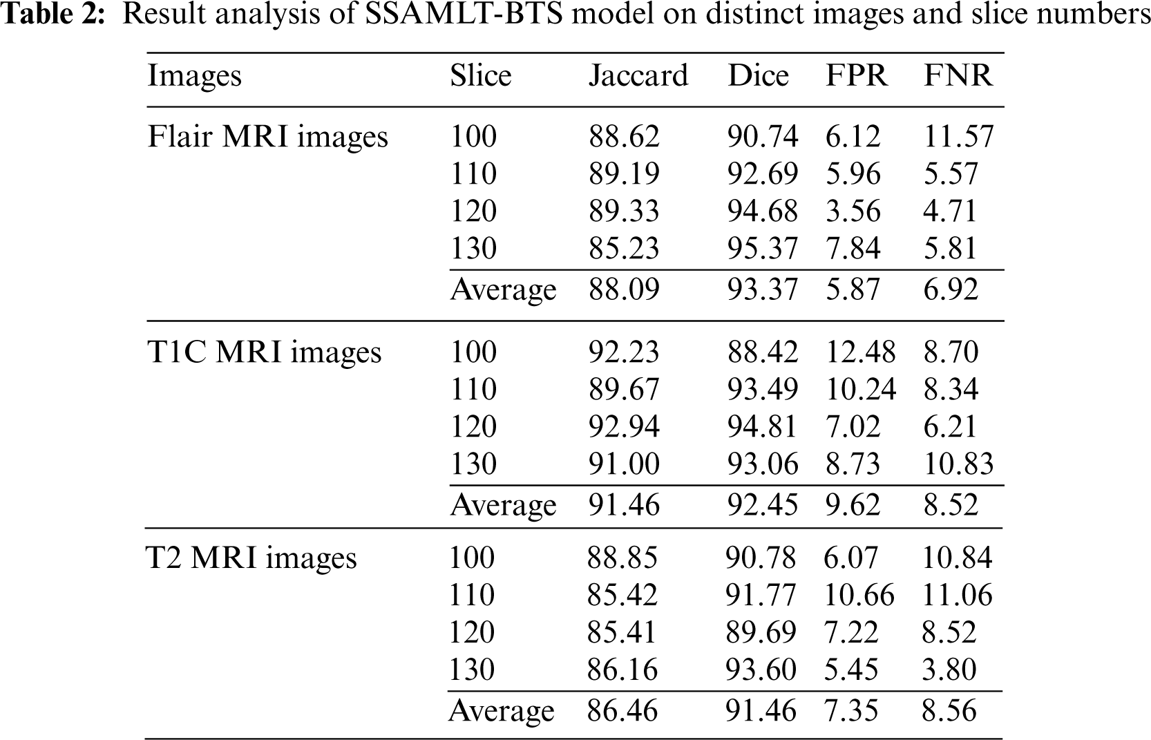
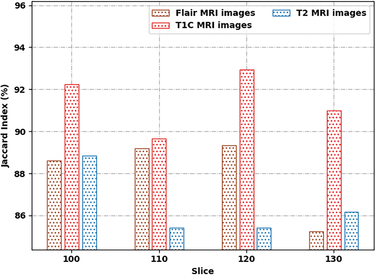
Figure 6: Jaccard index analysis of SSAMLT-BTS technique with distinct images
Fig. 7 demonstrates a comprehensive Dice inspection of the SSAMLT-BTS technique under distinct images and slice numbers. The experimental outcomes represented that the SSAMLT-BTS approach has obtained enhanced values of Dice under all aspects. For instance, with Flair MRI image, the SSAMLT-BTS methodology has resulted in average Dice of 93.37%. Simultaneously, with T1C MRI image, the SSAMLT-BTS technique has resulted in average Dice of 92.45%. Eventually, with T2 MRI image, the SSAMLT-BTS algorithm has accomplished average Dice of 91.46%.
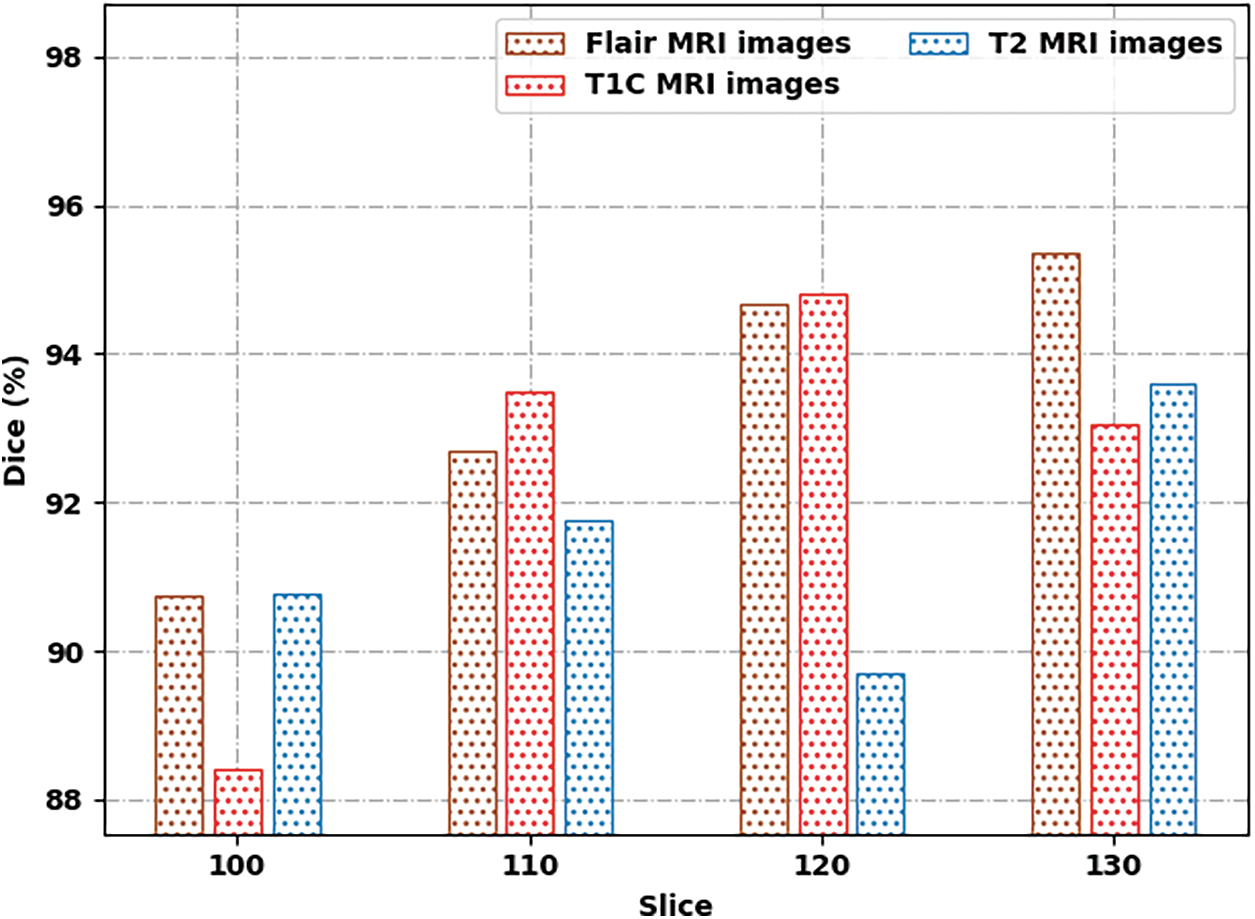
Figure 7: Dice analysis of SSAMLT-BTS technique with distinct images
At last, a comparative examination of the SSAMLT-BTS model with other models on BRATS challenges 2012 Dataset is given in Tab. 3.
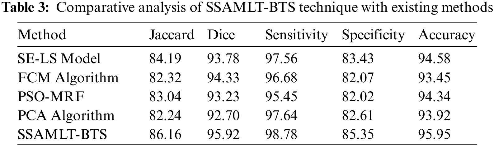
Fig. 8 reports an
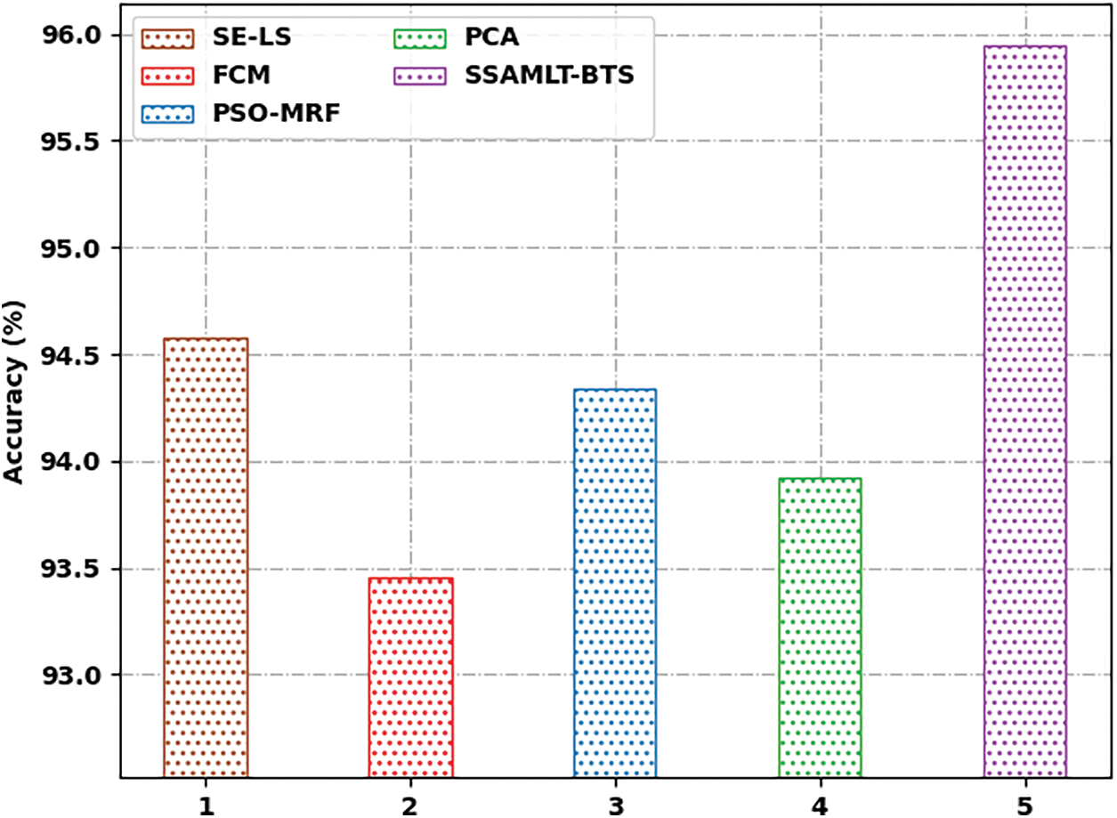
Figure 8:
Fig. 9 defines a Jaccard and Dice analysis of the SSAMLT-BTS method with other techniques. The figure exposed that the FCM and PCA models have shown worse performance with minimal values of Jaccard and Dice. Along with that, the SE-LS and PSO-MRF techniques have outperformed somewhat enhanced performance with moderate values of Jaccard and Dice. Lastly, the SSAMLT-BTS technique has accomplished superior outcomes with maximal Jaccard and Dice of 86.16% and 95.92.
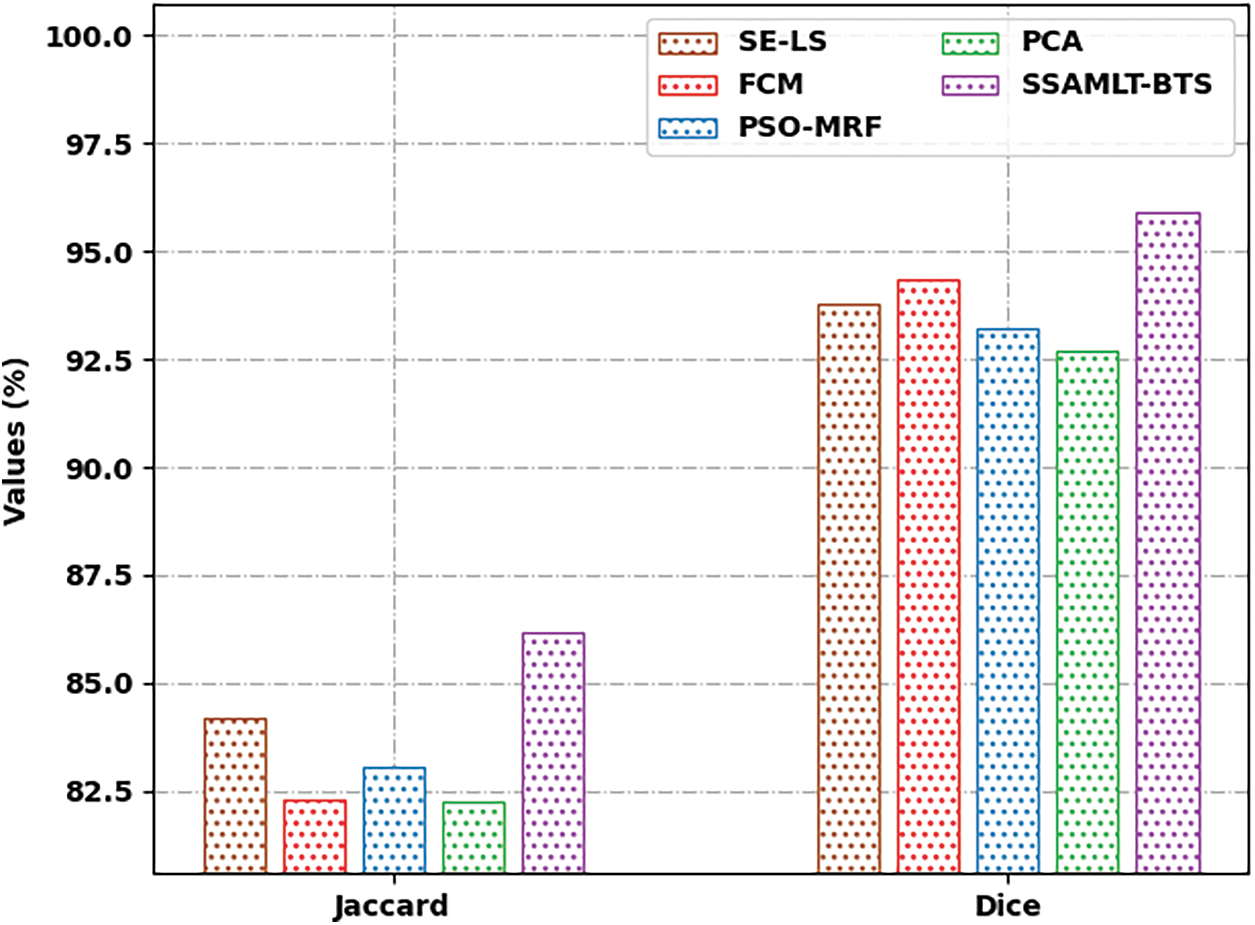
Figure 9: Jaccard and Dice analysis of SSAMLT-BTS technique with existing methodologies
Fig. 10 portrays a
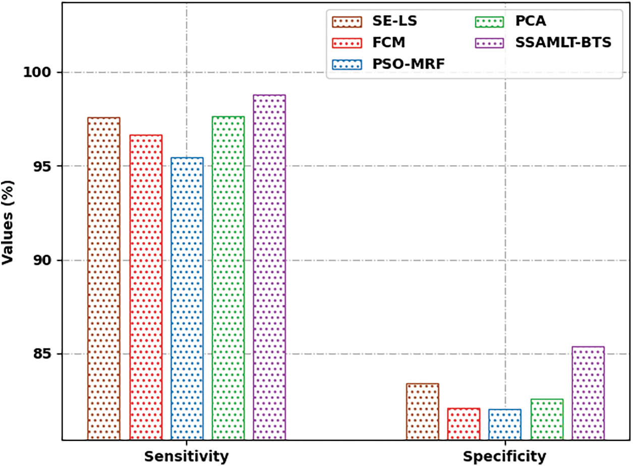
Figure 10:
In this article, an effective SSAMLT-BTS model has been introduced to identify BT using MRIs. The presented SSAMLT-BTS model primarily applied BF based noise removal and skull stripping as a pre-processing phase. In addition, Otsu thresholding approach is applied to segment the biomedical images and the optimal threshold values are selected by the use of SSA. Finally, AC technique is used to identify the suspicious regions in the medical image. A comprehensive experimental analysis of the SSAMLT-BTS model is performed using benchmark dataset and the outcomes are inspected under several aspects. The simulation outcomes reported the improved outcomes of the SSAMLT-BTS model over recent approaches. Therefore, the SSAMLT-BTS model can be applied as a proficient tool to segment MRI. In future, deep learning enabled segmentation models can be executed for improving the performance of the SSAMLT-BTS technique.
Funding Statement: The authors received no specific funding for this study.
Conflicts of Interest: The authors declare that they have no conflicts of interest to report regarding the present study.
Acknowledgment: The author would like to express their gratitude to the Ministry of Education and the Deanship of Scientific Research-Najran University-Kingdom of Saudi Arabia for their financial and technical support under code number: NU/NRP/SERC/11/3.
References
1. N. Nuechterlein and S. Mehta, “3D-ESPNet with pyramidal refinement for volumetric brain tumor image segmentation,” in Int. MICCAI Brainlesion Workshop, BrainLes 2018: Brainlesion: Glioma, Multiple Sclerosis, Stroke and Traumatic Brain Injuries, Lecture Notes in Computer Science book series, Springer, Cham, vol. 11384, pp. 245–253, 2018. [Google Scholar]
2. B. Devkota, A. Alsadoon, P. W. C. Prasad, A. K. Singh and A. Elchouemi, “Image segmentation for early stage brain tumor detection using mathematical morphological reconstruction,” Procedia Computer Science, vol. 125, pp. 115–123, 2018. [Google Scholar]
3. S. Mahajan, N. Mittal and A. K. Pandit, “Image segmentation using multilevel thresholding based on type II fuzzy entropy and marine predators algorithm,” Multimedia Tools and Applications, vol. 80, no. 13, pp. 19335–19359, 2021. [Google Scholar]
4. S. Mahajan, N. Mittal, R. Salgotra, M. Masud, H. A. Alhumyani et al., “An efficient adaptive salp swarm algorithm using type ii fuzzy entropy for multilevel thresholding image segmentation,” Computational and Mathematical Methods in Medicine, vol. 2022, pp. 1–14, 2022. [Google Scholar]
5. S. Mahajan and A. K. Pandit, “Hybrid method to supervise feature selection using signal processing and complex algebra techniques,” Multimedia Tools and Applications, 2021, https://doi.org/10.1007/s11042-021-11474-y. [Google Scholar]
6. S. Mahajan and A. K. Pandit, “Image segmentation and optimization techniques: A short overview,” Medicon Engineering Themes, vol. 2, no. 2, pp. 47–49, 2022. [Google Scholar]
7. W. Wang, X. Huang, J. Li, P. Zhang and X. Wang, “Detecting COVID-19 patients in X-ray images based on MAI-nets,” International Journal of Computational Intelligence Systems, vol. 14, no. 1, pp. 1607–1616, 2021. [Google Scholar]
8. Y. Gui and G. Zeng, “Joint learning of visual and spatial features for edit propagation from a single image,” The Visual Computer, vol. 36, no. 3, pp. 469–482, 2020. [Google Scholar]
9. W. Wang, Y. Li, T. Zou, X. Wang, J. You et al., “A novel image classification approach via dense-mobilenet models,” Mobile Information Systems, vol. 2020, pp. 1–8, 2020. [Google Scholar]
10. S. R. Zhou, J. P. Yin and J. M. Zhang, “Local binary pattern (LBP) and local phase quantization (LBQ) based on gabor filter for face representation,” Neurocomputing, vol. 116, pp. 260–264, 2013. [Google Scholar]
11. N. Cinar, A. Ozcan and M. Kaya, “A hybrid densenet121-UNet model for brain tumor segmentation from MR images,” Biomedical Signal Processing and Control, vol. 76, pp. 103647, 2022. [Google Scholar]
12. Y. Wang, C. Li, T. Zhu and J. Zhang, “Multimodal brain tumor image segmentation using WRN-PPNet,” Computerized Medical Imaging and Graphics, vol. 75, pp. 56–65, 2019. [Google Scholar]
13. K. Y. Lim and R. Mandava, “A multi-phase semi-automatic approach for multisequence brain tumor image segmentation,” Expert Systems with Applications, vol. 112, pp. 288–300, 2018. [Google Scholar]
14. E. S. Biratu, F. Schwenker, T. G. Debelee, S. R. Kebede, W. G. Negera et al., “Enhanced region growing for brain tumor mr image segmentation,” Journal of Imaging, vol. 7, no. 2, pp. 22, 2021. [Google Scholar]
15. K. T. Islam, S. Wijewickrema and S. O’Leary, “A deep learning framework for segmenting brain tumors using MRI and synthetically generated CT images,” Sensors, vol. 22, no. 2, pp. 523, 2022. [Google Scholar]
16. H. Khotanlou, O. Colliot and I. Bloch, “Automatic brain tumor segmentation using symmetry analysis and deformable models,” in Advances in Pattern Recognition, Indian Statistical Institute, Kolkata, India, pp. 198–202, 2006. [Google Scholar]
17. E. H. Houssein, M. M. Emam and A. A. Ali, “An efficient multilevel thresholding segmentation method for thermography breast cancer imaging based on improved chimp optimization algorithm,” Expert Systems with Applications, vol. 185, pp. 115651, 2021. [Google Scholar]
18. S. Mirjalili, A. H. Gandomi, S. Z. Mirjalili, S. Saremi, H. Faris et al., “Salp swarm algorithm: A bio-inspired optimizer for engineering design problems,” Advances in Engineering Software, vol. 114, pp. 163–191, 2017. [Google Scholar]
19. V. Rajinikanth, S. C. Satapathy, S. L. Fernandes and S. Nachiappan, “Entropy based segmentation of tumor from brain MR images–A study with teaching learning based optimization,” Pattern Recognition Letters, vol. 94, pp. 87–95, 2017. [Google Scholar]
20. B. H. Menze, A. Jakab, S. Bauer, J. K. Cramer, K. Farahani et al., “The multimodal brain tumor image segmentation benchmark (BRATS),” IEEE Transactions on Medical Imaging, vol. 34, no. 10, pp. 1993–2024, 2015. [Google Scholar]
Cite This Article
 Copyright © 2023 The Author(s). Published by Tech Science Press.
This work is licensed under a Creative Commons Attribution 4.0 International License , which permits unrestricted use, distribution, and reproduction in any medium, provided the original work is properly cited.
 Downloads
 Citation Tools