CE-EEN-B0: Contour Extraction Based Extended EfficientNet-B0 for Brain Tumor Classification Using MRI Images

1  Introduction

The human brain is an intricate organ made up of 50–100 billion neurons that handle the human body’s functionality. A normal healthy brain comprises of three types of tissues: white matter, grey matter, and cerebrospinal fluid. For tumor segmentation, the identification of the location is essential [1]. Due to irregular cell development inside the brain, the emergence of tumors happens. Brain tumors can be classified into three primary categories glioma, meningioma, and pituitary tumors. Gliomas are the most predominantly occurring tumors organized into high-grade gliomas (HGG) and low-grade gliomas (LGG). HGGs are malignant tumors that have fully grown. LGG is not always malignant, hence detection of LGG in an earlier stage can secure life expectancy via proper treatment [2,3]. The diagnosis of tumors includes cranial magnetic resonance imaging (MRI) and computed tomography (CT), but CT can fail to identify structural lesions, predominantly in low-grade gliomas.

The usage of MRIs is also vital in computer-aided diagnosis for rapid treatment as it provides hundreds of 2D slices with soft tissue contrast, requiring no ionizing radiation. MRI has four primary modalities, which are TI-weighted (T1w), T1w contrast-enhanced (CE), T2-weighted (T2w), and Fluid–Attenuated Inversion Recovery (FLAIR). T1 is used to distinguish between healthy tissue, and T2 is used to identify edema areas that produce a bright signal. A bright signal differentiates the T1ce from the contrast agent [2]. The Flair helps in distinguishing between edema and cerebrospinal fluid by blocking the signals of water molecules. Based on this categorization, tumors are sub-classified into tumor nuclei, reinforced tumors, and whole tumors. Tumors like Meningioma are accessible to segment, but gliomas and glioblastoma cells spread well, making it difficult to segment because they are not contrasted [1]. This segmentation between differentiating infected tumor tissues from healthy ones is achieved by classifying pixels [4]. The segmentation techniques proposed for segregation are based on the growing approach, threshold approach, watershed approach, fuzzy approach, graph-based methods, etc. [5].

The novelty of the proposed model lies in the coagulation of basic contour extraction and an extended Efficient-Net model to prepare a brain tumor classification model. The extended Efficient-Net uses some additional layers of convolution layer to extract minute features in order to classify a four-class classification problem. The contribution of the research work is as follows.

     i.  Our study presents a combination of transfer learning and image preprocessing to enhance diagnostic accuracy.

    ii.  Applying contour extraction to MRI images, extracts the particular portion of the tumor.

   iii.  The transfer learning model EfficientNetB0 has been improvised with added convolutional layers of filters 20, 40, 60 and max-pooling layers with paddings.

    iv.  This has significantly improved the overall performance of the model compared to pre-existing models.

The paper is organized in the following manner; initially, Section 2 explains the related work, followed by Section 3, comprising the dataset briefing. Section 4 provides an extensive explanation of our proposed methodology. Further, Section 5 discusses various performance measures commonly used to calculate the performance of any classifier using a confusion matrix. Section 6 exemplifies the results based on the performance classifiers. Finally, the paper concludes in Section 7.

2  Related Works

Over the past few decades, many methods of Brain tumor detection and segmentation methods have been proposed after the emergence of deep learning via convolutional neural networks [6]. Most of the classification approaches a binary way to segment between tumor and non-tumor with CNN, including convolution operation, max pooling, flattening, and fully connected layers [7]. Many non-binary classification approaches have emerged based on the location of tumors inside the brain. These include SVM (support vector machines), GoogLeNet, ANN (Artificial Neural Network), AlexNet, VGG 16, FCM, Inception V3 model, and ResNet 50 [8,9].

CNN is a multilayered, interconnected Perceptron. Commonly, CNN models consist of two layers, convolutional, and pooling layers, forming a Convolutional basis of a system. AlexNet and VGG are inculcated with Fully Connected (FC) layers [10]. In CNN classification, the convolution filter was used in the first layer, followed by reducing sensitivity in the filter by smoothing subsampling. Then the signal is transferred from one layer to another, controlled by the activation layer by fastening the training period using a Rectified Linear Unit (ReLU). Then the neurons in the proceeding layer are connected to every neuron in the subsequent layer. In the meantime, the training loss layer is added to provide feedback to the neural network [11,12]. The authors used the Jaccard similarity index to perform segmentation and claimed accuracy for 83%–95% in the segmentation of white matter, grey matter, and cerebrospinal fluid [13]. The TKFCM algorithm is an accumulation of K-means and fuzzy C-means with more minor modifications. This model obtains better results in comparison to conventional schemes. In detecting human brain tumors, the sensitivity of the proposed TKFCM algorithm is 27.07%, 4.75%, 1.98%, 2.03%, 15.11%, and 17.89% over the conventional thresholding, Region growing,’ Second-order + ANN,’ Texture Combined + ANN,’ FCM and TK mean algorithms, respectively [14].

Google launched GoogLeNet in 2014, a deep network with numerous learning layers being with two convolutional layers, two pooling, and nine inception modules. This methodology extracted features from the pooling layer, inserted after the final inception module of modified GoogLeNet. Then the features were classified applying SVM in which they had a multi-class SVM with an Error-Correcting-Output-Code (ECOC). They also used the KNN classifier in their GoogLeNet model, in which k was the number of nearest neighbors and distance metric, with five-fold validation [15]. Multiscale CNN structures are also preferred over traditional CNN structures as they reduce computational time and improve classification accuracy by proper image feature extraction of patch size identification for training [16]. The Back-Propagation neural network (BPNN) is preferred in Brain tumor segmentation with Deep Neural Networks with 2-D discrete wavelet transform and Gabor filter for feature extraction [17].

In image preprocessing, many new techniques have been developed to compress the data files. One such method is inspired by Berkeley Wavelet Transformation (BWT) and SVM as a classifier tool [18]. Principal Component Analysis (PCA) and Radial Basis Function (RBF) kernel-based SVM is used in Brain segmentation and classification, providing a similarity index of 96.20% with an overlap fraction of 95% and an extra fraction of 0.025% [19]. A medical image segmentation technique based on an active contour model to handle intensity inhomogeneity is proposed by Wang et al. [20]. A method of extreme learning machine for the classification of Brain tumors from 3D MRIs has been submitted by Deepa et al. [21]. They achieved an accuracy of 93.2% through this technique, sensitivity of 91.6%, and specificity of 97.8%.

The literature review reveals many methodologies have been designed to obtain segmentation, some for feature extraction and some for classification only. Due to the extraction of only fewer features, the resultant accuracy of tumor detection has suffered a significant reduction. The above literature also suffers a lack of calculation of similarity index, which has a significant weightage to judge the accuracy of any brain tumor segmentation algorithm.

3  Dataset

The dataset comprises a total of 3264 MRI images. The sample size of Glioma, Meningioma, Pituitary and No tumor is 926, 937, 901, and 500, respectively [22]. Fig. 1 depicts the visualization of the dataset with respect to the percentage of samples from each class. A similar dataset was used in the study by Ismael et al. [17] with a total of 3064 images consisting of Pituitary, Glioma and Meningioma Tumor MRIs which achieved an accuracy of 91.9%.

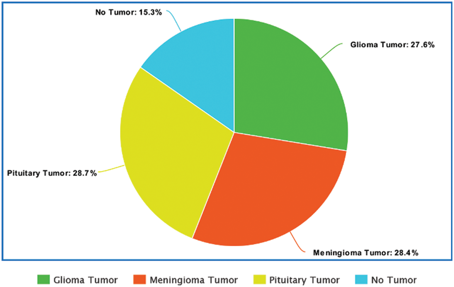
Figure 1: Visualization of the dataset

4  Proposed Methodology

Fig. 2 depicts the block diagram of the presented model involving its sub processes. Primarily, the input image is preprocessed for finding the biggest contour using contour extraction. Afterward, the extended EfficientNet-B0 model is applied to extract a valuable set of feature vectors. At last, a simple Artificial Neural Network-like structure with two Dense Layers is utilized in classification processes. Combining these three stages constitutes the Contour extraction based Extended EfficientNet-B0 model (CE-EEN-B0).

Figure 2: Steps involved in the CE-EEN-B0 model

4.1 Contour Extraction (CE): Image Pre-Processing

In our proposed methodology, we followed a preprocessing system with two significant identification stages explained in Fig. 3. The first is finding the most prominent contour that will help us distinguish the brain matter from the skull in MRIs via the convex hull technique by computing the extreme points and the Brain matter to the better approximate tumor region.

Figure 3: Steps for contour extraction

The steps for image preprocessing are defined in the following manner, and the preprocessed image outputs at every stage have been explained in Fig. 4.

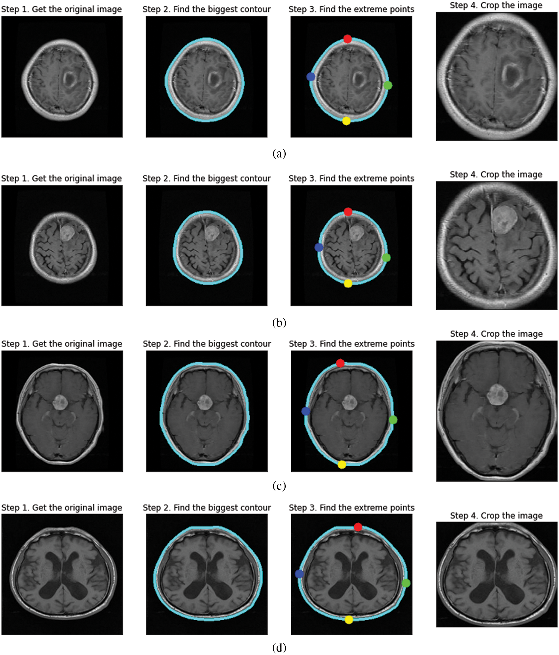
Figure 4: Contour extraction outputs for (a) glioma tumor (b) meningioma tumor (c) pituitary tumor (d) no tumor

i)   Contour is the edge boundary. To find the contours of the inputted MRI image, we call “cv2.findContours”, which is followed by sorting the contours to find the biggest one, the resultant biggest contour of brain matter is stored as a NumPy array of (x, y) coordinates.

ii)   After extracting the contour as a Numpy array, we plot the extreme points in the four directions labeled Red-North, Blue-West, Green-East, and Yellow-South. The largest and smallest x-coordinate in the NumPy array results in “West” and “East” values, respectively, similarly the largest and smallest y-coordinate in the NumPy array results in “North” and “South” values, respectively.

iii)   After plotting, the image is cropped concerning the extreme points.

Contour Extraction helps in zooming into the brain region removing the background. It helps the model to get a uniform aspect ratio of the object, that is the brain and prevents the convolution neural network to train weights specifically for zooming in or out from the image. Furthermore, it reduces the loss of information when converting to a smaller size as required in the input shape.

4.2 Extended EfficientNet-B0 (EEN-B0): Feature Extraction

An introduction to CNN networks can be found in the works of Albawi et al. [23]. A CNN network consists of many layers with filters specializing in finding a particular part of an image. CNN overcomes the challenges and performance of ANN, which simulates the way the brain analyses and processes information [24]. We have used an extended version of the transfer learning model EfficientNet-B0 with customized two-dimensional CNN layers. The approach that we use in our model here is; after the image preprocessing, we feed the output to the EfficientNet-B0 layer [25] and then pass the output from this extended layer of three Convolution Layers and Max Pooling layers, each consecutive to each other. The filters in each convolution layer are 20, 40, and 60, respectively, and the padding remains “same” in every layer. We also have reduced the learning rate when the metrics have stopped improving, as it has been found that models benefit from lowering the learning rate when learning stagnates [26]. We then pass the output to Global Average pooling and Dropout layers to prevent overfitting [27–29]. This will then be fed to the final classifier, a simple ANN Network shown in Fig. 5.

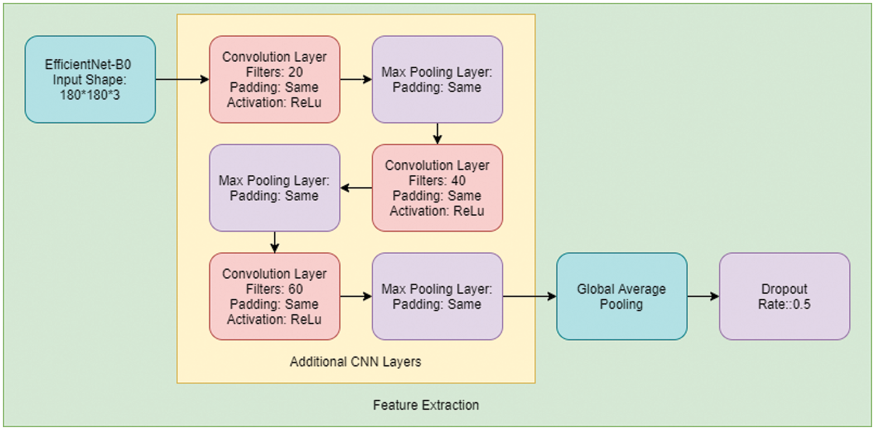
Figure 5: Working process of proposed CE-EEN-B0 model

4.2.1 Efficient Net-B0

EfficientNet is a convolutional network architecture and scaling method that balances all depth, width, and alignment equally using a compound coefficient. EfficientNet is a model group with eight models, B0–B7, and their respective performances can be seen in Fig. 6. In our model, the input shape was modified to be 180 × 180 × 3 from the default of 224 × 224 × 3. It is visible from Tan and Le that EfficientNet fared better than other Transfer Learning models. EfficientNet in recent times has been used in many machine learning classifications. Marques et al. have used it to diagnose COVID-19, getting an accuracy of 99.62% for binary classification [30]. Therefore, the Efficient-Net is selected as it provides a good starting point due to its robustness and good performance metrics.

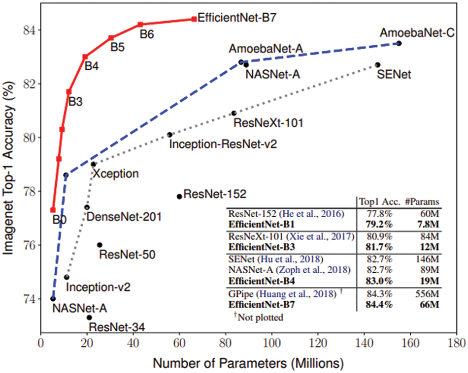
Figure 6: Comparison of models

4.2.2 Convolution Layers

The convolution layers are basic building blocks of Convolution Neural Networks. The simplest form to declare a convolution layer is:

keras.layers.Conv2D (filters = 20, kernel_size = (3, 3), padding = ‘same’, activation = ‘relu’)

The function’s many more arguments can be used; this is the official documentation for reference [31]. The filters argument determines the total number of output filters, and kernel_size is a tuple/list that determines the size of the 2D convolution window. The filters slide through the entire image matrix to find a match.

4.2.3 Activation Function for Feature Extraction Layer

ReLU, sigmoid, tanh, exponential, softmax are some of the activation functions built into Keras. The activation function that we use in our additional layers is ReLU. ReLU is generally preferred in the mid-layers of a neural network as it solves the vanishing gradients problem that is seen when using the sigmoid or tanh functions in the hidden layers of a CNN. Furthermore, it is more computationally efficient compared to sigmoid functions and it shows better convergence performance.

The ReLU activation function returns 0 if the input is less than 0 and returns x if the input is greater than 0, visualized in Fig. 7.

ReLU:f(x)=max(0,x)(1)

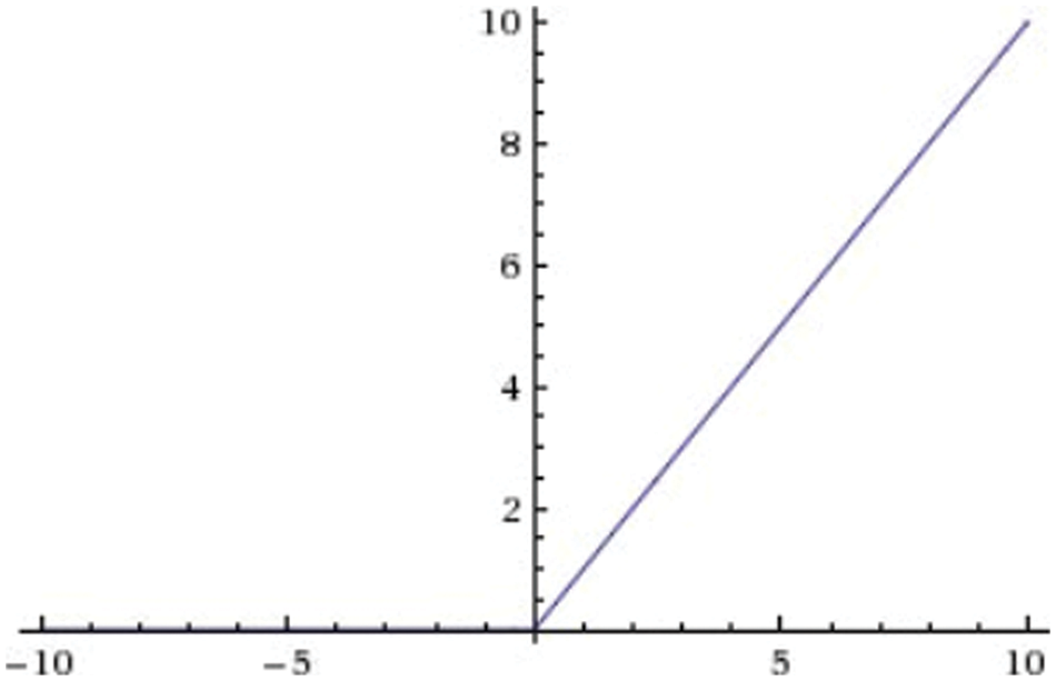
Figure 7: ReLU function

4.2.4 Reduce Learning Rate on Plateau and Saving the Best Fit Model

The model’s learning rate was reduced when the validation accuracy did not change much and the optimal model parameters and weights were saved by monitoring the validation accuracy. The optimal weights were saved in the 37th epoch while training the model with all the training images.

The criteria for reducing the learning rate was if the validation accuracy did not change by a minimum of 0.1% for 2 epochs we change the learning rate by a factor of 0.3,

New Learning Rate=Learning Rate×0.3(2)

4.3 Classification

A simple Artificial Neural network-like structure controls the classification in Fig. 8, with two dense layers with 128 and 4 units. The first layer has an activation function of ReLU, and the final classification layer has an activation function of softmax.

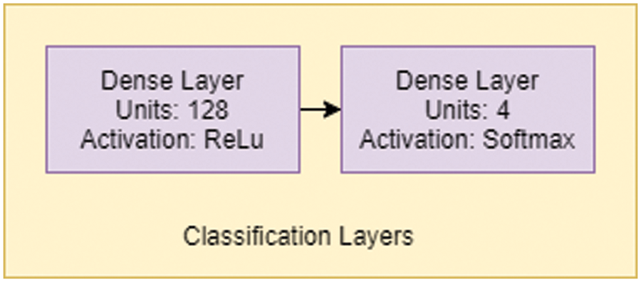
Figure 8: Classification layer

4.3.1 Activation Function for Classification Layer

The first dense layer is controlled by the ReLU function like the convolution layers before it, whereas the softmax function activates the second layer. The softmax function is defined as below where σ is softmax, z→ is the input vector, ezi is a standard exponential function for an input vector, K is the number of classes in the multi-class classifier, and ezj is a standard exponential function for output vector.

σ(z→)i=ezi∑j=1Kezj(3)

4.3.2 Loss Function

Feature Extraction and classification are part of the same model, so they share the same loss function. Categorical Cross Entropy is used as the loss function when the classification is one-hot encoded. The function is defined in Eq. (3).

CCE(p,t)=−∑n=1n(to,nlog⁡po,n)(4)

Here, t = the target value, p = the predicted value. Similarly, Sparse Categorical Cross Entropy is used majorly when the classes are mutually exclusive, i.e., glioma tumor, pituitary tumor, meningioma tumor, and no tumor and they are not one-hot encoded.

5  Performance Measures

A confusion matrix is a tabular summary of the classifier’s number of correct and incorrect predictions. It is used to analyse the performance of the classification model. The terminologies used for classifications are true positive, true negative, false positivite, and false negative. True positives is defined as the number of positive examples which are correctly classified as positive. True negatives can be defined as the number of negative examples correctly classified as negative; false positives are the number of negative examples wrongly classified as positive. False negatives are the number of positive examples wrongly classified as negative. The most importantly used performance matrices derived from the confusion matrix are accuracy, precision, recall, and F1-score. Accuracy is the ratio of all the correctly classified samples to the total number of test samples shown in Eq. (4). Precision (also called positive predictive value) is defined as the ratio of true positive to the total positive instances detected by the model as shown in Eq. (5). Recall is defined as the ratio of true positive to the summation of true positive and false negative as shown in Eq. (6). F1 score and can be described as the harmonic mean of the precision and recall as shown in Eq. (7). K-fold cross-validation is a method used in averaging out the classifier’s performance by repetitively operating on a different set of training and testing datasets of the original dataset. In this model, we performed a five-fold cross-validation technique [32].

Accuracy=TN+TPTN+TP+FN+FP(5)

Precision=TPTP+FP(6)

Recall=TPTP+FN(7)

F1score=2×Precision×RecallPrecision+Recall(8)

6  Results and Discussions

6.1 Training Result Analysis

From Fig. 9, it is observable that the training accuracy in the first fold reaches close to 99% within 12 epochs. The training accuracies from the second fold onwards maintains the 99% mark starting from the 1st epoch. These observations are for both with and without CE stage as shown in Figs. 9a and 9b respectively. From the confusion matrix in Table 1, it is detected that the False Negatives (FN), False Positives (FP) and True Negative (TN) rates being null for all the classes except Meningioma Tumor, in which one image was misclassified as Pituitary Tumor. From the confusion matrix in Table 2, it is inferred that the False Negatives (FN), False Positives (FP), and True Negative (TN) rates being null for all the classes.

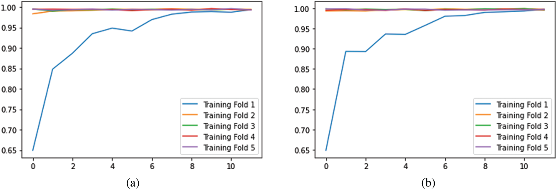
Figure 9: Visualization of accuracies vs. epochs in training analysis (a) without CE (b) with CE

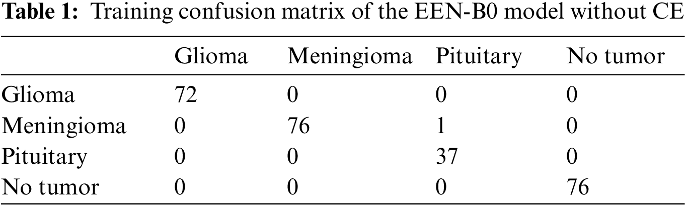
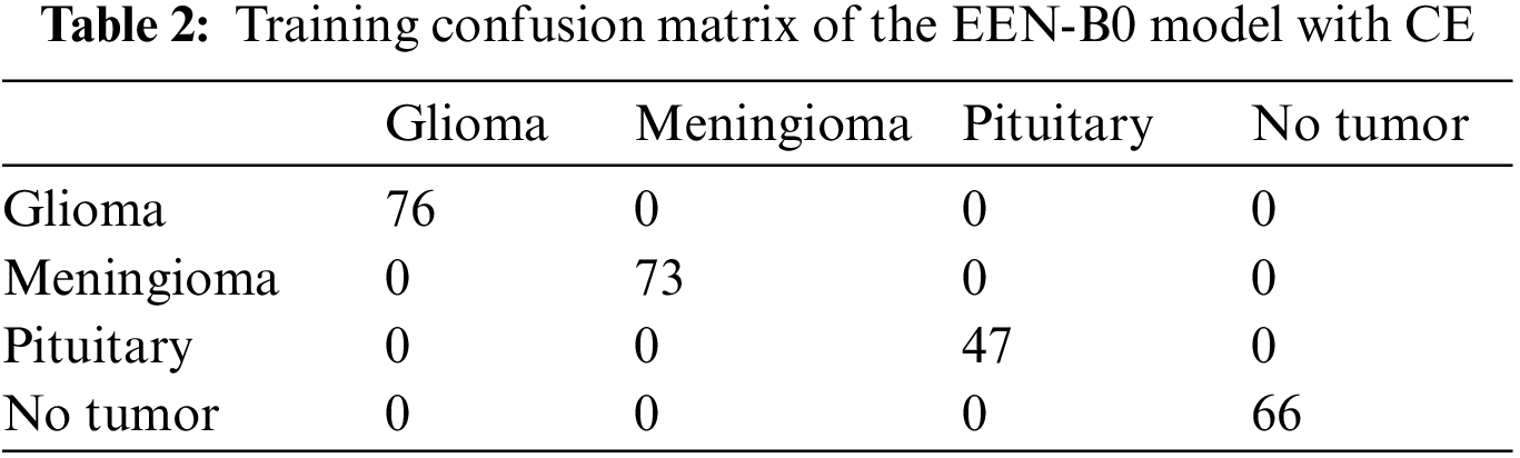
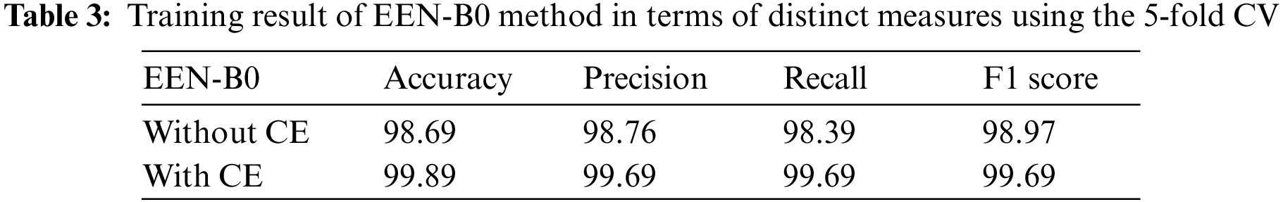
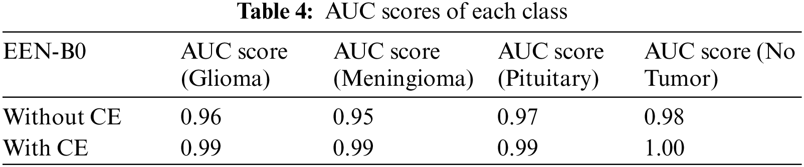
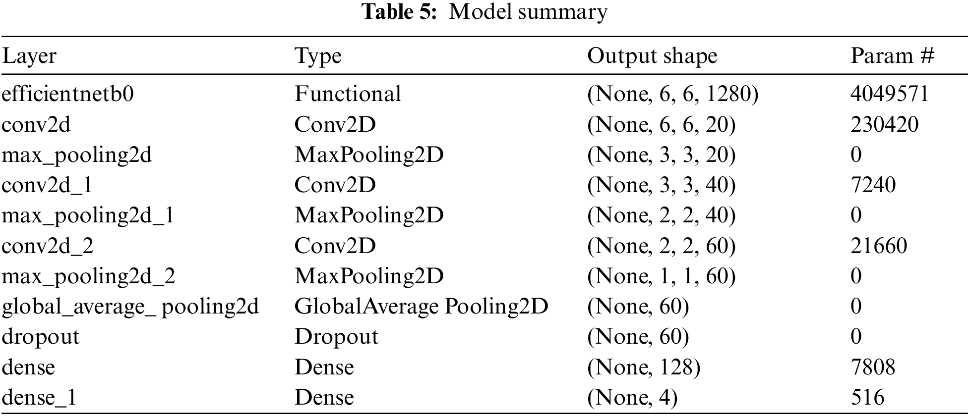
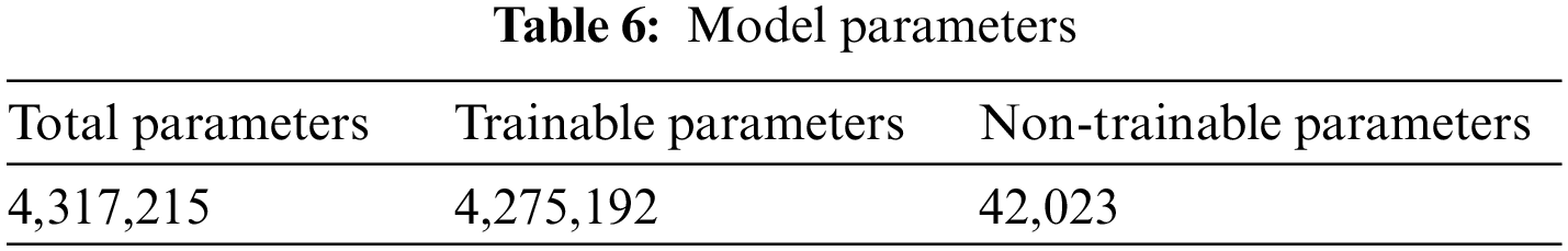
Table 3 summarizes the training result analysis of the proposed model in terms of distinct evaluation parameters. On looking into the table, it is observed that the training analysis of the model without contour extraction (CE) has led to a precision value of 98.76%, recall value of 98.39%, F1-score of 98.97%, and an accuracy of 98.69%. In addition, the training analysis of the model with image preprocessing has a slightly better performance than the model without image preprocessing with certainly higher precision value, recall value, f1-score, and an accuracy of 99.69%, 99.69%, 99.69%, and 99.89%, respectively. From the results, it is visible that the model with image preprocessing is performing prominently better. Table 4 summarizes the AUC Scores of Glioma, Meningioma, Pituitary, and No Tumor to be 0.96, 0.95, 0.97, 0.98 without CE and 0.99, 0.99, 0.99, 1 with CE. It is visible that the AUC scores of the model with CE are better. Table 5 summarizes the model and the total number of parameters per layer in the model. Table 6 denotes the total number of parameters in the model, that is; 4,317,215 and the total number of trainable parameters; 4,275,192.

From Fig. 10, it is observed that the classifier can correctly distinguish between all the positive and negative class points since the AUC value equals 1 for all the four classes in both with and without CE models as shown in Figs. 10a and 10b respectively.

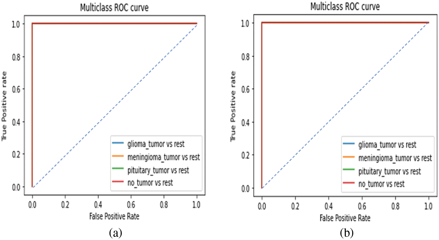
Figure 10: ROC curve for the proposed EEN-B0 model (a) without CE (b) with CE

6.2 Testing Result Analysis

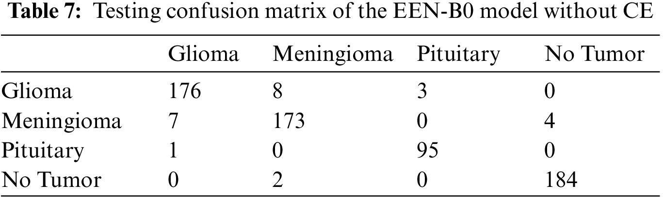
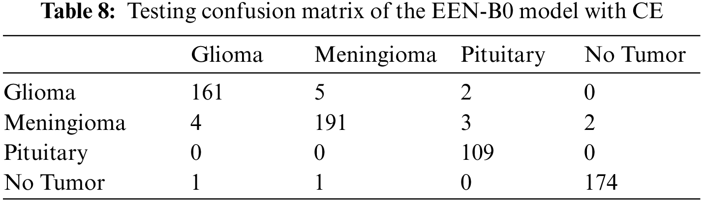
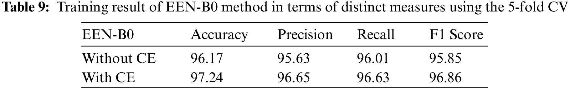
From the confusion matrix in Tables 7 and 8, it is understood that true positive (TP) rates of all the four classes are high. Glioma tumor classifies 176 out of its 184 images, Meningioma tumor classifies 173 out of its 183 images, Pituitary tumor classifies 95 out of its 98 images, No tumor classifies 184 out of its 188 images precisely in the model without CE. Whereas, in the model with CE, Glioma tumor classifies 161 out of its 166 images, Meningioma tumor classifies 191 out of its 197 images, Pituitary tumor classifies 109 out of its 114 images, No tumor classifies 174 out of its 176 images precisely. Though the given dataset is not balanced, yet as evidenced by the test results where we split the dataset in 80:20 training and testing sets, there is negligible bias for the images and does not affect the process of classification. Also, the precision and recall values which are on the higher side infer that there is no evident impact of the imbalance on the model. Table 9 summarizes the testing result analysis of the proposed model in terms of distinct evaluation parameters. On observing the table, it is concluded that the model’s testing analysis without CE has led to a precision value of 95.63%, recall value of 96.01%, F1-score of 95.85%, and an accuracy of 96.17%. In addition, the testing analysis of the model with CE has surpassed the model without CE with certainly higher precision value, recall value, f1-score, and an accuracy of 96.65%, 96.63%, 96.86%, 97.24%, respectively. It is evident from the following analysis that contour extraction based extended EfficientNet-B0 (CE-EEN-B0) performs better.

6.3 Comparative Result Analysis with Existing Models

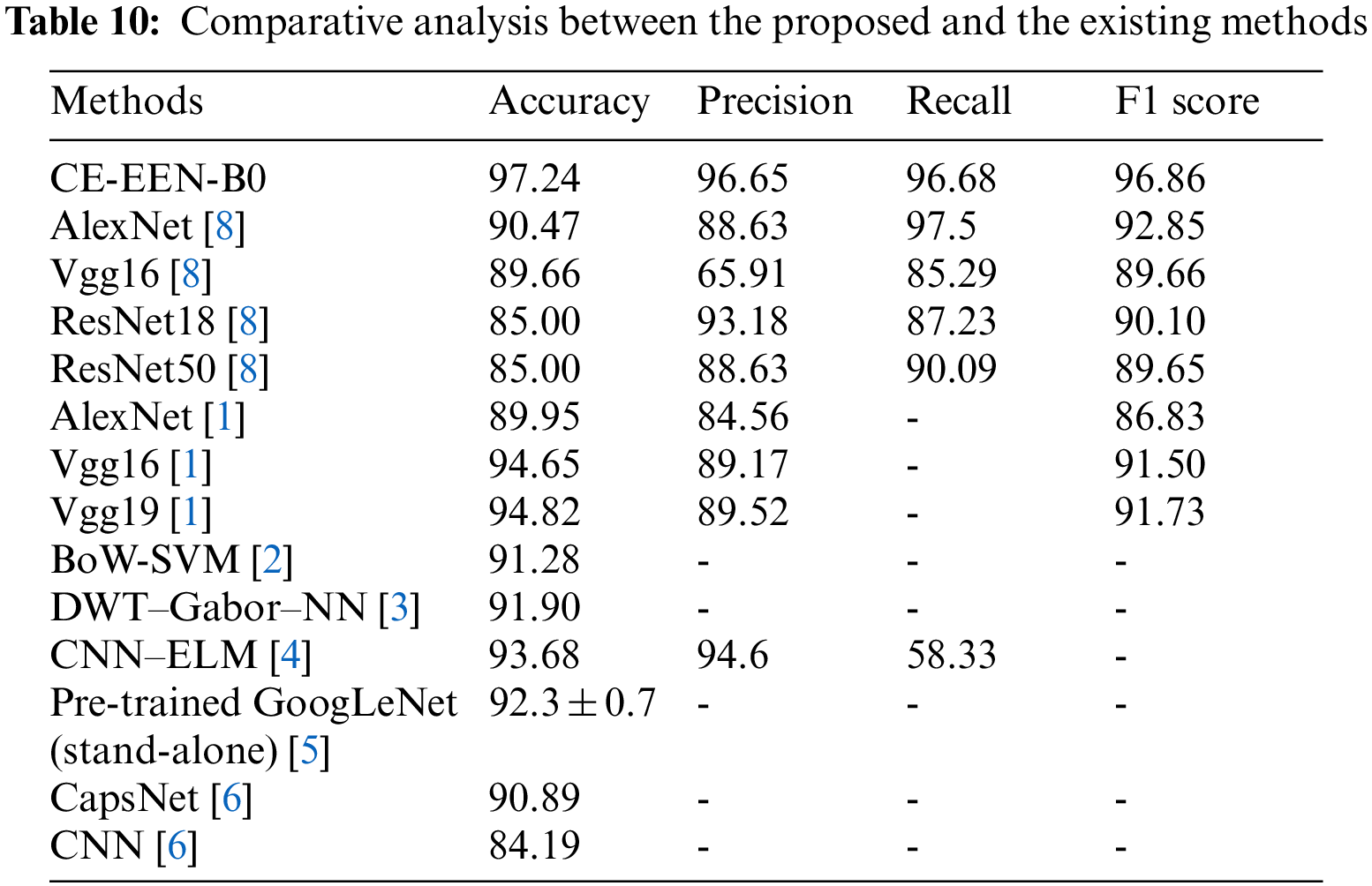
Table 10 implies the analysis of the comparative results of the EfficientNet B0 method with previous approaches through various metrics. The experimental outcome means that the proposed contour extraction based extended EfficientNet-B0 (CE-EEN-B0) model has shown a testing accuracy of 97.24%, F1-score of 96.86%, and precision of 96.65%, which significantly outperformed other existing models used for brain tumor classification.

The computational complexity for the proposed methodology is calculated by analysing the number of training samples (N) along with the feature extraction model and CNN architecture. The feature extraction model has a time complexity of O(N). The time complexity of the CNN architecture depends on the training time with all the hyper parameter values fixed throughout the process which makes it be O(N). So, finally, the time complexity of the overall model is O(N).

7  Conclusion

In this paper, a CNN architecture comprising an enhanced image pre-processing technique is proposed. This methodology tries to ease the complicated technique of brain tumor classification with a new approach based on fine-tuned transfer learning. The proposed method requires minimalistic image preprocessing for 2-D MRI images that do not require handcrafted features compared to classical systems. The proposed method of contour extraction based on extended EfficientNet-B0 (CE-EEN-B0) has outperformed state-of-the-art traditional machine learning methods and beat the state-of-the-art CNNs process on a similar dataset. The model helps classify four different types of brain tumors i.e., Pituitary tumors, Meningioma tumors, and Glioma tumors or no tumors. Though the results seem promising using the proposed model, EfficientNet is computationally heavy and needs a good processor for training purposes. The future work will be focused on running the model on a system with GPU-enabled capability to reduce computationally overhead, which can help explore better fine-tuning strategies.

Acknowledgement: The authors would like to thank the School of Computer Science and Engineering, and the Centre for Cyber Physical Systems Vellore Institute of Technology, Chennai for their constant support and motivation to carry out this research.

Funding Statement: The author(s) received no specific funding for this study.

Conflicts of Interest: The authors declare that they have no conflicts of interest to report regarding the present study.

References

1. M. Havaei, A. Davy, D. Warde-Farley, A. Biard, A. Courville et al., “Brain tumor segmentation with deep neural networks,” Medical Image Analysis, vol. 35, no. 1, pp. 18–31, 2017. [Google Scholar]
2. L. M. DeAngelis, “Brain tumors,” The New England Journal of Medicine, vol. 344, no. 2, pp. 114–123, 2001. [Google Scholar]
3. M. U. Rehman, S. Cho, J. Kim and K. T. Chong, “BrainSeg-Net: Brain tumor mr image segmentation via enhanced encoder–decoder network,” Diagnostics, vol. 11, no. 2, pp. 169, 2021. [Google Scholar]
4. G. Litjens, T. Kooi, B. E. Bejnordi, A. Setio, F. Ciompi et al., “A survey on deep learning in medical image analysis,” Medical Image Analysis, vol. 42, no. 1, pp. 60–88, 2017. [Google Scholar]
5. A. Aslam, E. Khan and M. M. S. Beg, “Improved edge detection algorithm for brain tumor segmentation,” Procedia Computer Science, vol. 58, no. 1, pp. 430–437, 2015. [Google Scholar]
6. M. D. Zeiler and R. Fergus, “Visualizing and understanding convolutional networks,” in Proc. Computer Vision–ECCV, Zurich, Switzerland, vol. 8689, no. 1, pp. 818–833, 2014. [Google Scholar]
7. N. Saranya, D. Karthika Renuka and J. N. Kanthan, “Brain tumor classification using convolution neural network,” Journal of Physics Conference Series, vol. 1916, no. 1, pp. 012206, 2021. [Google Scholar]
8. S. M. Kulkarni and G. Sundari, “A framework for brain tumor segmentation and classification using deep learning algorithm,” International Journal of Advance Computer Science Application, vol. 11, no. 8, pp. 1–9, 2020. [Google Scholar]
9. M. Sajjad, S. Khan, K. Muhammad, W. Wu, A. Ullah et al., “Multi-grade brain tumor classification using deep cnn with extensive data augmentation,” Journal of Computer Science, vol. 30, pp. 174–182, 2019. [Google Scholar]
10. R. A. Kirithika and E. Al, “An efficient ensemble of brain tumour segmentation and classification using machine learning and deep learning based inception networks,” Turkish Journal of Computer and Mathematics Education, vol. 12, no. 2, pp. 1–12, 2021. [Google Scholar]
11. J. Seetha and S. S. Raja, “Brain tumor classification using convolutional neural networks,” Biomedical and Pharmacology Journal, vol. 11, no. 3, pp. 1457–1461, 2018. [Google Scholar]
12. D. Jaswal, “Image classification using convolutional neural networks,” International Journal of Advancements in Research & Technology, vol. 3, no. 6, pp. 8, 2014. [Google Scholar]
13. W. Cui, Y. Wang, Y. Fan, Y. Feng and T. Lei, “Localized fcm clustering with spatial information for medical image segmentation and bias field estimation,” International Journal of Biomedical Imaging, vol. 2013, no. 1, pp. 1–8, 2013. [Google Scholar]
14. M. S. Alam, M. M. Rahman, A. M. Hossain, M. K. Islam, K. M. Ahmed et al., “Automatic human brain tumor detection in mri image using template-based k means and improved fuzzy c means clustering algorithm,” Big Data and Cognitive Computing, vol. 3, no. 1, pp. 2–27, 2019. [Google Scholar]
15. S. Deepak and P. M. Ameer, “Brain tumor classification using deep cnn features via transfer learning,” Computers in Biology and Medicine, vol. 111, no. 1, pp. 103345, 2019. [Google Scholar]
16. L. Zhao and K. Jia, “Multiscale cnns for brain tumor segmentation and diagnosis,” Computational and Mathematical Methods in Medicine, vol. 2016, no. 1, pp. 8356294, 2016. [Google Scholar]
17. M. R. Ismael and I. Abdel-Qader, “Brain tumor classification via statistical features and back-propagation neural network,” in Proc. IEEE Int. Conf. on Electro/Information Technology (EIT), Rochester, MI, USA, pp. 0155–0160, 2018. [Google Scholar]
18. N. B. Bahadure, A. K. Ray and H. P. Thethi, “Image analysis for mri based brain tumor detection and feature extraction using biologically inspired bwt and svm,” International Journal of Biomedical Imaging, vol. 2017, no. 1, pp. 9749108, 2017. [Google Scholar]
19. P. Kumar and B. Vijayakumar, “Brain tumour mr image segmentation and classification using by pca and rbf kernel based support vector machine,” Middle-East Journal of Scientific Research, vol. 23, no. 9, pp. 2106–2116, 2015. [Google Scholar]
20. G. Wang, J. Xu, Q. Dong and Z. Pan, “Active contour model coupling with higher order diffusion for medical image segmentation,” International Journal of Biomedical Imaging, vol. 2014, no. 1, pp. e237648, 2014. [Google Scholar]
21. S. N. Deepa and B. Arunadevi, “Extreme learning machine for classification of brain tumor in 3d mr images,” Informatologia, vol. 46, no. 2, pp. 111–121, 2013. [Google Scholar]
22. S. Bhuvaji, “Brain-tumor-classification-dataset: Healthcare,” 2022. [Online]. Available: https://github.com/SartajBhuvaji/Brain-Tumor-Classification-DataSet. [Google Scholar]
23. S. Albawi, T. Mohammed and S. Al-Zawi, “Understanding of a convolutional neural network,” in Proc. Int. Conf. on Engineering and Technology, Antalya, Turkey, ICET, pp. 1–6, 2017. [Google Scholar]
24. X. S. Zhang, “Introduction to artificial neural network,” in Proc. Neural Networks in Optimization, Boston, US, pp. 83–93, 2000. [Google Scholar]
25. M. Tan and Q. V. Le, “EfficientNet: Rethinking model scaling for convolutional neural networks,” in Proc. Int. Conf. on Machine Learning, Long Beach, California, USA, pp. 6105–6114, 2019. [Google Scholar]
26. K. Team, “Keras documentation: ReduceLROnPlateau,” 2021. [Online]. Available: https://keras.io/api/callbacks/reduce_lr_on_plateau/. [Google Scholar]
27. K. Team, “Keras documentation: GlobalAveragePooling2D layer,” 2021. [Online]. Available: https://keras.io/api/layers/pooling_layers/global_average_pooling2d/. [Google Scholar]
28. K. Team, “Keras documentation: Dropout layer,” 2021. [Online]. Available: https://keras.io/api/layers/regularization_layers/dropout/. [Google Scholar]
29. M. Lin, Q. Chen and S. Yan, “Network in network,” 2021. [Online]. Available: http://arxiv.org/abs/1312.4400. [Google Scholar]
30. G. Marques, D. Agarwal and I. de la Torre Díez, “Automated medical diagnosis of COVID-19 through EfficientNet convolutional neural network,” Applied Soft Computing, vol. 96, no. 1, pp. 106691, 2020. [Google Scholar]
31. K. Team, “Keras documentation: Conv2D layer,” 2021. [Online]. Available: https://keras.io/api/layers/convolution_layers/convolution2d/. [Google Scholar]
32. M. R. Prusty, T. Jayanthi and K. Velusamy, “Weighted-smote: A modification to smote for event classification in sodium cooled fast reactors,” Progress in Nuclear Energy, vol. 100, no. 1, pp. 355–364, 2017. [Google Scholar]
Cite This Article
Copyright © 2023 The Author(s). Published by Tech Science Press.
This work is licensed under a Creative Commons Attribution 4.0 International License , which permits unrestricted use, distribution, and reproduction in any medium, provided the original work is properly cited.
Downloads
Citation Tools