Self-Tuning Parameters for Decision Tree Algorithm Based on Big Data Analytics

1  Introduction

Big data is an umbrella phrase that encompasses many methodologies and technologies, hardware, software, real-time data collection, and analysis [1–6]. Big Data analytics analyses all the data instead of just a small portion of it, as is the case with traditional data analytics. Samples were randomly chosen and deemed to be typical of the entire dataset in the event of small data. Using only a small portion of the available data, the conclusions are erroneous and incomplete, so the judgments and results are suboptimal [1–4].

There is a lot of interest in using decision trees (DTs) [4–6] and related ensembles for machine learning classification and regression applications. There is a broad usage of them since they are straightforward to understand, can deal with categorical features, extend to multiclass classification, do not need feature scaling, and can capture nonlinearities and feature interactions. Moreover, DTs are often employed in data mining [7]. Nodes make up a DT model, and each node of the input values is divided into two or more branches before constructing the tree. The output values of the target variable are represented by the leaves, the tree’s outer nodes, which follow the route from the root through many splits to the leaf. In addition to classifications, it may be used for regressions. Classification trees refer to DTs that represent target values as discrete classes, whereas regression trees refer to DTs that represent target values as continuous categories. DTs, such as ID3 [8], CART [9], and C4.5 [10], may be trained using methods that fall within the category of top–down induction. In this procedure, items are partitioned into subsets. The recursion ends when all the objects in a subset have the same value. The division may be determined using a variety of measures. Information gain [11] or a measure of a person’s Gini impurity [12] may be used to determine whether to separate.

The main contributions of this study are summarized as follows:

•   Standard DT is modified and then reproduced to develop a modified version, called modified DT.

•   The optimal DT depth is selected using the proposed modified DT by self-tuning running parameters.

•   An appropriate file format for the mining tool is created from the raw data and tested in Scala programming language.

•   The performance of the proposed model is compared with the standard DT using various evaluation metrics to evaluate their performance.

•   The proposed modified DT achieved accuracy with an increase of 6.85% and 8.85% for the fire and airport datasets, respectively.

The remainder of this paper is organized as follows. Section 2 presents the literature review and related studies. In Sections 3 and 4, we present the methodology, which includes the proposed framework and a comparative study between DT and its improvements. Section 5 discusses the experimental results. Finally, Section 6 presents the conclusion and recommendation.

2  Related Work

The related work based on DT for big data analytics gives a simplified example of different kinds of research that improves on DT to ensure the quality of prediction.

In [13], an upgraded vision of execution results was presented. Given their high accuracy, optimized parameters improved tree pruning strategies (ID3, C4.5, CART, CHAID [14], and QUEST [15,16]) are commonly used by all recognized information classifiers. The partitioned datasets are used in preparing tests from a tremendous information set, which in turn influences the accuracy of the test set. This paper surveys foremost the latest inquiries that are conducted in numerous areas, such as the examination of restorative maladies, classification of writings, and classification of client smartphones and images. Moreover, the creators used datasets and summarized accomplished results related to the precision of choice trees.

When dealing with imbalanced data, the efficiency of DTs may be improved by employing a support vector machine (SVM) [17]. As discussed in [18], SVM predictions are used to modify the training data, which is subsequently used to train the DT in the proposed method. In addition to using various normal sampling procedures, we used COIL data, which had a distribution ratio of 94:6, so it was very imbalanced. The suggested strategy, as measured by sensitivity, was shown to significantly improve the efficiency of DTs. Moreover, DT can be replaced by more sophisticated methods. Machine learning techniques, such as DTs, are well-known to be biased toward the majority class when faced with imbalanced data.

In [19], the DT method was combined with particle swarm optimization and unsupervised filtering to significantly improve the accuracy rate. The findings of the comparison study plainly show that the current procedures are not as effective as they may seem. This study proposes a unique approach to address the problems associated with the current email spam mining process. The suggested method uses the particle swarm optimization algorithm to classify emails more accurately into normal and spam emails. Meanwhile, unsupervised filtering is also used as a preprocessing method for email spam classification. MATLAB 2010 and Weka 7.0 are used in the studies. The experimental results show that new procedures are more accurate than current methods. Thus, we plan to apply different feature extraction methods to significantly increase the accuracy rate of our study.

In [20], using the unknown emotion classes in the mixed dataset are almost identical to those obtained with the learned ones. The CDT’s precision is much superior to that of competing models. As previously mentioned, this is the simplest model for forecasting the mixed dataset’s secret emotion since it alters data so profoundly. C# programming with a 32-bit compiler is used to build the new techniques, and Microsoft Excel is used to create graphical models. The techniques used in forecasting the mixed dataset proved to be memory efficient because they required fewer computing steps.

In [21], a model for predicting cervical cancer that provides early forecasting of cervical cancer was introduced by employing the risk factors as inputs. First, the proposed model removes outliers using anomalous detection techniques, such as density-based spatial clustering of applications with isolation forest and noise, by growing the number of states in the dataset in a balanced manner. In [20], nonlinear acoustic ion waves (AIWs) in space plasmas were used to show chaotic dynamics that can be applied to cryptography. The dynamic properties of AIWs were investigated using the direct method in plasma formed of negative and positive ions and non-extensive distributed electrons. The governing equations can be inferred into a dynamical system by applying wave transformation. Super nonlinear and nonlinear periodic (AIWs) are demonstrated by phase plane analysis. The analytical periodic wave solution for AIWs is accomplished.

In [22], an analysis was presented to perform image encryption and decryption by hybridizing elliptic curve cryptography (ECC) with Hill Cipher (HC), ECC with advanced encryption standard (AES) and ElGamal with double playfair Cipher (DPC). The hybrid process includes faster and easier implementation of symmetric methods and improved security from asymmetric methods. ElGamal and ECC provide asymmetric key cryptography, whereas AES, DPC, and HC are symmetric key methods. ECC and AES are ideal for private or remote communications with smaller image sizes, depending on the amount of time required for decryption and encryption. The metric measurement with test cases showed that HC and ECC have a good overall performance for image encryption.

In [23], a personalized healthcare monitoring system was introduced using a Bluetooth low energy (BLE)-based real-time data processing, machine learning-based methods, and sensor device to assist in better management of diabetic patients in their chronic condition. BLEs were used to collect users’ vital sign data, such as heart rate, blood pressure, blood glucose, and weight from sensor nodes to smartphones, whereas real-time data processing was used to manage the massive amount of data generated using sensors. The proposed real-time data processing used Apache Kafka as a streaming platform and Mongo DB to store the sensor data from the patient. The empirical results reveal that commercial versions of the proposed BLE-based sensors and real-time data processing are effective enough in monitoring the vital sign data of diabetic patients.

In [24], a hybrid prediction model (HPM) that can provide an initial prediction of hypertension and type 2 diabetes (T2D) depending on input risk factors from individuals was introduced. The suggested HPM consists of a synthetic minority oversampling technique (SMOTE) to balance the distribution of class, density-based spatial clustering of applications with noise (DBSCAN)-based outlier detection to remove the outlier data and random forest (RF) to classify the diseases. Three benchmark datasets were used to predict the risk of diabetes and hypertension at the early stage. The empirical results revealed that hypertension and diabetes could be successfully predicted by integrating SMOTE, DBSCAN-based outlier detection and RF. The proposed HPM performs better than other methods in predicting hypertension and diabetes.

Moreover, these methods may be used to forecast unknown emotions based on facial and gestural data. Real-time data mining and gene prediction algorithms may also be tested for their efficiency and accuracy using this technology.

For big data handling, although an algorithm performs very well for one kind of dataset, another one may perform poorly. Therefore, the search for an advanced approach for handling almost all possible dataset types is still an open research question.

3  Proposed Framework

The proposed framework improves the quality of prediction. It is made to modify the best algorithm. According to a previous study [25], which presents a comparative study among different algorithms with different types and sizes of datasets, the best algorithm is DT; specifically, the classification and regression trees.

The proposed framework consists of five phases. It starts with data extraction, which includes collecting data. Data preparation and filtering are used to clean, integrate, and alter the data. An appropriate file format for the mining tool is created from the raw data and tested in Scala programming language. In this study, the model using the machine learning standard DT algorithm is compared with the modified DT to find the compatible model with the best accuracy. All of them are practiced on multi-node by Apache Spark [26–31] standalone cluster on Amazon web services. Finally, the compatible model can be loaded and saved.

Amazon’s cloud computing platform has implemented the Apache Spark data processing cluster architecture model, which includes the machine learning library “spark.mllib,” as shown in Fig. 1.

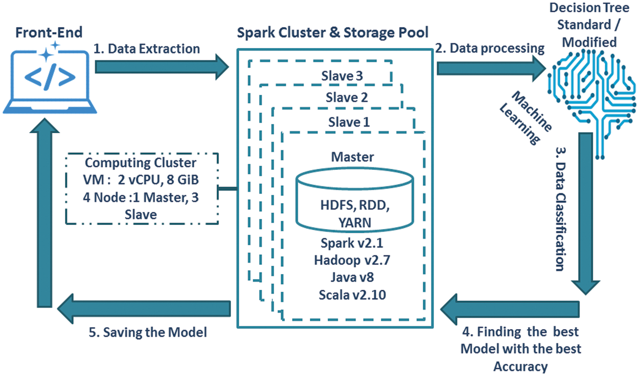
Figure 1: Overview of our proposed methodology

3.1 Input Data

In this study, we used two datasets: airport and fire call service datasets.

3.2 Data Extraction and Processing Phase

This phase consists of data cleansing, integration, and transformation. A major focus here is getting data ready for categorization. Cleaning the data is necessary before classifier algorithms can be applied to it for analysis. The data imputation process includes removing records with missing values and correcting inconsistencies, identifying outliers, and removing duplicate data. In order to be fed into the data mining program, the information was denoted by numbers and saved as a CSV or txt file.

There should be no empty cells, not even a “not a number (NaN),” or any incorrectly rendered strings in the “data store,” that might interrupt the execution of the program and result in incorrect indication. Preprocessing procedures were employed for clean-up. Zero was given to NaN and empty cells. Then, the decoding procedure began, where the letters were recognized. MATLAB is used to determine the unique list, and then a unique digital code is assigned to each item on the list. Decoding the strings requires a digit between 1 and 26 to be assigned to each letter of the alphabet A.

3.3 Apache Spark Standalone Cluster on Amazon Web Services

Amazon web services were used to get all the data. Elastic cloud computing is a web service for launching and managing virtual machine instances in a virtual computing environment. In this case, we use Ubuntu Server 16.04 LTS (HVM), EBS general-purpose volume type. Canonical (http://www.ubuntu.com/cloud/services) offers assistance.

Amazon offers a variety of instance types, each with a particular set of performance specifications. An Amazon EC2 computing unit serves as the basis for vCPU capacity. A 2007 Opteron or 2007 Xeon processor clocked at 1.0–1.2 GHz roughly represents one EC2 computing unit. Build a standalone Spark cluster on top of Hadoop. We suggest using M4 large spot instances with 200 GB of magnetic hard drive space because of Spark’s memory requirements.

M4 instances are the newest generation of general-purpose instances. Many applications may benefit from this family’s mix of computing, memory, and network resources. There are no extra costs for EBS-optimized E5-2686 v4 or E5-2676 v3 processors in M4 features. There is also support for enhanced networking and an even distribution of processing, memory, and network resources. As the name suggests, this instance type contains four computing units and eight gigabytes of memory, making it ideal for large-scale web applications that need enormous amounts of processing power.

One of the nodes will be designated as the master (Name Node), and the other three will be designated as slave (Data Nodes). Gigabit Ethernet connects the nodes. The binaries built on Lawrencium were used on EC2 for consistency. The nodes are in the same availability zone in the N. California area. Moreover, Amazon gives no assurances as to the closeness of the nodes placed together, and the latency between nodes varies widely. Apache Spark v2.1.0, Apache Hadoop v2.6.1, Java v8, and Scala v2.11.0 were used in the experiments.

Furthermore, we used distributed memory for fault-tolerant calculations on a cluster using Spark. Even though Spark is a relatively young open-source technology, it has already overtaken Hadoop’s MapReduce approach in terms of popularity. This is mainly because Spark’s resilient distributed dataset (RDD) [30] architecture can work as MapReduce paradigm. With Spark MLlib, machine learning algorithms can be run significantly quicker than with Hadoop alone because of its ability to execute iterative computations on large datasets.

Our methods are implemented using the Apache Spark cluster computing framework to handle datasets that are too large to be stored and processed on a single node. The fault-tolerant parallel and distributed computing paradigm and execution engine provided by Spark are based on RDD. Functional programming techniques, such as map, filter, and reduce, each yield a new RDD when performed on an RDD. RDDs are immutable, lazily materialized distributed collections. Data may be retrieved from a distributed file system or produced by parallelizing a data collection that the user has already made.

There are many operations that are possible with RDDs containing key-value pairs that may be applied to them as associative arrays. In order to save time, Spark employs a lazy evaluation method. One of the key advantages of Spark over MapReduce is the use of in-memory storage and caching to reuse data structures. Hadoop has three components, and it is vital to have a general understanding before its implementation.

•   Files are divided into “blocks” and stored redundantly on numerous low-cost workstations known as “Data Nodes” using the Hadoop distributed file system (HDFS) [29]. HDFS is based on the Google file system [25–31]. Moreover, the Name Node is a high-quality computer that serves as the point of entry to these data nodes.

•   Hadoop MapReduce (based on Google MapReduce) is a distributed computing paradigm that divides calculations across numerous computers. Each computer in the cluster performs a user-defined function on a slice of the input data in the Map job. In the Reduce task, the output of the Map job is shuffled throughout the cluster of workstations.

•   A new feature in Hadoop 2.0 known as YARN (unofficially known as yet another resource negotiator) handles resources and task scheduling like an operating system. This is an essential enhancement, particularly in production with several programs and users, but we will not focus on this for now.

Finally, the scholars were employed during the experimentation: a master and three workers, each with two virtual central processing units and eight gigabytes of RAM, and four same-level clusters were used to complete the jobs quicker. Amazon platform built the infrastructure. Apache Spark v2.1.0, Apache Hadoop v2.6.1, Java v8, and Scala v2.11.0 were used in the experiments. Apache Spark is a high-performance in-memory computing platform intended to be one of the fastest available and extremely general-purpose in terms of conducting many types of computing tasks.

3.4 Finding the Accurate Model

After the data processing and classification phase, we propose a model using a multi-layer to build an environment by determining the number of nodes. Then, we prepare programming language libraries used in the environment, such as Java v8 and Scala v2.11, and continue downloading all layers. The first layer is an Apache Hadoop v2.7 (MapReduce, HDFS, YARN), and the second layer is an Apache Spark, including the number of cores. All the layers are downloaded on all nodes used in the environment. The accurate choice model is based on several features; one of the most important is accuracy. All of them depend on a dataset. Finally, save and load the accurate model.

3.5 Evaluation Measures

The proposed model is evaluated using different evaluation metrics, including recall, precision, accuracy, and F1-score. These metrics depend on true positive (TP), true negative (TN), false positive (FP), and false negative (FN), which are common evaluation parameters for predictive models.

Accuracy (Acc) is expressed as in Eq. (1):

Acc=TP+TNTP+TN+FP+FN(1)

Precision (P) [20], which equals TP divided by TP+FP, is expressed as in Eq. (2).

P=TPTP+FP(2)

Recall (R) [20], which equals (TP) divided by TP+FN, is expressed as in Eq. (3).

R=TPTP+FN(3)

F-Measure (F1) [20], which is equal to twice the precision multiplied by recall divided by the sum of precision and recall is written as Eq. (4).

F1=2∗Precision∗RecallPrecision+Recall(4)

A receiver operating characteristic (ROC) or ROC curve is a graphical plot that shows the performance of a binary classifier system as the discernment threshold is diverse.

Area under the precision-recall curve (PRC): Tuning the prediction threshold will change the precision and recall of the model, and it is an imperative part of model optimization. It plots (precision, recall) points for diverse threshold values; ROC curve plots (recall, FP rate) points.

Mean squared error (MSE) is a variance of the estimator and what is estimated. It is a risk function, consistent with the estimated value of the squared error or quadratic loss.

Root mean square error (RMSE) is often used to measure the variances between values predicted by a model or an estimator and the values actually detected.

4  Equations and Mathematical Expressions

In this section, we first present the standard DT, followed by the improved DT. Then, we compare the two DT algorithms.

4.1 Standard DT

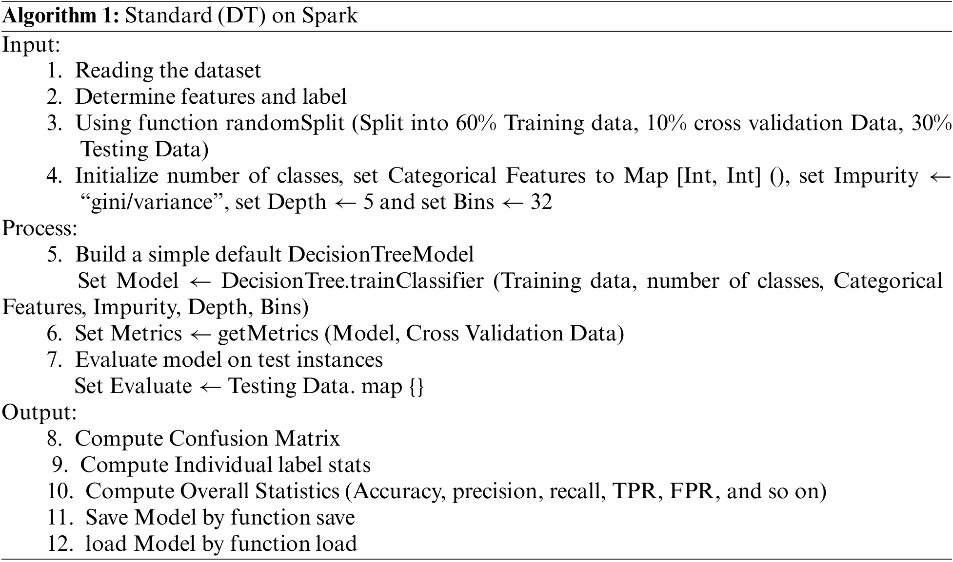
We have all the essential components to demonstrate how Algorithm 1’s (DT) implementation works. It is built on the Spark MLlib source code as a model implementation. To import a data file and parse it into an RDD of a labeled point, see Algorithm 1. The dataset was divided into training, cross-validation, and test sets, consisting of 60%, 10%, and 30% of the dataset, respectively. We used five parameters to build the DT model, including the number of classes, number of bins, categorical characteristics, impurity, and number of depths. The algorithm can produce more precise split judgments when increasing the maximum number of bins. Additionally, it raises computational and communication demands. Consider that the max-bin parameter must be greater than or equal to the maximum number of categorical features. How many values can each feature have? That is the question that categorical features answer. This is presented as a feature index-to-arity mapping (number of categories) using DT with a Gini impurity measure or DT with a variance impurity measure and a tree depth of 5 for classification or regression. Once a test error is generated, MSE is produced to evaluate the algorithm’s correctness.

4.2 Enhancement of DT

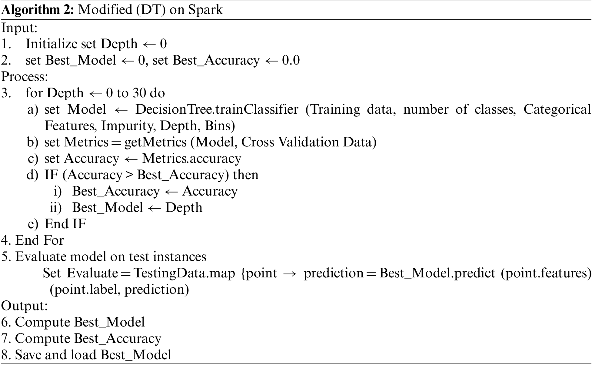
Algorithm 2’s enhancement (DT) implementation may now be explained using the relevant components. The algorithm requires some parameters; however, we make self-tuning running parameters based on the depth. Classification or regression may be performed using DT using Gini or variance impurity as an impurity metric. We iterate with an initial depth of zero, increasing it incrementally to thirty, building the model. Additionally, we compare it with the best accuracy. Finally, we create the best model with the best accuracy.

5  Result and Analysis

This section presents the experimental results of our proposed model. The datasets used to verify the effectiveness of the proposed model are described in Subsection 5.1. We present the working environment in Subsection 5.2. Furthermore, we present the comparative analysis in Subsections 5.3 and 5.4.

5.1 Datasets Description

We use two datasets in our experiment. The first is a huge dataset initially created by the Research & Innovative Technology Administration. Five classes, 29 characteristics, and 86 features are included in the dataset, approximately 500,000 instances. The second large dataset was provided by San Francisco domestic fire department calls for service. The dataset consists of nearly 600,000 instances with five classes and 35 attributes. All datasets should have correct feature extraction and feature selection performed.

5.2 Working Environment

The simulation results have been carried out on the FN data using a local machine with an Intel processor core i7, 16 GB of RAM, and an NVIDIA GTX 1050i GPU.

5.3 Classification Results and Performance Evaluation on First Dataset

There is no difference between the experimental results with a multi-node or local (one node) environment. The only difference is that the time also depends on the number of nodes shown in the next table. Fig. 2 shows the accuracy results for the standard and modified DT algorithms tested on the airport dataset using the Apache Spark mining tool. The x-axis represents the results of the accuracy (correctly classified and incorrectly classified instances), whereas the y-axis represents the modified and standard algorithms. The standard and modified DTs are represented in blue and red, respectively.

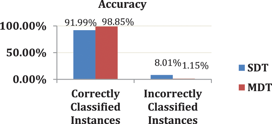
Figure 2: A comparative study of accuracy percentage between modified decision tree (DT) algorithm and standard (DT) using Apache spark with the airport dataset

Table 1 compares the standard DT cluster with the local using the airport dataset. The results in this table present the time needed to build the model in seconds, where the time is calculated using the Apache Spark mining tool. In this study, the results of time vary based on the cluster (multi-node) or local (one node). The time to build the standard DT model with cluster (four nodes) and local (one node) are 426 and 660 s, respectively.

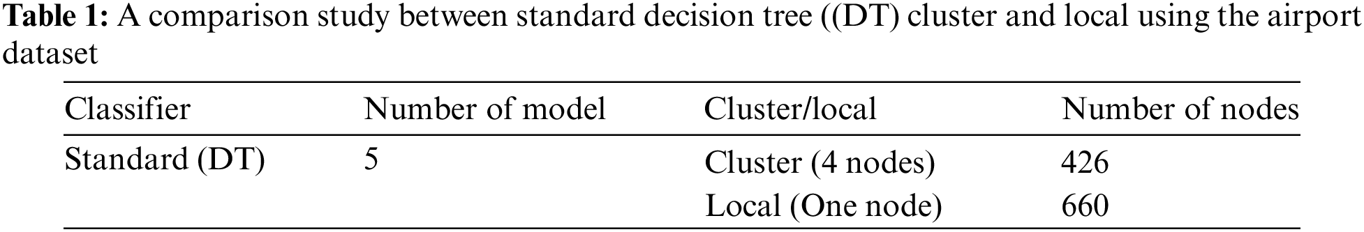
Table 2 compares the results of the modified DT cluster and local using the airport dataset. This table shows the time needed to build the model in seconds, where time is calculated using the Apache Spark mining tool. Here, the results of time vary based on the cluster (multi-node) or local (one node). The time to build the modified DT model in the first and second runs with cluster (four nodes) are 2640 and 482 s, respectively. In contrast, the time to build the modified DT model in the first and second runs with local is 7680 and 666 s, respectively. The variances for the modified DT model with local are three times more than those in the cluster.

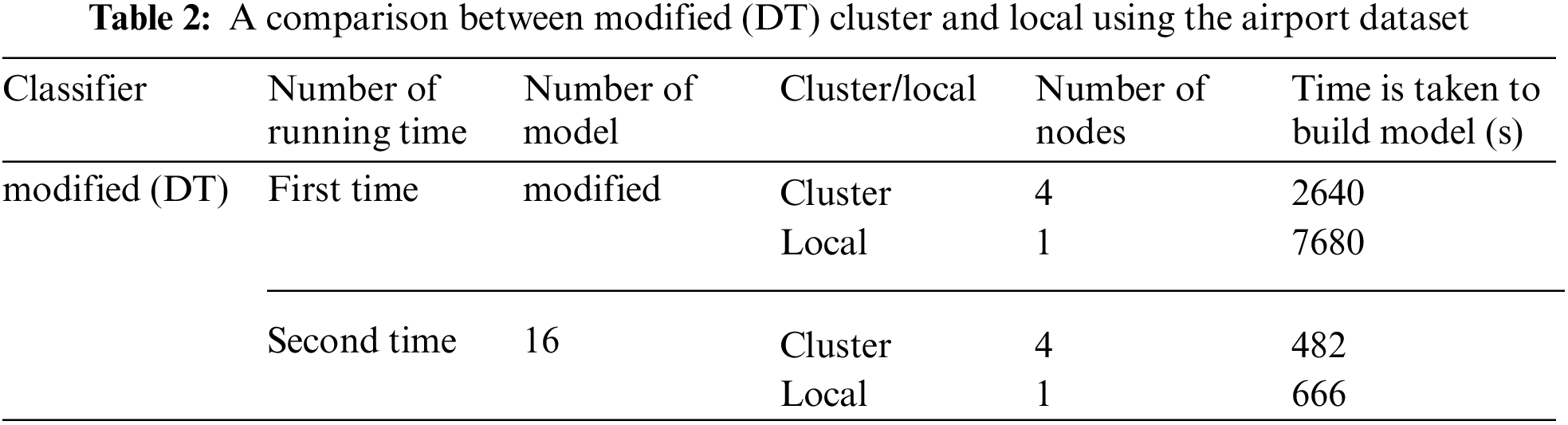
Table 3 compares the results of the standard DT and modified DT algorithms in the cluster using the airport dataset. This table shows the time needed to build the model in seconds, where the time is calculated using the Apache Spark mining tool. The time to build the modified DT model in the first run is 2640 s, whereas the time to build the modified DT when putting the number of models 16 is 482 s with four nodes for both. The study shows that when we put the number of models, it takes five times the first run. The time to build the standard DT model with four nodes is 426 s, whereas the time to build the modified DT when putting the number of models 16 is 482 s.

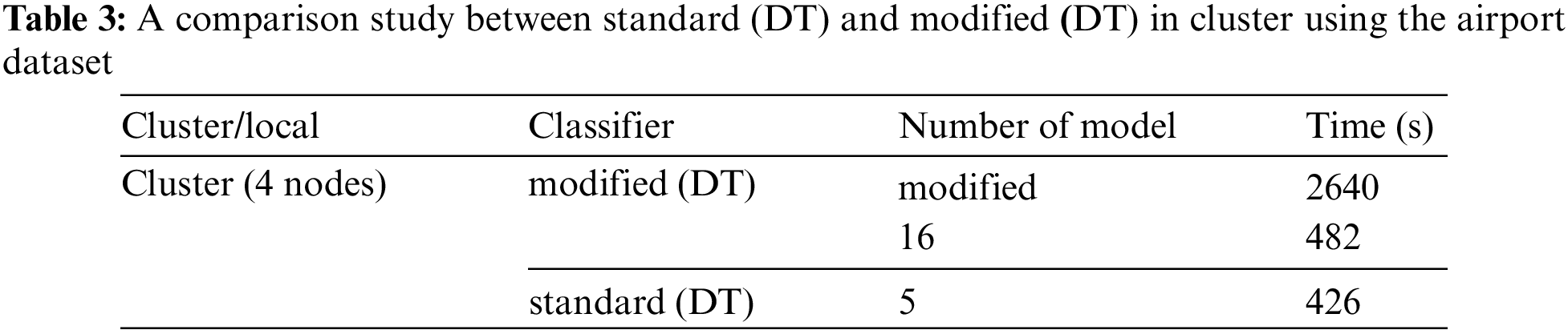
Table 4 compares the results of the standard and modified DT models in local using the airport dataset. This table shows the time needed to build the model in seconds, where the time is calculated using the Apache Spark mining tool. The time to build the modified DT model in the first run is 7680 s, whereas the time to build the modified DT model when putting the number of models as 16 is 666 s with one node for both. The study shows that when we put the number of models, the results of the time change at a percentage equal to eleven times the result for the first time. The time to build the modified DT model with one node is 660 s, whereas that of the modified DT when putting the number of models 16 is 666 s.

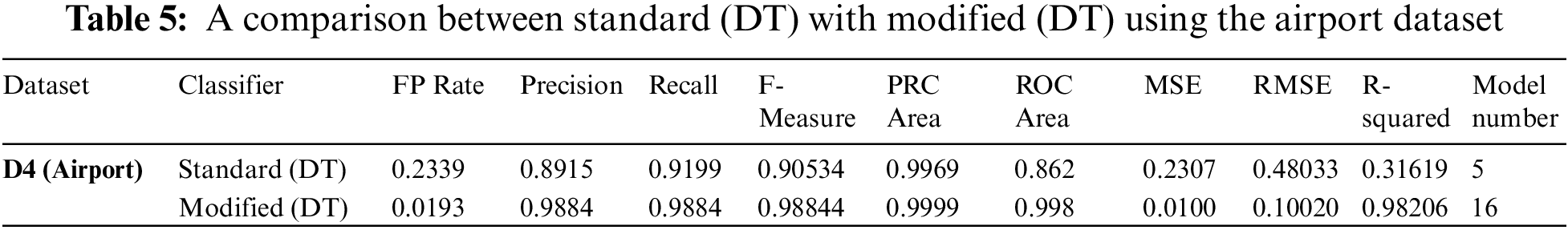
Table 5 shows the FP rate, recall, and precision of the first datasets, along with the number of models. A look at the data reveals that the modified DT has the greatest value for most parameters by 6.85% and the lowest good value of MSE at 0.0100 because a value closer to zero is better. External predictability may be shown by an R-squared prediction value larger than 0.6. The RMSE values of 0.5 and 0.3 should be low for a decent prediction model. Both are a better value and good external of RMSE. The modified DT is better than the standard DT because the value of RMSE at 0.10020 is less than 0.3, and the standard DT is greater than 0.3 but still a good predictive model. The modified DT has a better value and good external R-squared at 0.98206, whereas the standard DT has poor external predictability at 0.31619.

Finally, the comparison study made between the standard and modified DT algorithms aid in attaining high accuracy in various datasets. The top method was the modified DT algorithm, which had a 98.84% accuracy rate with a total construction of 2640 s. As shown, the modified DT has the highest value of all parameters by 6.85%.

5.4 Classification Results and Performance Evaluation on Second Dataset

There is no difference between the experimental results with a multi-node or local (one node) environment. The only difference is that the time also depends on the number of nodes shown in the next table. Fig. 3 shows the accuracy results of the standard and modified DT algorithms tested on the fire call service dataset using the Apache Spark mining tool. The x-axis represents the results of the accuracy (correctly classified and incorrectly classified instances), whereas the y-axis represents the modified and standard DT algorithms. The standard and modified DT models are represented in blue and red, respectively.

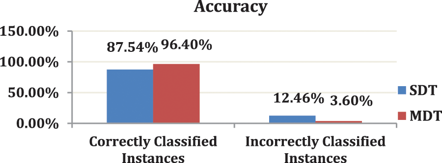
Figure 3: A comparative study of accuracy percentage between modified (DT) algorithm and standard (DT) using Apache spark with fire dataset

Table 6 compares the results of the standard DT in the cluster and local environments using the fire dataset. These results show the time needed to build the model in seconds, where the time is calculated using the Apache Spark mining tool. Here, the time results vary widely based on the cluster (four nodes) or local environment (one node). The time to build the standard DT model with the cluster (four nodes) and local environment are 129 and 367, respectively.

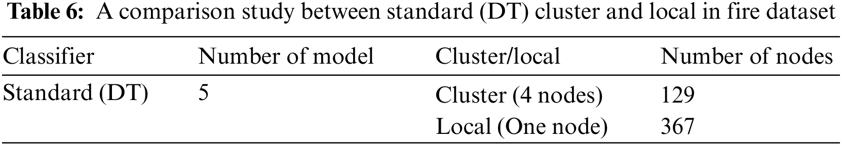
Table 7 compares the results of the modified DT in the cluster and local environments using the fire dataset. These results show the time needed to build the model in seconds, where the time is calculated using the Apache Spark mining tool. Here, the time results vary widely based on the cluster (four nodes) or local environment (one node). The time to build the modified DT model in the first run in the cluster (four nodes) is 2280 s, and that when putting the number of model 12 with the same number of nodes is 187 s. In contrast, the time to build the modified DT model in the first run in the local environment is 3780 s and that when putting the number of model 12 with the same number of nodes (one node) is 365 s. The variances of the DT in the first run in the local environment are more than one and half times that in the cluster environment.

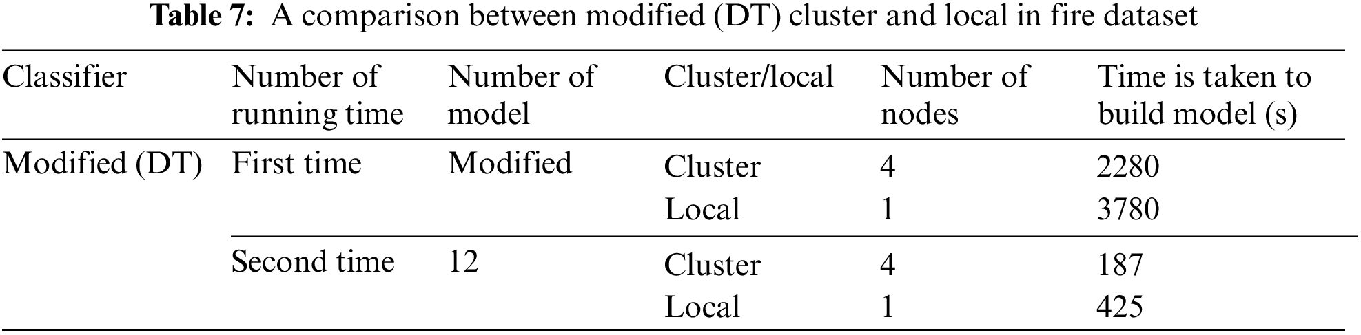
Table 8 compares the results of the standard and modified DT algorithms in the cluster environment using the fire dataset. This table shows the time needed to build the model in seconds, where the time is calculated using the Apache Spark mining tool. The time to build the modified DT model in the first run is 2280 s, whereas that when putting the number of model 12 is 187 s in the cluster (four nodes). Here when putting the number of models, the time results change at a percentage equal to twelve times the result for the first time. The time to build the standard DT model with four nodes is 129 s, whereas that putting the number of models 12 is 187 s.

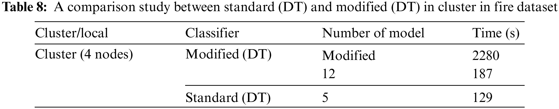
Table 9 compares the results of the standard and modified DT in the local environment using the fire dataset. These results show the time needed to build the model in seconds, where the time is calculated using the Apache Spark mining tool. The time to build the modified DT model in the first run is 3780 s, whereas that when putting the number of models 12 is 425 s with one node for both. When we put the number of models, the time results change at a percentage equal to ten times the result for the first time. The time to build the standard DT model with one node is 367 s, whereas that to build the modified DT when putting the number of models 12 is 425 s.

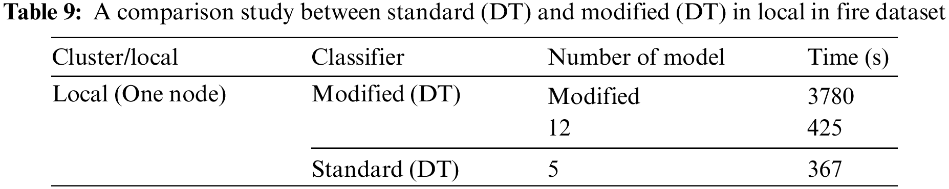
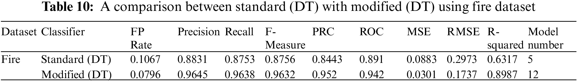
Table 10 shows the first dataset: FP rate, precision, recall, F-measure, PRC area, ROC area, and the number of models. Modified decisions are shown in the table. The modified DT has an 8% higher value for most factors, as shown in the table. Since a value closer to zero is preferable, the modified (DT) has the lowest and best MSE of 0.03019. The RMSE values should be low (0.5 and 0.3) for a decent prediction model. Both have better values and good external RMSE because they have good predictions under the rule <0.3. External predictability may be shown by the R-squared prediction value greater than 0.6. The modified and standard DT models have better values and good external R-squared at 0.8987 and 0.63170, respectively.

Finally, the comparison study between the standard and modified DT algorithms helps attain high accuracy in various datasets. The modified DT method was the most accurate and took the least time to create, with 96.4% accuracy and a total duration of 2280 s. As shown, the modified DT has the highest value of all parameters by 8%.

5.5 Managerial Implications

The proposed modified DT approach aims to achieve optimal depth by self-tuning running parameters and improving the performance. The modified DT can achieve higher accuracy in terms of training, validation, and testing than the standard DT. It plays an essential role as a daily-accessed decision-making system that can support the strategic and practical implications of decision-making in organizations for top management, particularly in developing countries. This study attempts to contribute to the literature with new findings and recommendations. These fallouts will help the top management during the key decision-making process and encourage practitioners who seek a competitive advantage through enhanced organizational performance in small and medium enterprises.

6  Conclusion

Big data analytics has attracted significant attention from business and academia because of its tremendous cost-cutting and decision-making advantages. For example, it can provide important information for a wide range of businesses. Therefore, in this study, we proposed a modified DT approach for handling big data. For normal cases while using (DTs), the model is static. Therefore, this study should be more dynamic than the benchmark by allowing the tree to create a new model that fits the dataset. One drawback of making the structure of the model dynamic when determining which model will fit is that it takes more time than the standard model at once, but there are more accurate parameters because the model will certainly fit. However, after using the same model of the modified DT in the second time, it takes approximately the same time as the standard model. Additionally, the number of nodes is taken as a measurement factor to evaluate the time. The time results taken to build the model with multiple nodes (four nodes) within the cluster are less than that with local (one node). Finally, the modified DT achieves an optimal depth by self-tuning running parameters and improving the performance. The efficiency and efficacy of the modified DT were verified using two datasets: airport and fire. The airport and fire datasets contain 500000 and 600000 instances, respectively. Furthermore, we compared the modified and standard DT, and the comparison results showed that the modified DT performs better than the standard DT. This comparison was conducted on multi-node using the Apache Spark tool with Amazon web services, resulting in an increase in the accuracy of 6.85% and 8.85% for the fire and airport datasets, respectively. The main limitations of this study are that the proposed modified DT takes longer than the standard DT. Although the proposed model achieved an accuracy higher than standard (DT), it still needs more modifications to achieve better results. In future studies, we will improve the proposed model to achieve the highest accuracy and minimize the execution time. This will be implemented on a cluster and big data from various sources.

Funding Statement: The authors received no specific funding for this study.

Conflicts of Interest: The authors declare that they have no conflicts of interest to report regarding the present study.

Supplementary Materials: The authors received no supplemental materials for this study.

References

    1. D. Ramos, P. Faria, A. Morais and Z. Vale, “Using decision tree to select forecasting algorithms in distinct electricity consumption context of an office building,” Energy Reports, vol. 8, no. 3, pp. 417–422, 2022. [Google Scholar]

    2. M. Li, P. Vanberkel and X. Zhong, “Predicting ambulance offload delay using a hybrid decision tree model,” Socio-Economic Planning Sciences, vol. 80, no. 1, pp. 101146, 2022. [Google Scholar]

    3. M. M. Hafez, R. P. D. Redondo and A. F. Vilas, “A comparative performance study of Naïve and ensemble algorithms for E-commerce,” in 14th Int. Computer Engineering Conf. (ICENCO), Cairo, Egypt, pp. 26–31, 2019. [Google Scholar]

    4. A. M. Shah, X. Yan, S. A. A. Shah and G. Mamirkulova, “Mining patient opinion to evaluate the service quality in healthcare: A deep-learning approach,” Journal of Ambient Intelligence and Humanized Computing, vol. 11, no. 5, pp. 2925–2942, 2020. [Google Scholar]

    5. A. M. Shah, X. Yan, S. Tariq and M. Ali, “What patients like or dislike in physicians: Analyzing drivers of patient satisfaction and dissatisfaction using a digital topic modeling approach,” Information Processing & Management, vol. 58, no. 3, pp. 102516, 2021. [Google Scholar]

    6. C. Magazzino, M. Mele, N. Schneider and U. Shahzad, “Does export product diversification spur energy demand in the APEC region? Application of a new neural networks experiment and a decision tree model,” Energy and Buildings, vol. 258, no. 1, pp. 111820, 2022. [Google Scholar]

    7. K. Saleh and A. Ayad, “Fault zone identification and phase selection for microgrids using decision trees ensemble,” International Journal of Electrical Power & Energy Systems, vol. 132, no. 1, pp. 107178, 2021. [Google Scholar]

    8. Y. An and H. Zhou, “Short term effect evaluation model of rural energy construction revitalization based on ID3 decision tree algorithm,” Energy Reports, vol. 8, no. 1, pp. 1004–1012, 2022. [Google Scholar]

    9. F. M. Javed Mehedi Shamrat, R. Ranjan, K. M. Hasib, A. Yadav and A. H. Siddique, “Performance evaluation among ID3, C4.5, and CART decision tree algorithm,” Pervasive Computing and Social Networking, vol. 317, no. 1, pp. 127–142, 2022. [Google Scholar]

  10. F. Tempola, M. Muhammad, A. K. Maswara and R. Rosihan, “Rule formation application based on C4. 5 algorithm for household electricity usage prediction,” Trends in Sciences, vol. 19, no. 3, pp. 2167–2167, 2022. [Google Scholar]

  11. C. Stachniss, G. Grisetti and W. Burgard, “Information gain-based exploration using rao-blackwellized particle filters,” Robotics: Science and Systems, vol. 2, no. 1, pp. 65–72, 2005. [Google Scholar]

  12. J. L. Grabmeier and L. A. Lambe, “Decision trees for binary classification variables grow equally with the Gini impurity measure and Pearson’s chi-square test,” International Journal of Business Intelligence and Data Mining, vol. 2, no. 2, pp. 213–226, 2007. [Google Scholar]

  13. B. Charbuty and A. Abdulazeez, “Classification based on decision tree algorithm for machine learning,” Journal of Applied Science and Technology Trends, vol. 2, no. 1, pp. 20–28, 2021. [Google Scholar]

  14. F. Rahimibashar, A. C. Miller, M. Salesi, M. Bagheri, A. Vahedian-Azimi et al., “Risk factors, time to onset and recurrence of delirium in a mixed medical-surgical ICU population: A secondary analysis using Cox and CHAID decision tree modeling,” EXCLI Journal, vol. 21, no. 1, pp. 30–30, 2022. [Google Scholar]

  15. N. A. K. Dam, T. Le Dinh and W. Menvielle, “The quest for customer intelligence to support marketing decisions: A knowledge-based framework,” Vietnam Journal of Computer Science, vol. 9, no. 1, pp. 1–20, 2022. [Google Scholar]

  16. S. Kaul, S. A. Fayaz, M. Zaman and M. A. Butt, “Is decision tree obsolete in its original form? A burning debate,” Revue D’Intelligence Artificielle, vol. 36, no. 1, pp. 105–113, 2022. [Google Scholar]

  17. W. Fan, B. Xu, H. Li, G. Lu and Z. Liu, “A novel surrogate model for channel geometry optimization of PEM fuel cell based on bagging-SVM ensemble regression,” Int. J. Hydrogen Energy, vol. 47, no. 33, pp. 14971–14982, 2022. [Google Scholar]

  18. A. Almas, M. Farquad, N. R. Avala and J. Sultana, “Enhancing the performance of decision tree: A research study of dealing with unbalanced data,” in Seventh Int. Conf. on Digital Information Management (ICDIM), Macao, China, pp. 7–10, 2012. [Google Scholar]

  19. H. Kaur and A. Sharma, “Improved email spam classification method using integrated particle swarm optimization and decision tree,” in 2nd Int. Conf. on Next Generation Computing Technologies (NGCT), Dehradun, India, pp. 516–521, 2016. [Google Scholar]

  20. S. Sriram and X. Yuan, “An enhanced approach for classifying emotions using customized decision tree algorithm,” in 2012 Proc. of IEEE Southeastcon, Orlando, FL, USA, pp. 1–6, 2012. [Google Scholar]

  21. M. Ijaz, M. Attique and Y. Son, “Data-driven cervical cancer prediction model with outlier detection and over-sampling methods,” Sensors, vol. 20, no. 10, pp. 2809, 2020. [Google Scholar]

  22. J. Tamang, J. Nkapkop, M. Ijaz, P. Prasad and N. Tsafack, “Dynamical properties of ion-acoustic waves in space plasma and its application to image encryption,” IEEE Access, vol. 9, no. 1, pp. 18762–18782, 2021. [Google Scholar]

  23. G. Alfian, M. Syafrudin, M. F. Ijaz, M. A. Syaekhoni and N. L. Fitriyani, “A personalized healthcare monitoring system for diabetic patients by utilizing BLE-based sensors and real-time data processing,” Sensors, vol. 18, no. 7, pp. 2183, 2018. [Google Scholar]

  24. M. F. Ijaz, G. Alfian, M. Syafrudin and J. Rhee, “Hybrid prediction model for type 2 diabetes and hypertension using DBSCAN-based outlier detection, synthetic minority over sampling technique (SMOTEand random forest,” Applied Sciences, vol. 8, no. 8, pp. 1325, 2018. [Google Scholar]

  25. M. M. Hafez, M. E. Shehab, E. El Fakharany and A. E. F. A. G. Hegazy, “Effective selection of machine learning algorithms for big data analytics using apache spark,” International Conference on Advanced Intelligent Systems and Informatics, vol. 533, pp. 692–704, 2016. [Google Scholar]

  26. A. Esmaeilzadeh, M. Heidari, R. Abdolazimi, P. Hajibabaee and M. Malekzadeh, “Efficient large scale nlp feature engineering with apache spark,” in 12th Annual Computing and Communication Workshop and Conf. (CCWC), Las Vegas, USA, pp. 0274–0280, 2022. [Google Scholar]

  27. B. T. Hasan and D. B. Abdullah, “A survey of scheduling tasks in big data: Apache spark,” Micro-Electronics and Telecommunication Engineering, vol. 373, pp. 405–414, 2022. [Google Scholar]

  28. N. Fikri, M. Rida, N. Abghour, K. Moussaid and A. Elomri, “WS-PDC: Persistent distributed channel-based web services applied on IFRS data processing and loading,” Proceedings of Sixth International Congress on Information and Communication Technology, vol. 235, pp. 847–855, 2022. [Google Scholar]

  29. P. MacKo and J. Hennessey, “Survey of distributed file system design choices,” ACM Transactions on Storage, vol. 18, no. 1, pp. 1–34, 2022. [Google Scholar]

  30. S. Ghemawat, H. Gobioff, and S. -T. Leung Google, “The google file system,” in Proc. of the Nineteenth ACM Symp. on Operating Systems Principles, New York, USA, pp. 29–43, 2003. [Google Scholar]

  31. R. Vijayakumari, R. Kirankumar, and K. G. Rao, “Comparative analysis of google file system and hadoop distributed file system,” International Journal of Advanced Trends in Computer Science and Engineering, vol. 3, pp. 553–558, 2014. [Google Scholar]