
 Submit a Paper
 Propose a Special lssue
 Open Access
ARTICLE

Adaptive Noise Detector and Partition Filter for Image Restoration
1 School of Information and Communication Engineering, Hainan University, Haikou, 570228, China
2 State Key Laboratory of Marine Resource Utilization in South China Sea, HainanUniversity, Haikou, 570228, China
* Corresponding Authors: Siling Feng. Email: ; Mengxing Huang. Email:
Computers, Materials & Continua 2023, 75(2), 4317-4340. https://doi.org/10.32604/cmc.2023.036249
Received 22 September 2022; Accepted 08 February 2023; Issue published 31 March 2023
 View Full Text
 Download PDF
Abstract
The random-value impulse noise (RVIN) detection approach in image denoising, which is dependent on manually defined detection thresholds or local window information, does not have strong generalization performance and cannot successfully cope with damaged pictures with high noise levels. The fusion of the K-means clustering approach in the noise detection stage is reviewed in this research, and the internal relationship between the flat region and the detail area of the damaged picture is thoroughly explored to suggest an unique two-stage method for gray image denoising. Based on the concept of pixel clustering and grouping, all pixels in the damaged picture are separated into various groups based on gray distance similarity features, and the best detection threshold of each group is solved to identify the noise. In the noise reduction step, a partition decision filter based on the gray value characteristics of pixels in the flat and detail areas is given. For the noise pixels in flat and detail areas, local consensus index (LCI) weighted filter and edge direction filter are designed respectively to recover the pixels damaged by the RVIN. The experimental results show that the accuracy of the proposed noise detection method is more than 90%, and is superior to most mainstream methods. At the same time, the proposed filtering method not only has good noise reduction and generalization performance for natural images and medical images with medium and high noise but also is superior to other advanced filtering technologies in visual effect and objective quality evaluation.Keywords
Image restoration and transformation is a subfield of computer vision that includes techniques like denoising, watermark removal, and hyper-segmentation. Advanced image processing tasks like contour extraction, object identification, and text extraction are greatly hindered by the presence of noise and watermarks in the original picture. Picture watermarking, from a pixel-level perspective, alters the gray value of pixels in certain regions of an image. For this reason, watermarking may also be thought of as noise. Therefore, it is helpful to propose new strategies for picture watermarking by enhancing a good denoising model [1].
The image-denoising model can be expressed as Y = X + B, where Y and X represent damaged image and clear image respectively, and B denotes the adaptive noise. The noises in natural images and medical images are mainly Gaussian noise, Poisson noise, multiplicative noise and random-value impulse noise (RVIN). Fig. 1 shows the damage to four kinds of noises to the picture, where g (x, y) and f (x, y) represent noisy images and clear images respectively, h (x, y), p (*), m (x, y) and η (x, y) respectively represent the distribution functions of different noises. There are many algorithms [2–4] for Gaussian noise removal and the performance is good. Compared with Gaussian noise and other types of noise, the random characteristic of RVIN brings more trouble to noise removal. RVIN is an additive noise, and the gray value of the polluted pixel is independently taken in [0, 255]. The luminance value of RVIN noise pixels can be any value within the allowable range of the luminance value of image pixels. The difference between this value and the luminance value of pixels in the field is usually small, which is difficult to distinguish. Therefore, the removal of RVIN noise is more challenging.
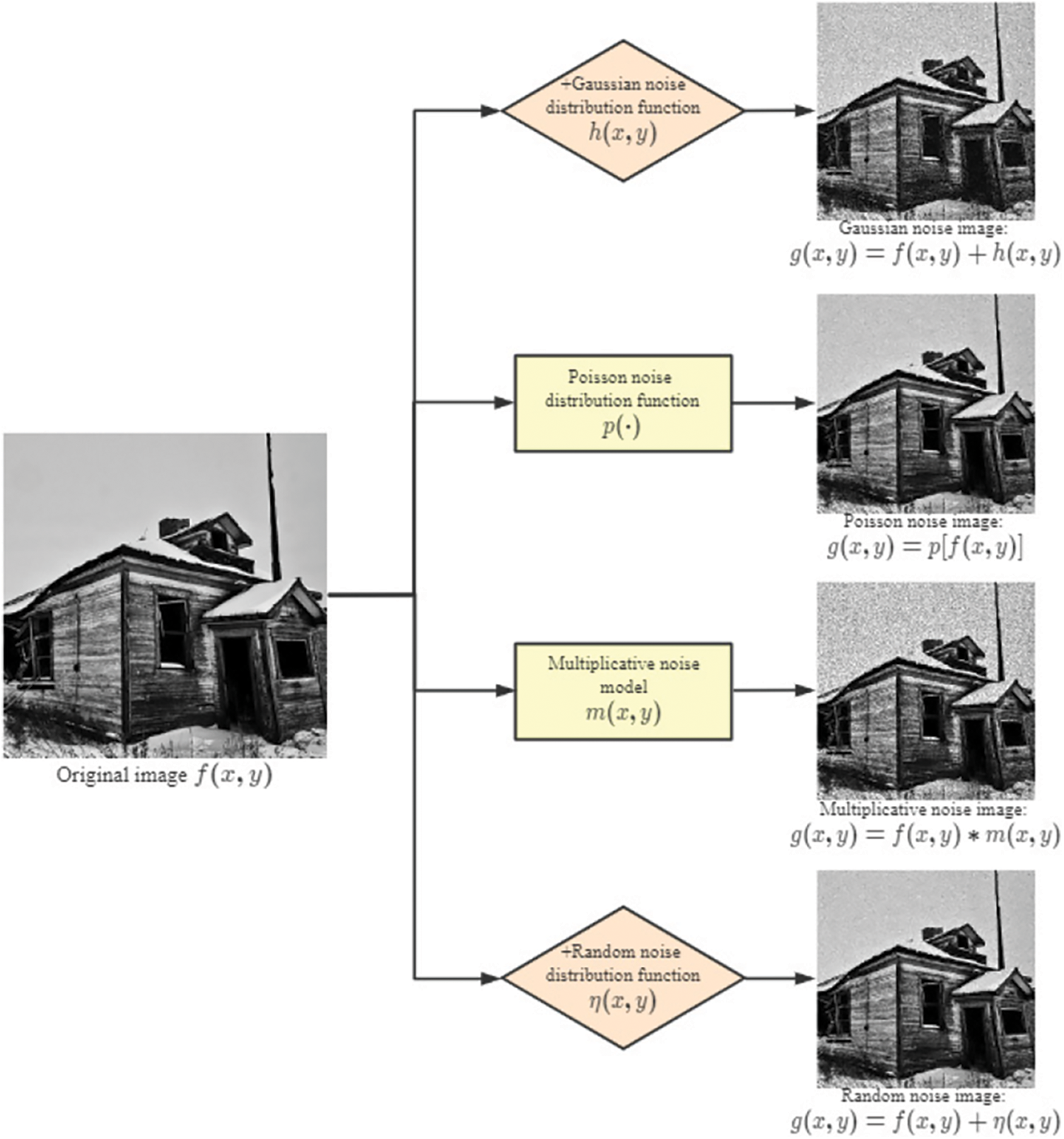
Figure 1: The flowchart of types of noise
Several filters for Gaussian noise removal, such as the Gaussian filter, mean filter and bilateral filter, are tried to remove RVIN. These linear and nonlinear methods combine the spatial information and gray similarity of the image to achieve the purpose of edge-preserving denoising, but the effect on random impulse noise is general. The median filter [5] and its variant weighted median filter (CWM) [6] sort the pixels in the local area according to the gray level, and take the median or weighted median of the gray level in the field as the gray value of the current central pixel. In contrast, they have a good effect on removing impulse noise and solving the problem of blurred details caused by the linear filter in image restoration to a certain extent. Reference [7] proposes a new adaptive weighted median filter (ACWM), which uses the learning method based on the least mean square (LMS) algorithm to obtain the center weight in each block, and then gradually applies it for the noise filtering program through multiple iterations to obtain the optimal filtering effect. However, for images with many detail textures such as points, lines, and spires, these median filters and their improved algorithms are easy to remove the clean pixels in the detail and texture as noise pixels, which cannot fundamentally solve the problems of image blur and loss of detail information.
The two-stage denoising algorithm based on noise detection and filtering can effectively solve the problems of image blur and detail loss by first detecting the noise pixels in the damaged image and then removing them. The denoising effect of this two-stage method is closely related to the accuracy of noise detection [8]. To accurately screen out random impulse noise in damaged images, a noise detection method based on the local rank-ordered absolute difference (ROAD) is proposed in the literature [9], it determines whether the pixel is noise by counting the gray difference between the central pixel in the local window and its adjacent pixels. Inspired by ROAD, Dong et al. [10] enlarges the difference between the central pixel and the pixels in its neighborhood by using the rank-ordered logarithmic difference (ROLD) of the central pixel in the form of a roll, to improve the accuracy of impulse noise detection. Chen et al. [11] proposed a noise detection method based on rank-ordered relative differences (RORD) combined with ROAD and ROLD, but all of them did not consider the statistical information of pixels in the window and the prior knowledge of noise, such as variance and noise level.
Practically, the noise level has a great influence on the selection of noise detection threshold [12]. To make full use of the prior knowledge of image noise level, Literature [13] introduces a noise detection method based on the local consumer's index (LCI). It measures the similarity between the central pixel and other pixels in the neighborhood by calculating the LCI value of the central pixel and then estimates the noise level of the damaged image to set an appropriate LCI threshold to filter out clean pixels and noisy pixels. To improve the accuracy of noise detection, the author obtains the calculation formula of LCI threshold and image noise level through numerous experiments and polynomial fitting. However, for some images with complex texture and serious damage, the LCI value of pixels is generally low, which is easy to increase the number of misjudged pixels when using a single threshold to detect. Reference [14] designed a three-threshold detection method of standard deviation, average value, and the quartile to solve the problem of image denoising under high noise levels. However, this multi-threshold detection method not only increases the complexity of the algorithm but also has little effect on noise detection. It cannot well distinguish the normal pixels and noise pixels in the detail or texture area. To solve this problem, Nadeem et al. [15] designed a fuzzy noise detector based on switching technology, which can distinguish the noise pixels and edge pixels in the detail and texture areas well. In the noise detection stage, a pixel in the image can be recognized as a clean pixel, a noise pixel, or a candidate noise pixel by using an appropriate threshold, but the paper did not specify how to filter the edge pixels from the candidate noise. Literature [16] introduces in detail a method of order road difference (ROD-ROAD) and local image statistical minimum edge pixel difference (MEPD) to identify edge pixels from candidate noise, to prevent edge pixels from being wrongly identified as noise. However, the above detection and filtering methods based on neighborhood pixels only consider the pixel gray value information in a limited window range and do not consider the pixel distribution characteristics of the whole image, which results in the poor generalization performance of the algorithm. Moreover, when the degree of image damage reaches 60% or even higher, these methods are easy to misjudge normal pixels as noise since the reason that the number of noise pixels is more than clean pixels in the detection window.
From the above analysis, it can be seen that the noise detection method based on manually set detection threshold or local window information does not have good generalization performance, nor can it effectively deal with damaged images with a high noise level. To solve these problems, this paper proposes an RVIN detection and removal method based on the idea of grouping clustering, which can achieve fast noise reduction and retain enough detailed information at the same time. The noise detector divides all pixels in the damaged image into several groups according to the characteristics of the pixels, and then recognizes the noise of each group of pixels through the adaptive threshold. The noise detector divides all the pixels in the damaged image into several groups according to the characteristics of the pixels, and then iteratively optimizes the noise detection model and solves the optimal detection threshold for each group to identify the noise. According to the noise detection results, this paper designed a partition decision filter, which uses different filters for noise pixels in different regions to recover pixels damaged by random-valued impulse noise. Extensive experimental results show that the proposed method is suitable for both natural images and medical images with medium and high noise levels. In addition, it is substantially better than other advanced RVIN filtering techniques in terms of visual and objective quality evaluation.
The main contributions in this article are summarized as follows:
(1) Different from the existing image block denoising method, a pixel clustering method is proposed by using the overall and partial information of the damaged image to divide all the pixels of the damaged image into several classes.
(2) The method of [13] is used to calculate the LCI value of pixels, but for pixels at the junction between classes, only the pixels belonging to the same class in their local window are considered when calculating their LCI value. Then, by optimizing the noise detection model, the optimal detection threshold of each group of pixels is obtained to filter out the noise.
(3) A filtering idea of partition decision-making is proposed. The LCI weighted mean filter and edge direction filter are designed to filter the noise pixels in the flat area and detail area, respectively.
(4) The proposed denoising algorithm has high robustness and generalization and has achieved remarkable results in RVIN removal of natural images and medical images, especially at high noise levels.
In this section, several classical two-stage denoising algorithms related to this work are presented. We first briefly review some noise detection schemes based on local window statistics and then introduce improved algorithms based on median or mean filtering.
In the method based on local information statistics, a specific statistic is usually defined, then the statistic of a given pixel is calculated and directly compared with a threshold to detect RVIN [8,17,18]. The rank-ordered absolute difference (ROAD) proposed in the literature [9] is a typical representative of this detection scheme. In ROAD, the absolute difference between the central pixel and other pixels in the neighborhood is first calculated, then sorted in ascending order, and finally, a predefined ROAD detection threshold is used to discriminate whether the central pixel is a clean pixel or a noisy pixel. The ROAD algorithm is suitable for images with low noise levels. To separate the difference between noisy pixels and clean pixels, [10] takes the logarithmic function of the absolute differences to introduce a new statistic ROLD. Compared with ROAD, the detection stage of ROLD has better detection performance because it can more easily distinguish between noisy and non-noisy pixels, and it still works even when the noise density reaches 60%. Since then, researchers have proposed many improved algorithms based on ROAD and ROLD, such as ROR [19] and ROD-ROAD [16].
Inspired by ROAD and bilateral filter [20], Xiao et al. [13] designed a noise detection method based on the local statistic Local Consensus Index. This method determines whether pixel x is noise by calculating the similarity between any pixel x and other pixels in its neighborhood. The specific calculation method is shown in Formulas (1)–(4):
In Formula (1), θ(x, y) indicates the similarity between pixel x and pixel y in the local area. Ωx0 means the 5 × 5 neighborhood of the central pixel x (excluding x), y denotes any pixel in the neighborhood Ωx0, ux and uy represent the grayscale values of pixels x and y, (m, n) and (s, t) are the coordinates of the pixel x and y, respectively. Both σλ and σs are Gaussian kernels, which are used to adjust the influence of spatial distance and gray difference of pixels on θ(x, y). It can be found from Formula (2) that when x is a normal pixel, the value of ζx will be larger due to its high similarity with every other normal pixel in the neighborhood, and vice versa. Therefore, by observing the ζx value of the center pixel x in Formula (3), the possibility of it being a normal pixel can be evaluated. To make the statistic ζx more stable and discriminative, the author performs a normalization operation to restrain it into domain [0, 1] through Formulas (3) and (4), and finally obtains the LCI value of pixel x.
LCI characterizes the probability of whether a pixel is a noise, and the larger the LCI value of a pixel, the more likely it is a normal pixel. By setting an appropriate threshold, clean pixels and noisy pixels of the entire damaged image can be filtered out. To obtain the best detection effect, the author first uses LCI to determine whether the pixel is in a flat area or a detailed area and then uses different LCI thresholds to filter out noise. The method is computationally simple and can quickly detect the RVIN of damaged images without iteration.
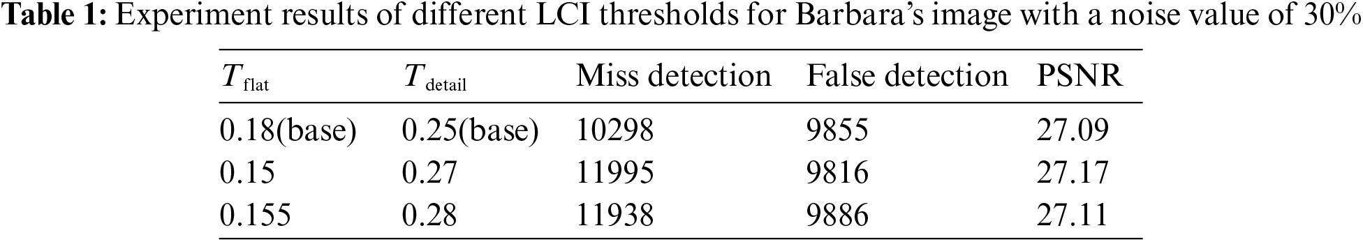
It should be pointed out that the calculation formula of LCI threshold in detail area and flat area are obtained by polynomial fitting after experiments on a large number of test images, which leads to the algorithm not having good robustness. For the LCI detector, the key to judging whether a pixel is a noise pixel is the value of the LCI detection threshold. The more accurately the threshold is set, the more noise pixels are detected. The threshold obtained in [13] needs to be determined by calculating the noise level. Most of the time, the calculated noise level is often deviated from the real pixel level and will increase the amount of calculation. Furthermore, there is a large difference in the composition between images, using a single threshold as the detection standard will lead to large errors in results and poor generalization ability when encountering images with complex texture composition. Table 1 shows the experimental results of different LCI thresholds for Barbara images with a noise value of 30%, when the noise level is 30%, the LCI detection thresholds of the flat area Tflat and the detail area Tdetail can be calculated by the formula given in the literature to be 0.18 and 0.25, respectively, and the noise detection effect and restoration effect of the image are improved to varying degrees when the threshold is changed.
After detecting the RVIN of the image, a filter needs to be designed to remove it. Mean filters use the mean of all pixels in the local window to replace the central pixel. They have been widely used and improved due to their simplicity and speed, but they cannot preserve the edges of the image well. The median filter replaces the noisy pixels with the median value of the filter window while keeping the noise-free pixels unchanged, to better preserve the details and edges of the image [10] proposed a new impulse detector that is aligned with four principal directions based on the difference between the current pixel and its neighbors. Then, it is combined with a weighted median filter (ACWM) to obtain a new directionally weighted median filter (DWM). The median intensity in the filtering window is likely to be a random impulse value as well when the noise density reaches 60% or higher, so this median operation not only fails to remove noise effectively but also introduces other types of impulse noise. Kang et al. [21] proposed a fuzzy inference-based Orientation Median (FRDM) filter, which overcomes the problem of DWM filters. In [22], an adaptive method for threshold selection using fuzzy rules is proposed, which effectively utilizes background pixel information to detect and process noisy pixels.
The median filter and its improvement methods mentioned above can suppress most of the RVIN. However, the filter window has more noisy pixels than clean pixels when the noise level of the damaged image is high, and these methods are still prone to introducing other Noise pixels since the reason that all pixels in the window are involved in filtering during filtering. In addition, the use of a median filter in the flat area of the image is easy to bring obvious burrs to the image. References [7,15] assign weights to the noise or suspected noise in the window to suppress its impact on the central pixel. However, for the pixels damaged by RVIN, the new gray value is a random value, which has no reference significance. Using them to repair the central pixel increases uncertain factors and unnecessary calculation costs. In addition, the existing RVIN denoising algorithms use the same method to deal with any noise in the image, which is unreasonable because the pixel distribution of the flat area and the detail area in the image is very different. The pixel intensity distribution in the flat area A of the image is uniform, and for the uncontaminated noise pixels, the pixel gray value in the local window differs very little. For the detail area, even for the normal pixels in the same local window, the gray difference between them is also great since the reason that the pixel brightness of the image edge and the detail area changes significantly. The gray profile of this area can generally be regarded as a step, that is, one pixel changes sharply in a small buffer area to another pixel with large gray difference. These all show that designing better filters is critical.
3 The Proposed Noise Detection Method
Based on the Section 2.1 analysis, it is believed that setting the LCI detection thresholds of different images or different regions according to the structural characteristics and edge complexity of the image can effectively improve the detection effect of noisy pixels. Noisy pixels are not only characterized by normally distributed random values, but also by random locations in the image. Recently proposed noise detection algorithms are only based on the properties of random values. To take advantage of the second important property of random position, [23] uses a random process model to cluster point patterns formed by random noise, and then according to the relative positions of image pixels, the image pixels of a certain intensity is classified as damaged or undamaged. However, this pixel classification method based on a random process model is too complex and the effect is general. Meanwhile, we noticed that the literature [24] mentioned that pixels in the area surrounded by edge contours in the image have continuity and similarity, and the distance between pixels belonging to the same area will be low. Because of this, the authors use the contour cues of edge-aware geodesic distance to design a structured edge detector to classify the edge regions of the image to deal with the two common problems of occlusion and motion boundaries in optical flow computation. Geodesic distance is also a natural tool for edge-preserving image editing operations (denoising, texture flattening, etc.) [25]. Inspired by references [23] and [24], we think of using the similarity of the geodesic distance between pixels to divide all pixels in the damaged image into several categories, and then when calculating the LCI value of the central pixel, this paper only considers the pixels belonging to the same category in its neighborhood to increase the edge a priori knowledge. Finally, different LCI detection thresholds are set according to the characteristics of each kind of pixel to increase the robustness of the algorithm.
3.1 Clustering and Partition of Image Pixels
Data clustering methods include mean shift clustering, density-based clustering (DBSCAN), Gaussian mixture model (GMM) expectation maximum (EM) clustering, etc. In this paper, the K-means algorithm was used because of its simplicity and fast convergence speed. K-means image clustering segmentation, also known as K-means clustering, uses the principle of unsupervised learning to cluster pixels into several clusters. The specific principles are as follows:
Theorem 1: Given a set of data x1, x2, ..., xn in d-dimensional Euclidean space, assuming that the number of clusters K is known, the points close to each other are clustered into a cluster from the perspective of Euclidean space. The distances between points of different clusters are relatively large.
According to Theorem 3.1, it is necessary to find K clustering centers µk (k = 1, 2,..., K) and assign all pixels in the damaged image to the nearest clustering center, to minimize the square sum of the one-dimensional distance between each pixel and its corresponding clustering center, where the one-dimensional distance refers to the gray difference between them. A binary variable rnk is introduced to represent the attribution of a pixel xn in the damaged image to cluster k, where n = 1, ..., N and k = 1,..., K. If the pixel belongs to the kth cluster, then rnk = 1, otherwise 0. Thus, the following loss function can be defined:
It can be seen from Formula (5) that the initial value of µk needs to be fixed randomly to obtain the attribution value rnk of the pixel that minimizes the loss function J. Given the gray value of pixel xn and cluster center µk, the loss function J is a linear function of rnk. Since xn and xn−1 are independent of each other, for each pixel xn, it is only necessary to assign the point to the nearest cluster center, i.e.,:
Use the rnk obtained in Formula (6) and bring it into Formula (5) to find the cluster center µk. Given the value of rnk, the loss function J is a quadratic function of µk, and makes the derivative of J to µk be 0, then
By Formula (7), it can be deduced that the value of µk is
After the above steps, the pixels of the damaged image will be clustered according to the similarity. Here, the similarity of the pixels is calculated according to the one-dimensional distance between the surrounding pixels and the central cluster pixels. Pixels with the smallest distance from the central cluster are classified into one category. According to the value of K, the pixels of an image can be clustered into K categories. Through pixel clustering, complex image textures can be accurately separated logically, so that class-to-class processing can be realized, and the ability to repair damaged images can be improved to a certain extent. Fig. 2a shows the clustering effect of Lena's image with 50% RVIN when K equals to 4. It can be seen from Fig. 2a that the pixels of the image are divided into four categories, and each category is displayed in different colors. At the same time, for the pixels between classes, because the pixels with certain similarities have been classified in the clustering, the method only needs to take the pixels of the same class in their neighborhood to calculate the LCI when calculating their LCI. As shown in Fig. 2b, for the central pixel of region A, only 8 pixels (221, 32, 64, 22, 112, 23, 23, 74) of the 24 pixels in its neighborhood belong to the same class, then only these few pixels are considered when calculating the LCI value of the center pixel x, thereby increasing the prior knowledge of the edge. It should be pointed out that due to the poor anti-interference of the K-means algorithm, the method will preprocess the simple filtering methods such as median filter or Gaussian filter before clustering and segmentation of images to reduce the impact of noise on clustering effect, so as to meet the requirements of subsequent experiments.
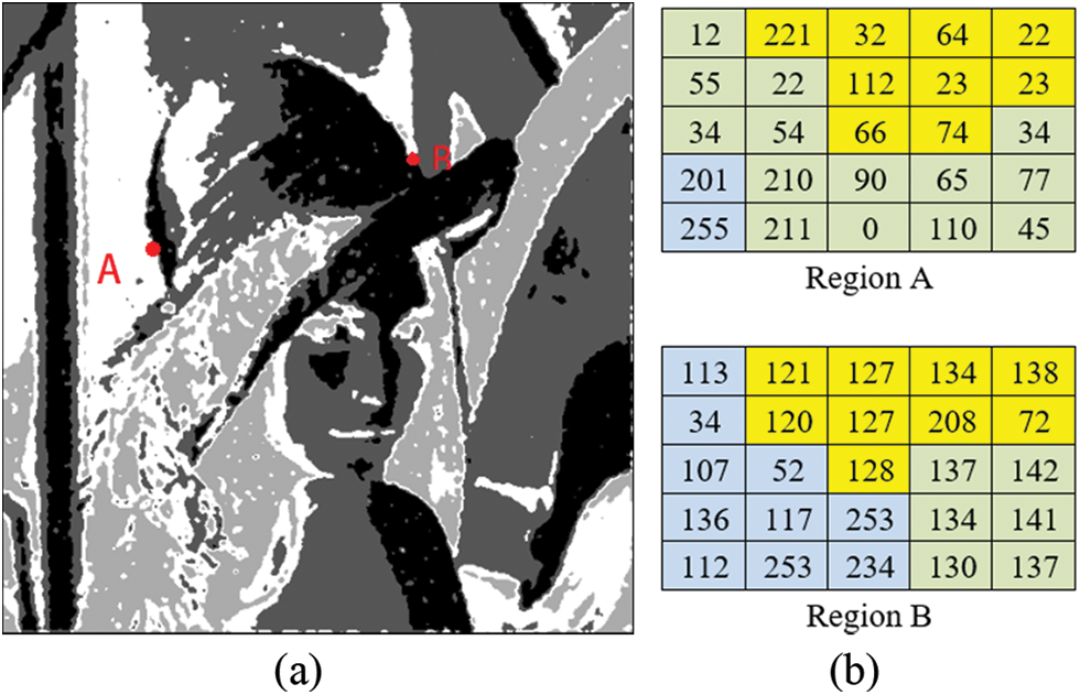
Figure 2: (a) The effect of Lena image clustering with a noise level of 50% when K = 4, (b) The pixel classification result of regions A and B, where the pixels marked blue, green, and yellow indicate that they belong to different kinds
3.2 Determination of Noise Detection Threshold by Iteration
After the pixel clustering operation, the pixels of the image will be clustered into several different clusters according to the similarity of the grayscale distance. Obviously, in different clusters, the corresponding noise detection threshold ranges are also different due to the different gray levels and regions of the pixels. Therefore, it is now necessary to select the optimal detection threshold for different types of pixels. As mentioned in the introduction, for the two-stage denoising algorithm, the better the noise detector, the better the filtering effect, which means that the optimal detection threshold corresponds to the best filtering effect. In other words, the selection of the optimal threshold TLCI for LCI is a process of solving an image-denoising model optimization problem.
Since the LCI value of the pixel is in the range of [0, 1] after normalization, the detection threshold TLCI could be made traverse from 0 to 1 (assuming the step size is 0.1) and calculate the objective function of the model at the same time. When the objective function is the smallest, the corresponding TLCI value is the optimal threshold. The total variational model is often used to solve the optimization problem of image denoising, which mainly relies on the gradient descent method to smooth the image. The paper hope to smooth the image inside the image so that the difference between adjacent pixels is small, and the contour and edge of the image are not smoothed as much as possible [26,27]. Therefore, the paper uses the characteristic that the image belongs to a two-dimensional discrete signal to perform total variation on the image, as shown in Formula (8):
where y is any pixel of the image, i and j are the abscissa and ordinate of y respectively. Since the reason that it is difficult to solve Formula (8), two-dimensional total variation has another commonly used definition of anisotropy:
In Formulas (8) and (9), V(y) is also called the TV norm, which can be used as a regularization method to keep the edge information of the image as the goal. The TV value of the image is the same as the norm of the matrix, and the anisotropy of the image TV is the L1 norm of the matrix, and the isotropic TV of the image is expressed in the same way as the L2 norm of the matrix. Therefore, if the anisotropy V(y) is used as the objective function of the model, the image restoration effect is the best when the V(y) value of the restored image is the smallest. In this way, the method can determine the optimal threshold TLCI of the noise detector.
In Section 3.1, the paper divides the pixels of the image into K categories through the k-means method, and the pixels belonging to the same category are divided into flat areas and complex areas. Therefore, we need to use the iterative method to select the optimal threshold of 2 × K areas, and then calculate the TV value while restoring the image (note that the areas are relatively independent of each other). It is found that with the iteration of the threshold from 0 to 1, the value of V(y) decreases first and then increases. Therefore, there is a threshold to minimize V(y), and the threshold at this time is the optimal threshold we need.
3.3 The Framework of Noise Detection Method
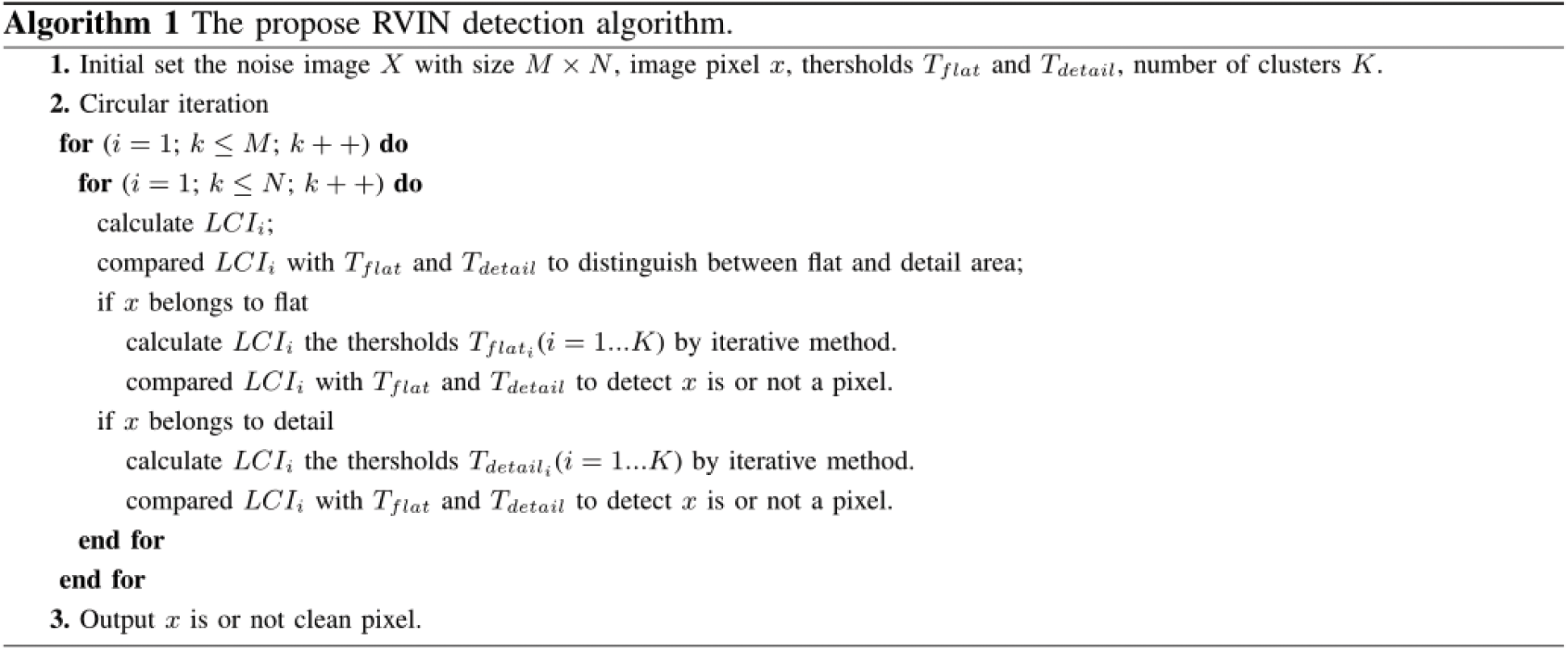
For understanding, the whole framework of the proposed impulse noise detection method is summarized as shown in Algorithm 1:
4 The Proposed Partition Decision Filter
Given the Section 2.2 analysis, it is believed that different filters should be used according to different regions of noise pixels in the filtering stage. In this section, a more robust partition decision filter is designed to remove RVIN instead of using the existing median or improved median filter. The proposed partition decision filter considers the image features and the region of noise at the same time and only selects the pixels judged to be normal in the neighborhood of the central pixel to filter the central pixel.
For the noise pixels judged to be in a flat area, LCI weighted mean filter is designed to repair it. The LCI weighting filter is shown in Formula (10):
where I’x represents the gray value of the noise pixel x after filtering represents the pixel in Ω0x that is judged as clean noise in the noise detection stage, Iy and LCIy represent the gray value and LCI value of y, respectively. The LCI value of the pixel is used as the weight of each pixel in the filter because LCI represents the probability that the pixel is clean. If the larger the LCI value of the pixel, it indicates that it is more likely to be a clean pixel, then it should be given more weight to participate in the repair of the central noise pixel. Considering that the gray distribution of pixels in the flat area is smooth, and if the window setting of the filter is too large, it is easy to introduce pixels in the edge area. Therefore, the filter window of the LCI weighted filter is set to 5 × 5.
For the noise pixels in the edge and detail areas, the gray level of the pixels in the neighborhood changes sharply. However, due to the characteristics of the edge, there will always be pixels in a certain direction in the neighborhood, and the gray difference is small. Therefore, a median filter based on minimum gradient difference is designed, which is named the edge direction filter. The principal steps are summarized as follows:
(1) For the noise pixel x determined to be in the edge or detail area, an M × M detection frame is constructed with the pixel x as the center.
(2) According to the noise results of the first stage, select the clean pixels on the four lines of the detection frame, and put the pixels judged as clean noise on the row, column, left diagonal and right diagonal of the current central pixel x into the set Dh, Dv, Dl and Dr respectively.
(3) Calculate the standard deviation of elements in each set, and select the direction represented by the set with the smallest standard deviation as the boundary filtering direction Df.
(4) The gray values of the clean pixels in the boundary direction are arranged in ascending order, and the median in the election sequence is used as the new gray value of the central noise pixel x.
For understanding the edge direction filter, an edge region from Fig. 3a is selected and the pixel gray distribution corresponding to this region is shown in Fig. 3b. The elements in the four direction set of this region are Dh= [56,95,211], Dv= [82,85,99,106,107], Dl= [80,90,215] and Dr= [38,54,67,117,147], respectively. By calculating the standard deviation of each set, it can be seen that the Dv direction is the edge direction line. From Fig. 3b, it also can be found that the direction of the edge line observed visually is consistent with the direction of the edge line calculated through the method. Then, after median filtering, the gray value of the central pixel is (99) in the Dv set, which is very close to the ground truth (93) of this pixel.
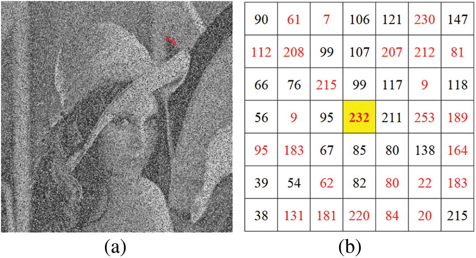
Figure 3: (a) Image of Lena with 50% RVIN, marked with the edge region A whose intensities is listed on the right (b), and the noise pixels are indicated in red color
It should be pointed out that if the window of the filter is too small, there may be few clean pixels in the edge direction, which makes the image prone to burrs and affects the filtering effect. Therefore, the window of the improved median filter is set to 7 × 7 in this paper.
4.3 The Framework of the Filtering Method
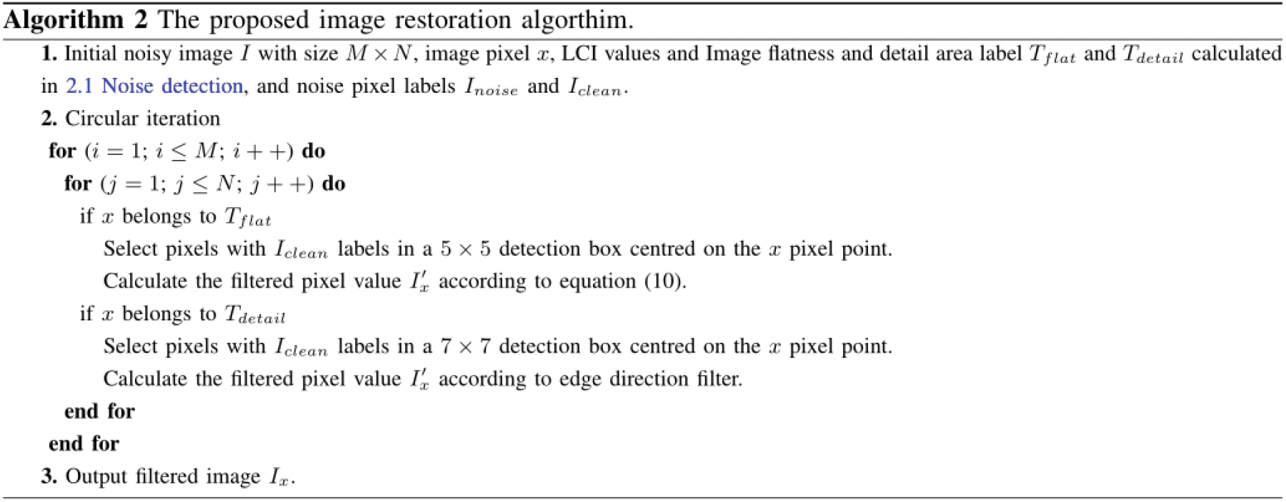
For understanding, the whole framework of the proposed RVIN removal method is summarized as shown in Algorithm 2:
In this section, the noise detection and removal experiments are performed on natural images and medicals image to verify the performance of the proposed method. The test images are shown in Fig. 4, where Figs. 4a–4g are natural images, Figs. 4h–4i are medical images. All image sizes are 512 × 512, except that of the size of House. To quantitatively and qualitatively evaluate the performance and effect of the proposed two-stage denoising algorithm, this paper use the Miss Detected pixels (MD) and False Detected pixels (FD) indexes commonly used in other literature to evaluate the noise detector, and Structural Similarity (SSIM) and Peak Signal to Noise Ratio (PSNR) indexes to evaluate the filter.
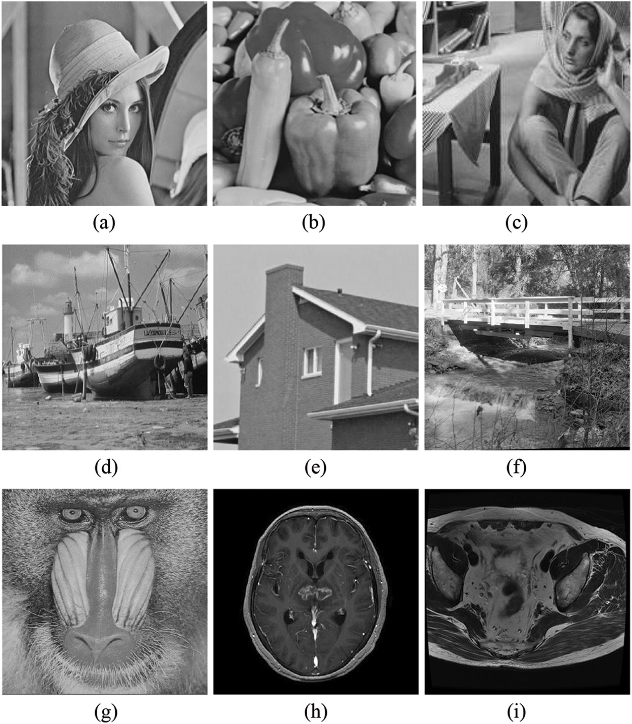
Figure 4: The test images: (a) Lena, (b) Peppers, (c) Barbara, (d) Boat, (e) House, (f) Bridge, (g) Baboon, (h) Gehirn, (i) Prostate
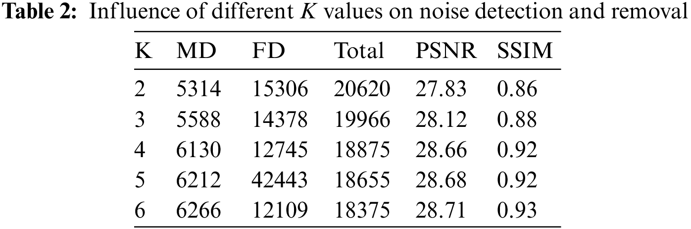
Although the proposed filter is improved based on LCI noise detector, it reduces many unnecessary parameters than the original method. For the parameters in Formula (1), both σλ and σs are taken as 7.1. For the parameter Tσ used to judge whether the noise pixel is in the detail or texture area, the paper follow the settings of the literature [13]. As for the clustering grouping parameter K, it is obvious that the more groups of the damaged image, the better the noise detection effect, which will increase the time cost and complexity of the algorithm at the same time. We select Peppers image with 50% RVIN and divide the pixels into 2~6 groups to verify the impact of the number of groups on noise detection. The experimental data are shown in Table 2. It can be found that when the value of K equals to 4, all indicators basically reach the best. Therefore, the value of K is set to 4 in the later experiments.
5.2 Performance of Proposed Noise Detector
As mentioned in the introduction, the detection accuracy of the noise detector has a great impact on the noise removal ability of the filter. A good noise detector should have fewer missed detected (MD) pixels, false detected (FD) pixels and higher accuracy of real detected noise pixels (True Hit). Table 3 and Fig. 5 show the detection effects of the proposed noise detector on test images with different noise levels. It can be seen from Table 3 that for some images with less texture and simple pixel gray distribution such as Lena, Peppers, Prostate and Brain images, the effect will be better and the number of MD and FD is much less than other images, which was caused by the reason the noise pixels in the flat area are easier to detect than those in the edge area. Although the images of Baboon, Barbara, Boat, and Bridge, which contain more details and textures, perform worse at low noise levels, it can be seen from Fig. 5 that with the increase of noise level, the detection rate of noise pixels in the image is gradually increasing. This is because the improvement of noise level leads to fewer clean pixels in the image and a greater difference in pixel gray distribution in the detection window. At this time, if the central pixel is noisy, it will be easier to be detected since the reason that it is more different from the pixels in its neighborhood. It is worth noting that when the noise level reaches 80%, the truth hit of almost all images is more than 90%, which shows that the proposed noise detector has good stability and robustness.
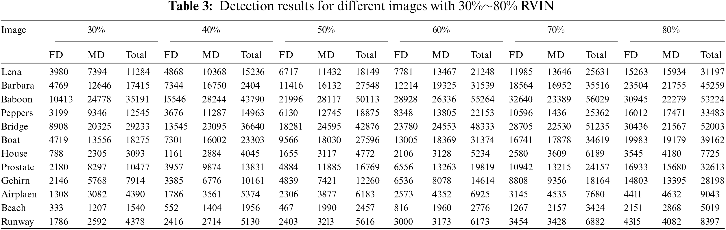
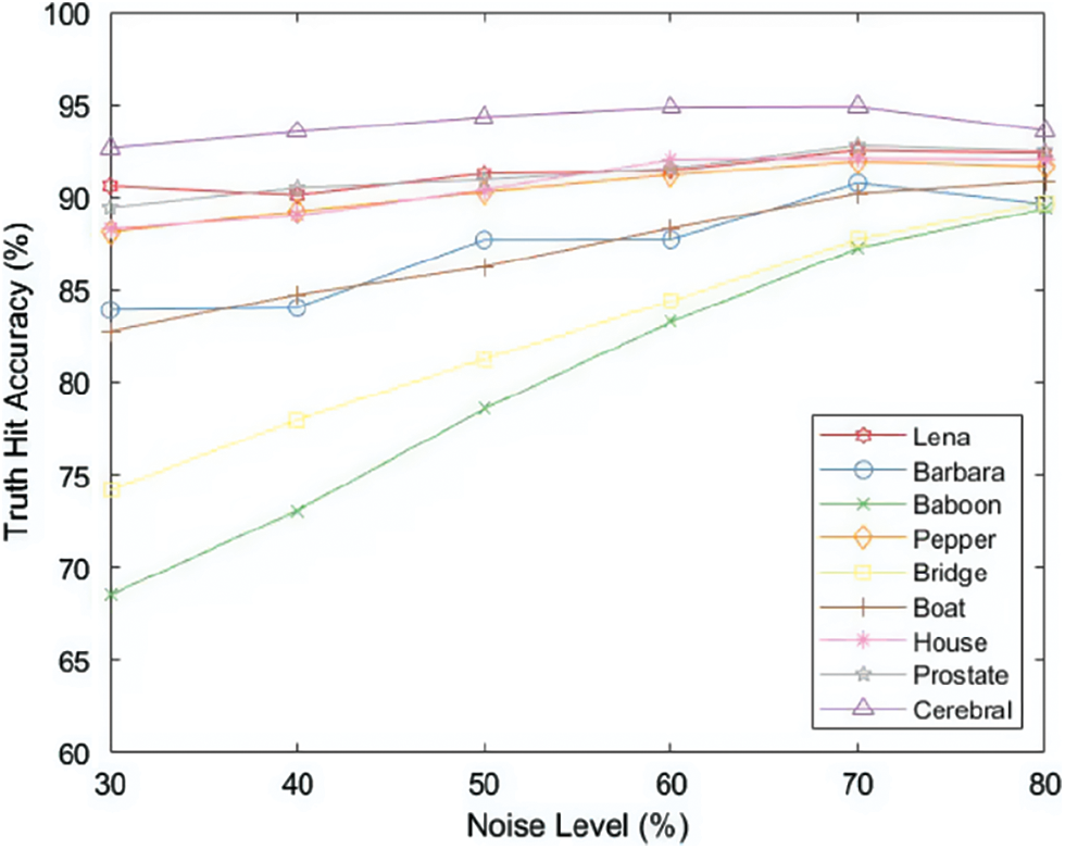
Figure 5: The true hit accuracy for different images with 30%~80% RVIN
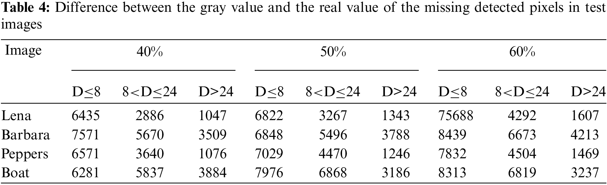
Generally, for gray-scale images, it is not obvious that if the absolute difference between the pixel value and its adjacent pixel value is less than 8 [10,28]. In other words, it is difficult for human eyes or noise detectors to distinguish when the difference between the gray value of noise pixels and their original true value is within 8, and their existence will not significantly reduce the image quality. Therefore, for this part of noise pixels, they can be regarded as clean pixels. Based on this premise, the difference between the gray value and the real value of the missing detected pixels in the test image are counted, as shown in Table 4, where D represents the difference between the current value and the real value of the noise pixel. It can be seen from Table 4 that the gray values of most of the missing noise pixels in these images with 40%~60% RVIN are within 8 bits of their true values, which further verifies that the proposed noise detector has a high noise detection accuracy.
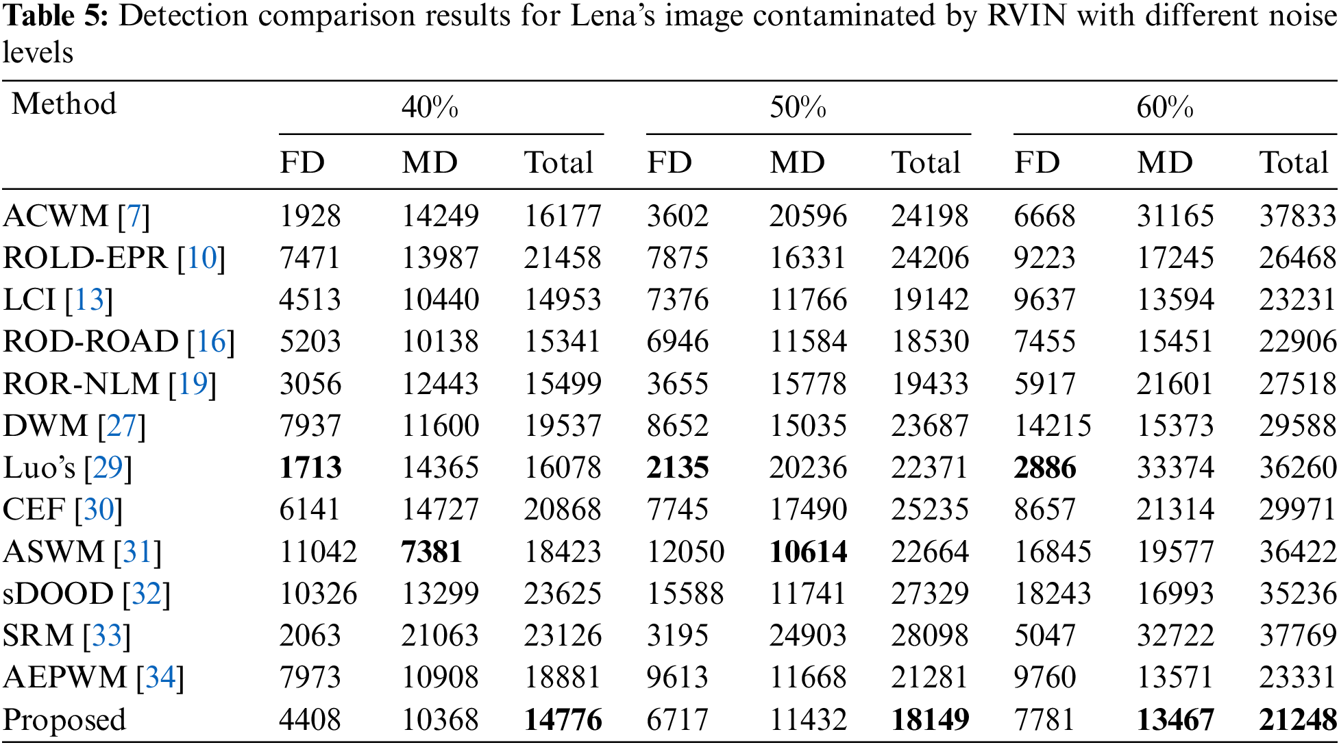
To objectively evaluate the performance of the proposed noise detector, it was compared with several newly proposed and classical algorithms, such as DWM [27], Luo’s method [29], Contrast Enhancement-based Filter (CEF) [30], Adaptive Switching Median (ASWM) method [31], Standard Deviation Obtaining Optimal Direction (SDOOD) method [32], Sparse Regularization Method (SRM) [33], Adaptive Edge Preserving Weighted Mean (AEPWM) method [34] and so on. The experimental results are shown in Table 5. It should be pointed out that for the FD and MD values of other noise detection algorithms, the best values mentioned in the literature are selected. It can be found from Table 5 that although some methods such as Luo’s have a very low number of FD, the number of missed pixels is very high, which will lead to more burrs in the image and affect the recovery performance of subsequent filters. Although the proposed noise detector has a relatively large number of false detected pixels, the total number is optimal under different noise levels. In fact, with the increase of noise level, the MD of proposed detector gradually achieves the optimal result, which means that our method owns better robust, and the detector can still detect more noise pixels even though the noise density becomes higher. Intuitively, a good noise detector should be able to detect more noise pixels while reducing mis-judgment as much as possible. Therefore, considering several evaluation indexes, it is believed that the proposed noise detector has better performance than other methods. In addition, from the comparison results between LCI and the proposed filter, it can also be found that with the increase of noise level, the effect gap between the proposed filter and LCI is more obvious, which shows that the improvement proposed for LCI has an obvious and substantial improvement in detection performance.
5.3 Restoration Performance of Proposed Filter on Natural Image
To verify the effectiveness and rationality of the proposed partition decision filter, restoration experiments are performed on Lena images with 50% RVIN, as shown in Figs. 6a–6b. At the same time, a flat region A and a detail region B with 12 × 12 size are selected from the image, and the corresponding pixel gray values before and after filtering are shown in Figs. 6c–6f. By enlarging Fig. 6b, it can be found that the image has no obvious burr or residual noise mass, which is due to the good detection of noise in the damaged image by the proposed noise detector. As we mentioned earlier in Table 4, although 6800 noise pixels were not detected, half of the gray values of the noise had little difference from the original values, resulting in no obvious visual observation.
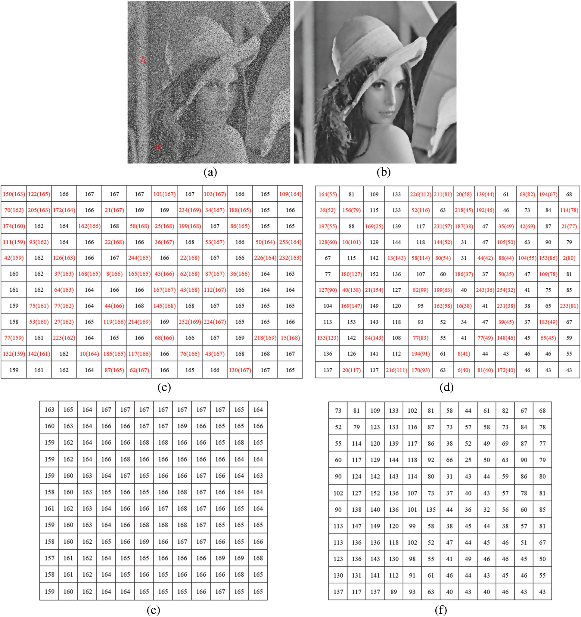
Figure 6: (a) Lena image with 50% RVIN, (b) restored Lena image, (c)–(d) pixel gray distribution of flat region A and detail region B before filtering, in which the pixels marked in red are noise, and the values in brackets are their real values, (e)–(f) pixel gray distribution of flat region A and detail region B after filtering
From the comparison of Figs. 6c–6f, it can be seen that most noise pixels are figured out in both flat and detail areas, and the restored pixel gray values are very close to the real values. For some clean pixels that are judged as noise, the new values are also less different from the original values after being filtered. It is worth noting that the detection and filtering effects of the detail region are significantly inferior to that of the flat region. For example, in the filtered flat region A, there are 144 pixels with the error between the new gray value and the real value within ±3, while there are 37 pixels in the detail area B above ±8. This is because the pixel gray distribution of edge and texture details is more complex, but from the recovery effect of Fig. 6b, the proposed filter still retains and restores the texture and edge with no obvious image blur, which shows the rationality and effectiveness of the sub-regional filtering method.
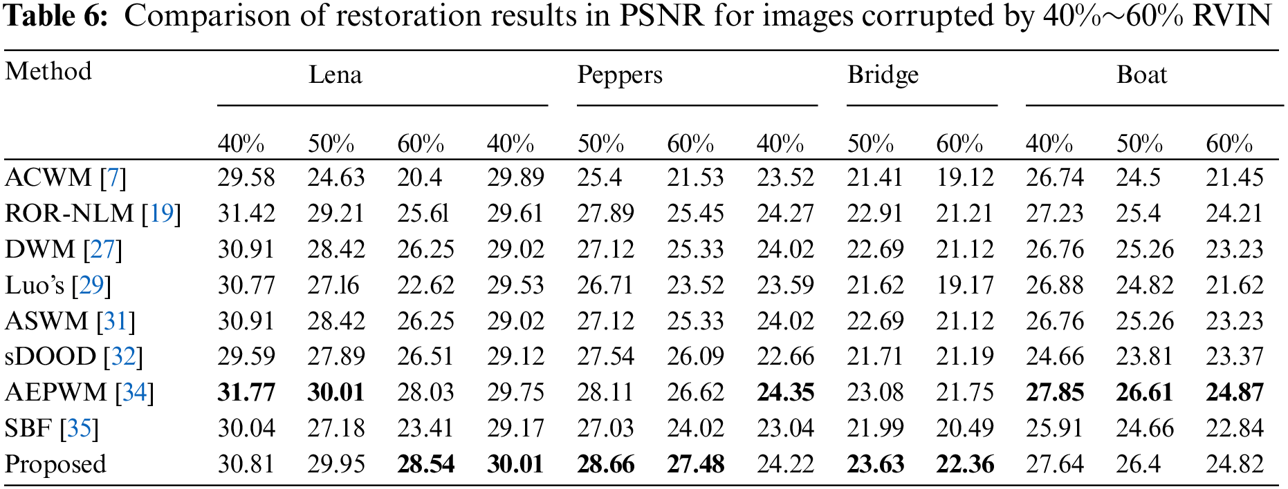
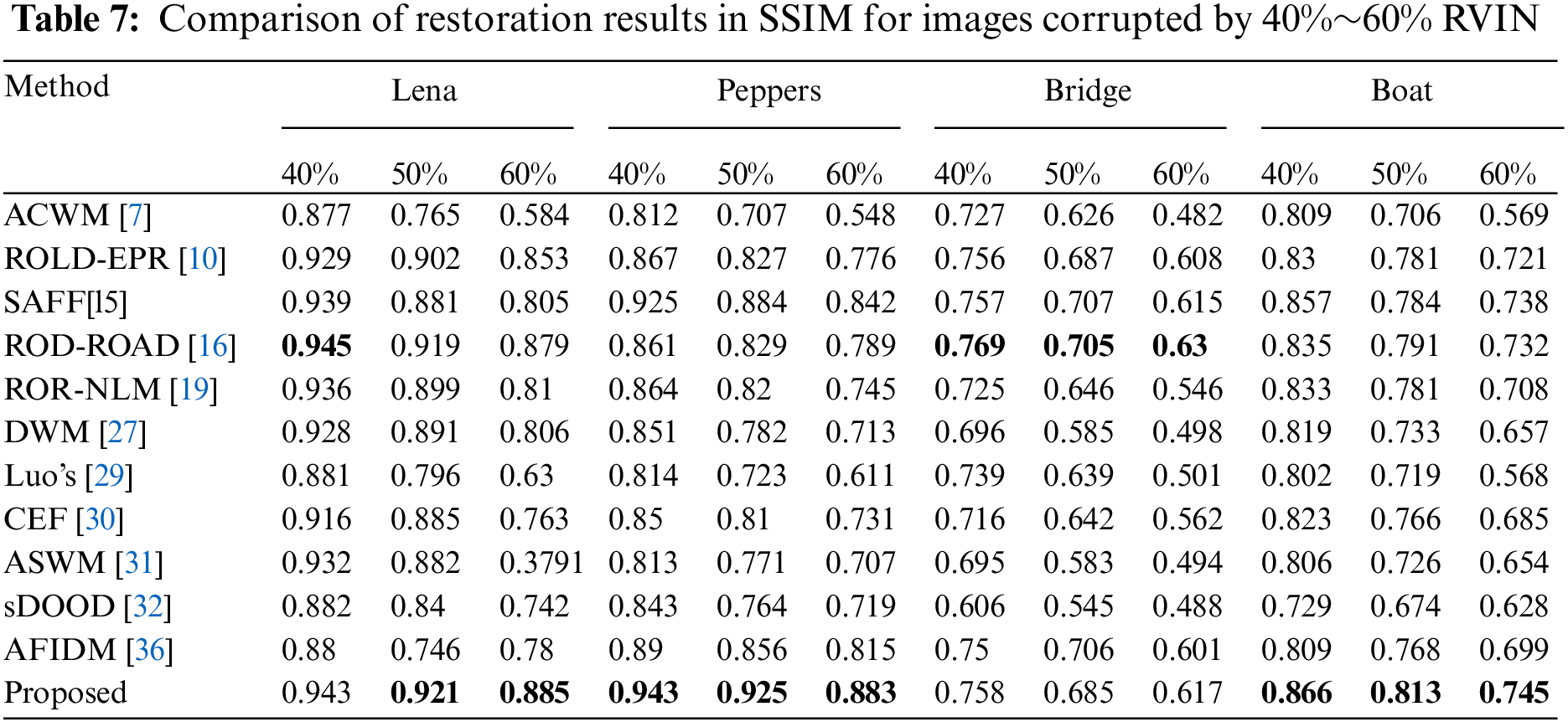
To objectively evaluate the performance of the proposed filter, it was compared with several mainstream filters, such as DWM [27], Luo’s [29], ASWM [31], SDOOD [32], AEPWM [34], Switching Bilateral Filter (SBF) [35], Adaptive Fuzzy Inference Directional Median (AFIDM) method [36] and so on. PSNR indicator is used to measure the similarities and differences between the original image and the reconstructed image, and the SSIM indicator is used to characterize the ability of the filter to pay attention to details and preserve features. For the PSNR and SSIM values of other filters, we select the best values mentioned in their respective literature. From the PSNR comparison results in Table 6, it can be found that the proposed filter is slightly inferior to AEPWM except for the boat image, but the performance of the proposed filter is more prominent in other images, especially at the noise level of 50%~60%. Meanwhile, in the increase of noise level, the PSNR value of the proposed filter decays more slowly than that of AEPWM and other filters, which is because the designed noise detector can detect more noise at high noise levels. In the SSIM comparison results in Table 7, except that the bridge image is slightly lower than ROD-ROAD, the performance of the proposed filter on other images is significantly better than other filtering algorithms, which shows that the proposed filter can better retain the edges and other details in the image.
Similarly, several mainstream filtering algorithms are selected to compare the effect of the filter on the visual output. As shown in Fig. 7, it can be found that there are still many obvious noise images in [27,35,37] and [38], while the restored image of [35] has obvious blur. The effects of [12] and [19] are relatively better, but some edges and details are not well-preserved. In contrast, the effect of the proposed filter has better visual quality. By enlarging some detail areas in the image such as the places marked in Fig. 7, it can be found that the proposed method retains the lines and colors of the hull better than other methods, which is due to the high detection accuracy of the noise detector and the zoning filtering design of the filter. It can be considered that for complex images with 60% RVIN, the proposed method can still detect and remove most of the random-value impulse noise and retain most of the image details.
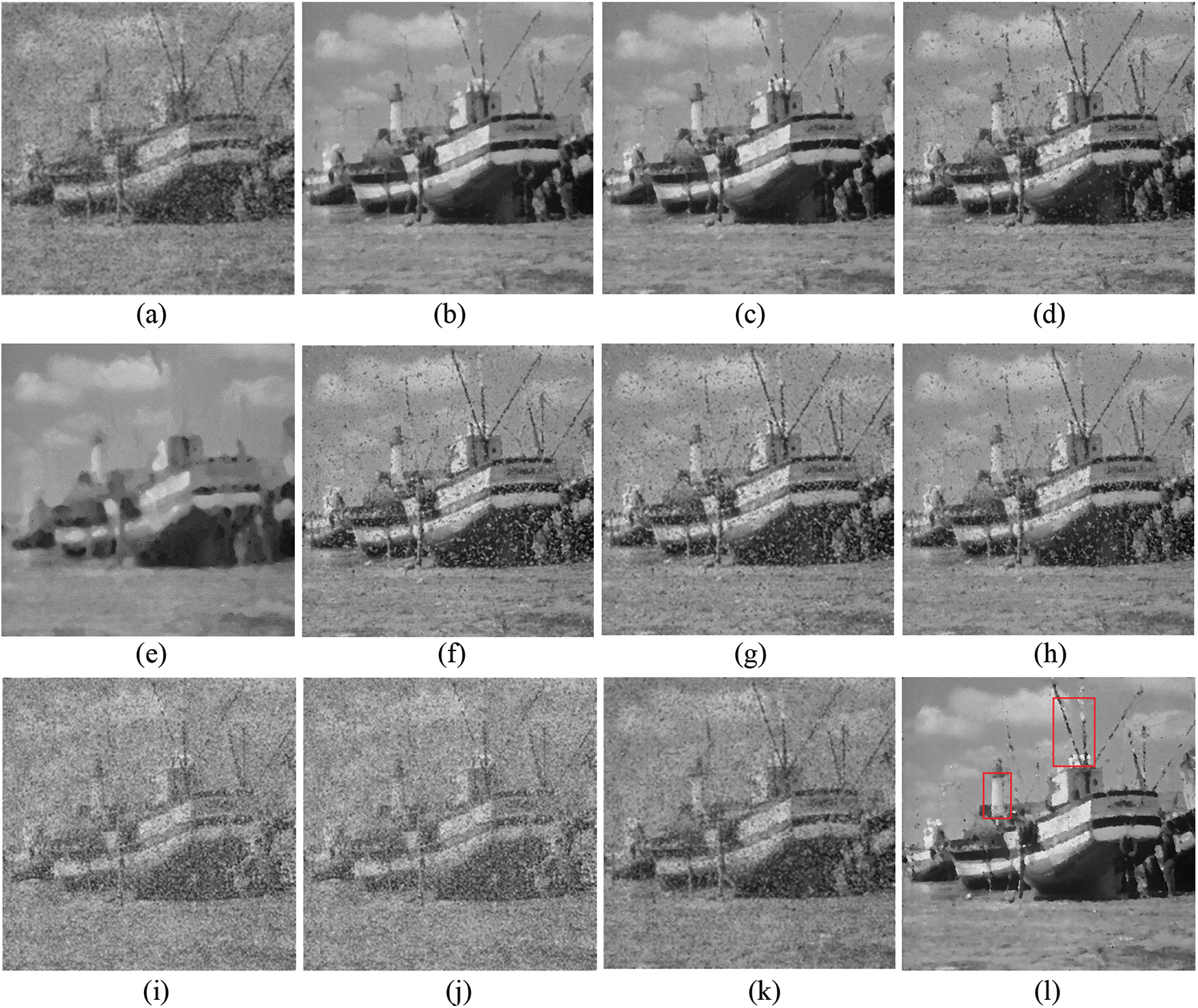
Figure 7: Restoration results of Boat images with 60% RVIN: (a) Boat with 60% RVIN, (b) AFWMF [12], (c) ROR [19], (d) DWM [27], (e) SDOOD [32], (f) SBF [35], (g) EAIF [37], (h) ASMF [38], (i) FRDFN [39], (j) EBDND [40], (k) BDND [41], (l) Proposed filter
5.4 Restoration Performance on Medical Image
Denoising experiments on medical images were conducted as shown in Fig. 8. It can be seen that the denoising algorithm proposed in this paper can restore biomedical images with different textures and resolutions under different levels of RVIN. From the restored medical image, it also can be intuitively observed that the algorithm in this paper also has a good texture and edge preservation ability in a medical image, which helps to ensure the correct diagnosis and treatment in the follow-up. In general image processing, small details have little impact on the subsequent processing procedures of image noise reduction. However, such small mistakes are not allowed when the processing object is medical images, because, in medical diagnosis or treatment, every small mistake will affect the treatment methods and even threaten the life of the patient.
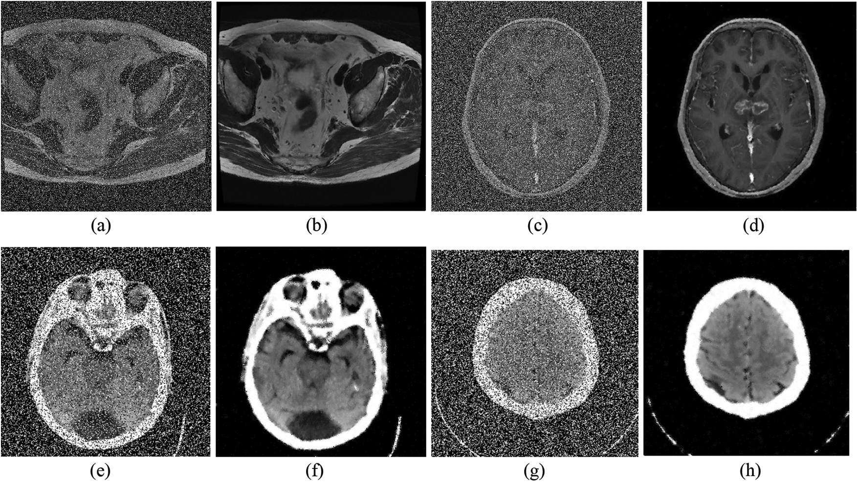
Figure 8: The filtering effects of the proposed method on Prostate and Gehirn noisy images: (a) Prostate with 30% RVIN; (b) restored image of (a), PSNR = 31.82; (c) Gehirn with 50% RVIN; (d) restored image of (c), PSNR = 29.76; (e) Brain with 40% RVIN; (f) restored image of (e), PSNR = 22.47; (g) Cross section of brain with 50% RVIN; (h) restored image of (g), PSNR = 23.26
5.5 Comparison of Computation Cost
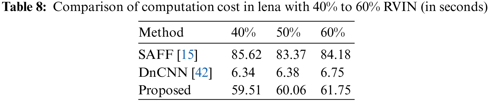
The proposed method was compared with the best algorithms SAFF and DnCNN in traditional methods and deep learning methods, as shown in Table 8. Both the method proposed in this paper and SAFF are two-stage RVIN removal methods, but the calculation speed of the proposed method is more than 20 s faster than that of SAFF. It should be pointed out that DnCNN is an end-to-end one-stage denoising method. For the trained denoising model, it can directly skip the noise detection phase to complete the noise removal, so it only takes about 6 seconds. The calculation time of the proposed method is mostly in the noise detection stage. If only the filtering stage is considered, the proposed method only takes about 3 seconds to remove RVIN from Lena’s image. To sum up, the proposed method has obvious advantages in the execution time in the noise detection stage and the removal stage, which provides more convenience for the implementation of the algorithm.
In this paper, a novel two-stage method to remove random-value impulse noise is present. In the noise detection stage, all pixels in the damaged image are divided into several groups according to the characteristics of pixels, and then the noise of each group of pixels is recognized by adaptive threshold. For the noisy pixels in flat area and detail area, LCI weighted filter and edge direction median filter are designed to recover the gray value of the noisy pixels respectively. Large number of experimental results show that the proposed method is suitable for RVIN in natural images or medical images, and the performance of the algorithm is more robust and stable with the increase of noise level.
Although the proposed filter is slightly inferior to some advanced one-stage filters in PSNR, it is essentially superior to other denoising methods in SSIM and visual quality evaluation. In future work, we will further research how to increase the accuracy of noise detection and improve the filtering performance. Meanwhile, the feasibility of applying the proposed method to color images, hyperspectral data, and textual data can also be further discussed.
Funding Statement: This work is supported by the Hainan Provincial Natural Science Foundation of China (621MS019), Major Science and Technology Project of Haikou (Grant: 2020-009), Innovative Research Project of Postgraduates in Hainan Province (Qhyb2021-10), National Natural Science Foundation of China(Grant: 62062030) and Key R&D Project of Hainan province (Grant: ZDYF2021SHFZ243).
Conflicts of Interest: The authors declare that they have no conflicts of interest to report regarding the present study.
References
1. Y. Wu and S. Li, “A novel fusion paradigm for multi-channel image denoising,” Information Fusion, vol. 77, no. 8, pp. 62–69, 2022. [Google Scholar]
2. L. Afraites, A. Hadri, A. Laghrib and M. Nachaoui, “A weighted parameter identification pde-constrained optimization for inverse image denoising problem,” The Visual Computer, vol. 38, no. 8, pp. 2883–2898, 2022. [Google Scholar]
3. W. Dong, P. Wang, W. Yin, G. Shi, F. Wu et al., “Denoising prior driven deep neural network for image restoration,” IEEE Transactions On Pattern Analysis and Machine Intelligence, vol. 41, no. 10, pp. 2305–2318, 2018. [Google Scholar] [PubMed]
4. S. Rawat, K. Rana and V. Kumar, “A novel complex-valued convolutional neural network for medical image denoising,” Biomedical Signal Processing and Control, vol. 69, pp. 102859, 2021. [Google Scholar]
5. H. Hwang and R. A. Haddad, “Adaptive median filters: New algorithms and results,” IEEE Transactions On Image Processing, vol. 4, no. 4, pp. 499–502, 1995. [Google Scholar] [PubMed]
6. T. Chen and H. R. Wu, “Adaptive impulse detection using centerweighted median filters,” IEEE Signal Processing Letters, vol. 8, no. 1, pp. 1–3, 2001. [Google Scholar]
7. T. C. Lin, “A new adaptive center weighted median filter for suppressing impulsive noise in images,” Information Sciences, vol. 177, no. 4, pp. 1073–1087, 2007. [Google Scholar]
8. N. Singh, T. Thilagavathy, T. Ramasubramanian and O. Umamaheswari, “Some studies on detection and filtering algorithms for the removal of random valued impulse noise,” IET Image processing, vol. 11, no. 11, pp. 953–963, 2017. [Google Scholar]
9. R. Garnett, T. Huegerich and C. Chui, “A universal noise removal algorithm with an impulse detector,” IEEE Transactions on Image Processing, vol. 14, no. 11, pp. 1747–1754, 2005. [Google Scholar] [PubMed]
10. Y. Dong, R. H. Chan and S. Xu, “A detection statistic for random-valued impulse noise,” IEEE Transactions on Image Processing, vol. 16, no. 4, pp. 1112–1120, 2007. [Google Scholar] [PubMed]
11. Q. Chen, M. Huang, H. Wang and G. Xu, “A feature discretization method based on fuzzy rough sets for high-resolution remote sensing big data under linear spectral model,” IEEE Transactions on Fuzzy Systems, vol. 30, no. 5, pp. 1328–1342, 2022. [Google Scholar]
12. J. R. Chang, Y. Chen, C. Lo and H. Chen, “An advanced AFWMF model for identifying high random-V alued impulse noise for image processing,” Applied Sciences, vol. 11, no. 15, pp. 7021–7037, 2021. [Google Scholar]
13. X. Xiao, N. Xiong, J. H. Lai, C. Wang, Z. Sun et al., “A local consensus index scheme for random-valued impulse noise detection systems,” IEEE Transactions on Systems, Man, and Cybernetics: Systems, vol. 51, no. 6, pp. 3412–3428, 2019. [Google Scholar]
14. N. Singh and U. Oorkavalan, “Triple threshold statistical detection filter for removing high density random-valued impulse noise in images,” EURASIP Journal on Image and Video Processing, vol. 2018, no. 1, pp. 1–16, 2018. [Google Scholar]
15. M. Nadeem, A. Hussain, A. Munir, M. Habib and M. T. Naseem, “Removal of random valued impulse noise from grayscale images using quadrant based spatially adaptive fuzzy filter,” Signal Processing, vol. 169, pp. 107403, 2020. [Google Scholar]
16. L. Liu, C. P. Chen, Y. Zhou and X. You, “A new weighted mean filter with a two-phase detector for removing impulse noise,” Information Sciences, vol. 315, no. 6, pp. 1–16, 2015. [Google Scholar]
17. P. Civicioglu, “Removal of random-valued impulsive noise from corrupted images,” IEEE Transactions On Consumer Electronics, vol. 55, no. 4, pp. 2097–2104, 2009. [Google Scholar]
18. X. Lan and Z. Zuo, “Random-valued impulse noise removal by the adaptive switching median detectors and detail-preserving regularization,” Optik, vol. 125, no. 3, pp. 1101–1105, 2014. [Google Scholar]
19. B. Xiong and Z. Yin, “A universal denoising framework with a new impulse detector and nonlocal means,” IEEE Transactions on Image Process, vol. 21, no. 4, pp. 1663–1675, 2012. [Google Scholar]
20. C. Tomasi and R. Manduchi, “Bilateral filtering for gray and color images,” in Sixth Int. Conf. on Computer Vision, Bombay, India, pp. 839–846, 1998. [Google Scholar]
21. C. C. Kang and W. J. Wang, “Fuzzy reasoning-based directional median filter design,” Signal Processing, vol. 89, no. 3, pp. 344–351, 2009. [Google Scholar]
22. X. Wang, X. Q. Zhao, F. X. Guo and J. F. Ma, “Impulsive noise detection by double noise detector and removal using adaptive neural-fuzzy inference system,” AEU-International Journal of Electronics and Communications, vol. 65, no. 5, pp. 429–434, 2011. [Google Scholar]
23. R. Kosarevych, O. Lutsyk and B. Rusyn, “Detection of pixels corrupted by impulse noise using random point patterns,” The Visual Computer, vol. 6, pp. 1–12, 2021. [Google Scholar]
24. J. Revaud, P. Weinzaepfel and Z. Harchaoui, “Epicflow: Edge-preserving interpolation of correspondences for optical flow,” in IEEE Int. Conf. on Computer Vision and Pattern Recognition (CVPR), Boston, Massachusetts, USA, pp. 1164–1172, 2015. [Google Scholar]
25. A. Criminisi, T. Sharp, C. Rother and P. P. E. Rez, “Geodesic image and video editing,” Acm Transactions On Graphics, vol. 29, no. 5, pp. 131–134, 2010. [Google Scholar]
26. Y. Chen and Y. Gao, “Image denoising via steerable directional Laplacian regularizer,” Circuits Syst. Signal Process, vol. 40, no. 12, pp. 6265–6283, 2021. [Google Scholar]
27. Y. Dong and S. Xu, “A new directional weighted median filter for removal of random-valued impulse noise,” IEEE Signal Processing Letters, vol. 14, no. 3, pp. 193–196, 2007. [Google Scholar]
28. Q. Chen, M. Huang and H. Wang, “A feature discretization method for classification of high-resolution remote sensing images in coastal areas,” IEEE Transactions on Geoscience and Remote Sensing, vol. 59, no. 10, pp. 8584–8598, 2021. [Google Scholar]
29. W. Luo, “A new efficient impulse detection algorithm for the removal of impulse noise,” IEICE Transactions on Fundamentals of Electronics, Communications and Computer Sciences, vol. 88, no. 10, pp. 2579–2586, 2005. [Google Scholar]
30. U. Ghanekar, A. K. Singh and R. Pandey, “A contrast enhancement-based filter for removal of random valued impulse noise,” IEEE Signal Processing Letters, vol. 17, no. 1, pp. 47–50, 2010. [Google Scholar]
31. S. Akkoul, R. Ledee, R. Leconge and R. Harba, “A new adaptive switching median filter,” IEEE Signal Processing Letters, vol. 17, no. 6, pp. 587–590, 2010. [Google Scholar]
32. A. S. Awad, “Standard deviation for obtaining the optimal direction in the removal of impulse noise,” IEEE Signal Processing Letters, vol. 18, no. 7, pp. 407–410, 2011. [Google Scholar]
33. B. Deka, M. Handique and S. Datta, “Sparse regularization method for the detection and removal of random-valued impulse noise,” Multimedia Tools and Applications, vol. 76, no. 5, pp. 6355–6388, 2017. [Google Scholar]
34. N. Iqbal, S. Ali, I. Khan and B. M. Lee, “Adaptive edge preserving weighted mean filter for removing random-valued impulse noise,” Symmetry-Culture and Science, vol. 11, no. 3, pp. 395, 2019. [Google Scholar]
35. C. H. Lin, J. S. Tsai and C. T. Chiu, “Switching bilateral filter with a texture/noise detector for universal noise removal,” IEEE Transactions on Image Processing A Publication of the IEEE Signal Processing Society, vol. 19, no. 9, pp. 2301–2307, 2010. [Google Scholar]
36. M. Habib, A. Hussain, S. Rasheed and M. Ali, “Adaptive fuzzy inference system based directional median filter for impulse noise removal,” AEU-International Journal of Electronics and Communications, vol. 77, no. 5, pp. 689C–697, 2016. [Google Scholar]
37. W. Luo, “An efficient algorithm for the removal of impulse noise from corrupted images,” AEU-International Journal of Electronics and Communications, vol. 61, no. 8, pp. 551–555, 2007. [Google Scholar]
38. P. J. S. Sohi, N. Sharma, B. Garg and K. V. Arya, “Noise density range sensitive mean-median filter for impulse noise removal,” in Innovations in Computational Intelligence and Computer Vision. Vol. 1189. Springer, pp. 150–162, 2021. [Google Scholar]
39. C. C. Kang and W. J. Wang, “Fuzzy reasoning-based directional median filter design,” Signal Processing, vol. 89, no. 3, pp. 344–351, 2009. [Google Scholar]
40. I. F. Jafar, R. A. AlNamneh and K. A. Darabkh, “Efficient improvements on the BDND filtering algorithm for the removal of highdensity impulse noise,” IEEE Transactions on Image Processing, vol. 22, no. 3, pp. 1223–1232, 2013. [Google Scholar] [PubMed]
41. P. E. Ng and K. K. Ma, “A switching median filter with boundary discriminative noise detection for extremely corrupted images,” IEEE Transactions on Image Processing, vol. 15, no. 6, pp. 1506–1516, 2006. [Google Scholar] [PubMed]
42. K. Zhang, W. Zuo, Y. Chen, D. Meng and L. Zhang, “Beyond a gaussian denoiser: Residual learning of deep CNN for image denoising,” IEEE Transactions On Image Processing, vol. 26, no. 7, pp. 3142–3155, 2017. [Google Scholar] [PubMed]
Cite This Article
 Copyright © 2023 The Author(s). Published by Tech Science Press.
This work is licensed under a Creative Commons Attribution 4.0 International License , which permits unrestricted use, distribution, and reproduction in any medium, provided the original work is properly cited.
 Downloads
 Citation Tools