Parameter Tuned Deep Learning Based Traffic Critical Prediction Model on Remote Sensing Imaging

1  Introduction

Vehicle traffic assessment and monitoring had a great contribution to road safety. For instance, congestion detection and automatic traffic counting systems will help improve traffic flow planning [1]. Minimizing congestion and formulating traffic accident prediction methods aid in avoiding severe injuries and collisions. Tools for pavement condition evaluation present rapid access to road condition data, which will be helpful for traffic planners to frame a special assessment and monitoring mechanism. Traffic noise prediction and vehicle emission detection effectively minimise pollution [2]. Real-time and near-real-time data on traffic counts, road conditions, and road environment features were crucial for traffic assessment and monitoring [3]. Ground-related data acquisition sensors (i.e., noise level meters, pneumatic tubes, magnetic sensors, vehicle emission meters, video detection systems, and inductive loop detectors) are to fail and were expensive to install and maintain in certain nations. Alternative technologies, like remote sensing (RS), could offer cheaper solutions for road traffic data acquisition [4]. But in certain cases, both techniques are combined for performing validated assessment and monitoring. Fig. 1 depicts the overview of the traffic prediction system.

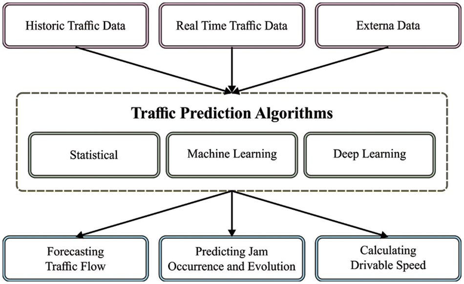
Figure 1: Overview of the traffic prediction system

Recently, the number of research actions relevant to using remote sensing (RS) technologies in their implementation in transportation mechanisms has increased enormously. Transportation systems are considered the basis for all countries’ economic development [5]. Yet, several cities worldwide were encountering an uncontrolled growth in traffic volume, which caused serious issues like increased carbon dioxide (CO2) emissions, delays, higher fuel prices, accidents, traffic jams, emergencies, and degradation in the quality of life of modern society [6]. Advancements in information and communication technology (ICT) in regions like communications, hardware, and software have made novel chances to formulate a sustainable, intellectual transportation mechanism. Incorporating ICT with the transportation structure would allow a better, safe travelling experience and migration to intelligent transportation systems (ITS) that mainly focus on 4 basic principles: responsiveness, sustainability, safety, and integration [7].

The success of ITS is mainly based on the platform utilized for accessing, collecting, and processing precise data from the atmosphere [8]. RS (both satellite and terrestrial) was an appropriate technique to efficiently collect data on a large scale, having an accuracy level that gratifies the ITS demand. Various advanced technologies have allowed automated modeling, and data interpretation was a fascinating topic of RS-related ITS [9]. Spatiotemporal analysis utilizing remote-sensing satellite imageries as an alternative serves a significant role in comprehending the effect of extreme events on a global scale. But such ability was generally limited because of the lack of temporal resolution or spatial resolution of the data; thus, many applications are held on the landscape level, namely for urbanization, water, snow, deforestation, and so on [10]. The recent advancement of satellite constellations (i.e., Planet and Worldview) could offer high spatial resolution images at higher temporal frequency.

This article introduces an Optimal Deep Learning for Traffic Critical Prediction Model on High-Resolution Remote Sensing Images (ODLTCP-HRRSI). The presented ODLTCP-HRRSI technique majorly aims to forecast the critical traffic in smart cities. To attain this, the presented ODLTCP-HRRSI model performs two major processes. At the initial stage, the ODLTCP-HRRSI technique employs a convolutional neural network with an autoencoder (CNN-AE) model for productive and accurate traffic flow. Next, the hyperparameter adjustment of the CNN-AE model is performed via the Bayesian adaptive direct search optimization (BADSO) algorithm. The experimental evaluation of the ODLTCP-HRRSI technique takes place, and the results are assessed under distinct aspects.

The rest of the paper is organized as follows. Section 2 provides related works, Section 3 introduces the proposed model, Section 4 provides result analysis, and Section 5 draws conclusions.

2  Literature Review

Kothai et al. [11] devised a novel boosted long short-term memory ensemble (BLSTME) and convolutional neural network (CNN) method that joint the robust attributes of CNN, including BLSTME, for negotiating the dynamic behavior of vehicles and predicting the overcrowding in traffic efficiently on roads. The CNN will extract the attributes from traffic imageries, and the devised BLSTME strengthens and trains weak techniques for predicting congestion. Wang et al. [12] proposed a Prediction Architecture of a Neural Convolutional Short Long-Term Network (PANCSLTN) for efficiently capturing dynamic non-linear traffic systems with DL assistance. The PANCSLTN could address the issue of backdated decay mistakes through memory blocks and displays better predictive capability for time sequences, including long-time dependency. Patel et al. [13] modelled a new network utilizing deep CNN with long short term memory (LSTM) that derives the features from satellite imageries for land cover classification. The CNN was utilized for deriving the features from these images, and the LSTM network was utilized to support the classification and sequence prediction.

Byun et al. [14] introduce a deep neural network (DNN)-related technique to mechanically predict the vehicle’s speed on roads from videos of drones. This modelled technique includes the following: tracking and detecting vehicles through video analyses, (2) computing the image scales utilizing distances among lanes on the roads, and lastly, predicting the velocity of vehicles. Dai et al. [15] formulate an innovative spatiotemporal deep learning (DL) structure that mainly focuses on providing precise and timely traffic speed prediction. To extract traffic data’s spatial and temporal features concurrently, this structure will combine 2 different DL techniques: the convolutional graph network (GCN) and convolutional LSTM (ConvLSTM). Specifically, the ConvLSTM method can be employed to learn traffic data’s temporal dynamics for deriving temporal features. Conversely, the graph convolutional network (GCN) technique can be employed to learn traffic data’s spatial complexities for extracting spatial features.

In Reference [16], a DNN-related optimization technique can be applied in 2 ways firstly, by utilizing various techniques for activation and training, and secondly, by compiling with feature selecting techniques like a wrapper for feature-subset selection (WFS) approaches and correlation-related feature selection (CFS). Such techniques were compiled to generate traffic noise maps for different times of the day on weekdays, including night, morning, evening, and afternoon. This work mainly focuses on incorporating feature-selecting techniques with the DNN for vehicular traffic noise modelling. Yang et al. [17] devised a novel DL technique called TmS-GCN for forecasting region-level traffic data made up of gated recurrent unit (GRU) and GCN. The GCN part will capture spatial dependence between regions, whereas the GRU part will capture the dynamic traffic change in the regions. Although several models are available in the literature, various hyperparameters have a major influence on the performance of the CNN model. Principally, the hyperparameters such as epoch count, batch size, and learning rate selection are vital to reach effectual outcome. Since the trial and error method for hyperparameter tuning is a tedious and erroneous process, metaheuristic algorithms can be applied. Therefore, in this work, BADSO algorithm can be employed for the parameter selection of the CNN-AE model.

3  The Proposed Model

This article has developed a new ODLTCP-HRRSI technique to forecast critical traffic in smart cities. To attain this, the presented ODLTCP-HRRSI model performs two major processes. At the initial stage, the ODLTCP-HRRSI technique employed the CNN-AE model for productive and accurate traffic flow. Next, the hyperparameter adjustment of the CNN-AE model is performed via the BADSO algorithm.

3.1 Traffic Prediction Module

The ODLTCP-HRRSI technique employed the CNN-AE model for productive and accurate traffic flow in this study. CNN model is mainly designed for handling image recognition and classification processes. It holds the merits of managing high-dimensional data. It comprises convolution and downsampling layers for reducing the reduced dimension of input images and extracting abstract features of the images. In addition, a weight distribution scheme employed in CNN enables the management of high-dimension data by using a few learnable variables and eliminating location sensitivity issues [18]. The CNN-AE is a version of the CNN model, which includes an encoder for extracting features from the input and a decoder, the inverse of the encoder. Besides, CNN enables the reconstruction of the images from the derived features. Owing to the capability of reconstructed data, the CNN-AE model becomes familiar. In the CNN-AE model, the encoding unit has a 3-D convolution layer (CL) to derive features and undergo a down-sampling process. Every individual CL encompasses many channels equivalent to various features to be learned. The CL embed to a non-linear activation function and bias functioning as given below:

qil=σ(kil⊗ql−1+bil),(1)

where qil denotes the outcome of an ith channel in the l th CL, σ represents the rectified linear unit (ReLU) activation function, kil is the trainable convolution filter, ⊗ the convolutional operator, and bil is the ith bias. Here, χ is a 4×4 input image with zero padding, k implies a 3×3 convolutional kernel (or filter), whereas y is the outcome of the convolutional function. The convolutional window gets traversal via the padded input images in the horizontal and vertical directions, where the convolutional function with the filter can be carried out. The step size of all moves represents the stride. The filter derives input image features during the convolution function, and the learnable weights remain the same as the convolution window traverses. Consequently, the filter weights get distributed by the entire input image. Due to the weight sharing, only one filter with 9 weights is necessary for deriving the feature via the whole padded image—rather than 16 distinct filters equivalent to every output component. Here, the filter is not dependent on the position resulting in less number of learnable weights and, therefore, a highly effective training procedure. The convolution operation comprises an intrinsic product among the convolution window and filter for producing respective output components.

Paddings of zeros will be utilized for controlling the output size as the convolution operation minimizes the size of an image. For example, the output size of the original input image is 4 × 4 (solid boxes in x) was 2×2 (solid boxes in y). But with paddings, the resultant comprises the same size as the original input. Practically, the convolution function could work on 3D and 2D dimensional inputs. As the convolution function includes a linear transformation, an activation function was required to provide the non-linear transformation into the CNN. When a comparison is made to the sigmoid or hyperbolic tangent-activated functions, the ReLU in hidden layers could increase the ML algorithm’s computing efficacy. The ReLU function was given below

σ(θ)=max(0,θ),(2)

whereas θ was the outcome of convolution operation with the linear bias. The decoder has 2 transposed CLs, which can be the inverses of CLs to up-sample the data and build the flow domain. The discrepancy among the targeted values and output at the time of training iterations was computed utilizing the mean square error (MSE) loss functions. After that, the weights in the biases and convolutional filters were upgraded by the backpropagation technique to reduce the loss function. For determining the variables of the CNN structure, that is, the number of channels and layers and the stride and kernel sizes, a sequence of parameter amalgamations can be tested to ensure the highest accuracy of fallouts and a minimal number of learnable variables. The padding size can be sumptuously determined to ensure the correct output sizes. Fig. 2 illustrates the process of the CNN-AE system.

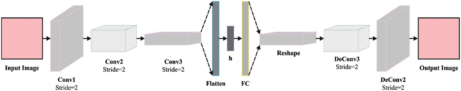
Figure 2: Process of CNN-AE method

3.2 Hyperparameter Tuning Using BADSO Algorithm

To improve the prediction performance, the hyperparameter adjustment of the CNN-AE model is performed via the BADSO algorithm. BADSO is a global local arbitrary searching technique and a hybrid Bayesian optimization (BO) technique that integrates the mesh adaptive direct search (MEADS) with BO search [19]. BADSO alternatives among systematic and sequences of rapid local BO phases (the searching phase of MEADS), slow exploration of mesh grid (poll phase). These two phases complement one another and, during the search process, effectively examine the space and offer an acceptable surrogate method. Once the search process continuously failed, then the genetic programming (GP) method could not assist optimization (because of the excess un- certainty or specified error model), and BADSO switched to the poll phase. Model-free and Fail-safe optimization can be implemented in the poll stage, where BADSO gathers data regarding the local shape of OF for constructing the best proxy for the following search phase. In the study, the sampling point produced during BO is applied as the associate technique of the MEADS for seeking benefits that enhance the success rates of sample point selection and decrease the iteration count in the model. Thus, the BADSO approach could enhance the convergence speed and optimization efficiency.

Search stage

In this phase, a Gaussian model is suitable for the local set of the points computed so far. Next, iteratively selects points to estimate based on the low confidence bounds, which tradeoff among exploitation of potential solution (lower GP mean) and exploration of uncertain region (higher GP uncertainty). The procedure is evaluated using the D mesh direction set and Δkm size parameter; amongst others, the mesh size variable Δkm is utilized to control the search space. Beforehand the k-th iterations, the optimum solution of OF is represented by x, and Sk can describe the determined potential solution. M can describe the set formed by each search point, and the formula can be given below:

Mk={x∈Se}∪{xk+ΔkmDz}(3)

In Eq. (3), z indicates a complete rank positive integer matrixes, z∈Z+p;p represents the amount of direction vector; Z+ denotes the non-negative integer. There exist four stages included in the search phase.

Step 1: Construct grid cell and xk as the searching center.

Step 2: Compute the target values of finite grid-points nearby the constructed grid component and identify potential solutions for improving OF.

Step 3: When a possible solution to enhance the OF is identified, the search becomes effective. Now, shift the grid center to the location and the mesh size variable Δk+1m is raised at the k+1 iteration phase.

Step 4: The grid size variable Δk+1m is decreased at the k+1 iteration phase.

Poll stage

This phase can be performed once the search fails to discover a potential solution for improving the OF. In this phase, the point is calculated on the mesh by taking steps in one direction till an enhancement is found or each direction has been tried. The step size gets doubled in case of success, otherwise halved. This procedure can be handled by the size variable Δk+1p of the screening frame. Here, the set comprised of direction with the largest density in the possible search space can be determined by the screening point set Pk. In contrast, Dk indicates the matrixes comprised of column elements in the grid direction.

Pe={xle+Δemd:d∈D}cMe(4)

From the expression, the variable Δ1⟨m must be less than Δk+1p. Once a potential solution to increase the OF is attained, it is demonstrated that the poll phase of the iteration stage can be effective. Now, shift the mesh center towards the enhancement point and endure the subsequent poll phase. Once the OF isn’t enhanced, it denotes the failed iteration phase. Hence, Δk+1p and Δkm control parameters are decreased, and the reduction speed of Δk+1p is assured to be lesser than Δkm. In this phase, it is easier to fall into a small number; hence this updating technique is used to avoid it to enhance the possibility of finding the optimum direction. At this point, the global pattern search (GPS) optimization technique is expanded by producing the collection of screening points, and the direction and local optimization could be separated. Therefore, the presented approach has an efficient local optimization ability and faster convergence speed.

4  Results and Discussion

The proposed model is simulated using Python 3.6.5 tool on PC i5-8600k, GeForce 1050Ti 4 GB, 16 GB RAM, 250 GB SSD, and 1 TB HDD. The parameter settings are given as follows: learning rate: 0.01, dropout: 0.5, batch size: 5, epoch count: 50, and activation: ReLU. This section investigates the traffic flow forecasting results of the ODLTCP-HRRSI model under different runs. For experimental validation, ten fold cross validation is used.

Table 1 and Fig. 3 demonstrate a close MSE inspection of the ODLTCP-HRRSI model with existing models under run-1. The results indicated that the ODLTCP-HRRSI model had reached minimal MSE values. For instance, on 10 tasks, the ODLTCP-HRRSI model attained the least MSE of 28.57, whereas the back propagation neural network (BPNN), LSTM encoder (LSTME), CNN-LSTM based TFP (CLTFP) CLTFP, and enhanced Feedforward neural networks (EFNN) models have increased MSE of 30.04, 30.86, 44.34, and 62.39 respectively. Additionally, on 100 tasks, the ODLTCP-HRRSI technique obtained the least MSE of 58.99, whereas the BPNN, LSTME, CLTFP, and EFNN approaches have increased MSE of 69.05, 69.14, 82.36, and 89.04 correspondingly.

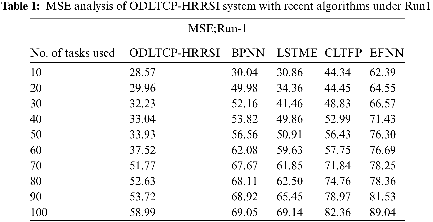
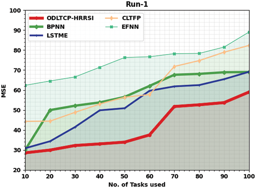
Figure 3: MSE analysis of ODLTCP-HRRSI system under Run1

Table 2 and Fig. 4 illustrate a detailed MSE analysis of the ODLTCP-HRRSI approach with existing models under run-2. The results denoted the ODLTCP-HRRSI algorithm has obtained minimal MSE values. For example, on 10 tasks, the ODLTCP-HRRSI methodology has reached the least MSE of 23.50, whereas the BPNN, LSTME, CLTFP, and EFNN methods have increased MSE of 30.65, 31.45, 49.40, and 62.06 correspondingly. Also, on 100 tasks, the ODLTCP-HRRSI methodology has reached least MSE of 55.46, whereas the BPNN, LSTME, CLTFP, and EFNN techniques have increased MSE of 68.99, 69.77, 79.97, and 89.99 correspondingly.

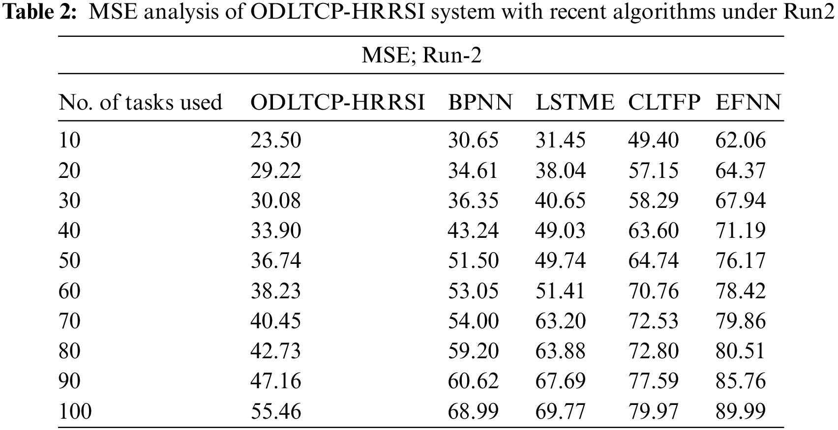
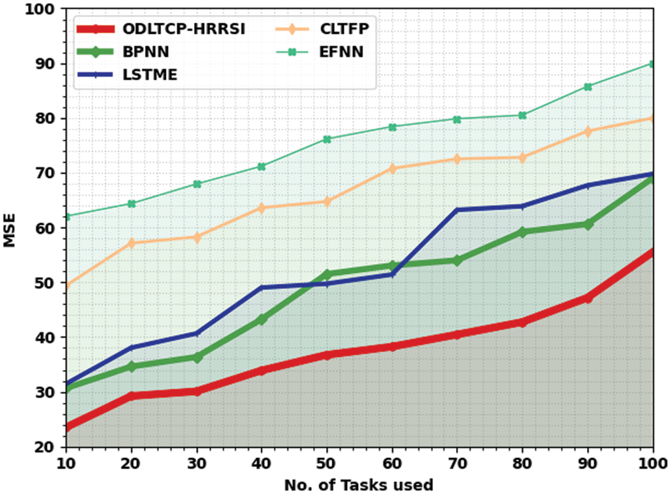
Figure 4: MSE analysis of ODLTCP-HRRSI system under Run2

Table 3 and Fig. 5 illustrate a brief MSE review of the ODLTCP-HRRSI technique with existing algorithms under run-3. The outcomes exemplified by the ODLTCP-HRRSI approach have gained minimal MSE values. For example, on 10 tasks, the ODLTCP-HRRSI algorithm has reached a minimal MSE of 21.28, whereas the BPNN, LSTME, CLTFP, and EFNN methods have obtained increased MSE of 30.11, 30.43, 41.22, and 60.12 correspondingly. In addition, on 100 tasks, the ODLTCP-HRRSI algorithm has reached least MSE of 52.71, whereas the BPNN, LSTME, CLTFP, and EFNN methods have gained increased MSE of 63.63, 75.14, 81.41, and 93.70 correspondingly.

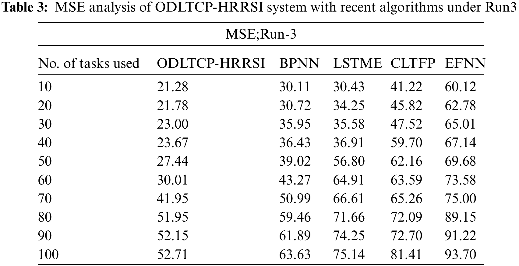
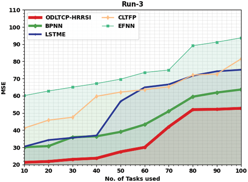
Figure 5: MSE analysis of ODLTCP-HRRSI system under Run3

Table 4 and Fig. 6 validate a brief MSE examination of the ODLTCP-HRRSI approach with existing models under run-4. The results denoted the ODLTCP-HRRSI approach has attained minimal MSE values. For example, on 10 tasks, the ODLTCP-HRRSI approach reached the least MSE of 21.26, whereas the BPNN, LSTME, CLTFP, and EFNN approaches have obtained increased MSE of 31.61, 30.36, 47.14, and 60.33 correspondingly. Also, on 100 tasks, the ODLTCP-HRRSI approach has achieved the least MSE of 57.93, whereas the BPNN, LSTME, CLTFP, and EFNN methods have increased MSE of 65.73, 74.66, 86.67, and 88.76 correspondingly.

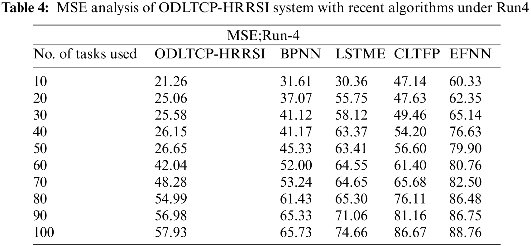
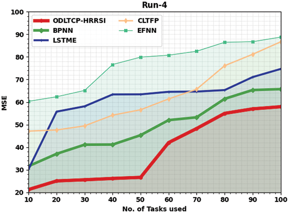
Figure 6: MSE analysis of ODLTCP-HRRSI system under Run4

Table 5 and Fig. 7 portray a comparative MSE review of the ODLTCP-HRRSI method with existing models under run-5. The results denoted the ODLTCP-HRRSI algorithm has attained minimal MSE values. For example, on 10 tasks, the ODLTCP-HRRSI approach has reached the least MSE of 22.85, whereas the BPNN, LSTME, CLTFP, and EFNN models have gained increased MSE of 32.69, 30.26, 41.62, and 61.28 correspondingly. Also, on 100 tasks, the ODLTCP-HRRSI technique has reached the least MSE of 54.16, whereas the BPNN, LSTME, CLTFP, and EFNN approaches have increased MSE of 65.11, 75.35, 87.73, and 86.47 correspondingly.

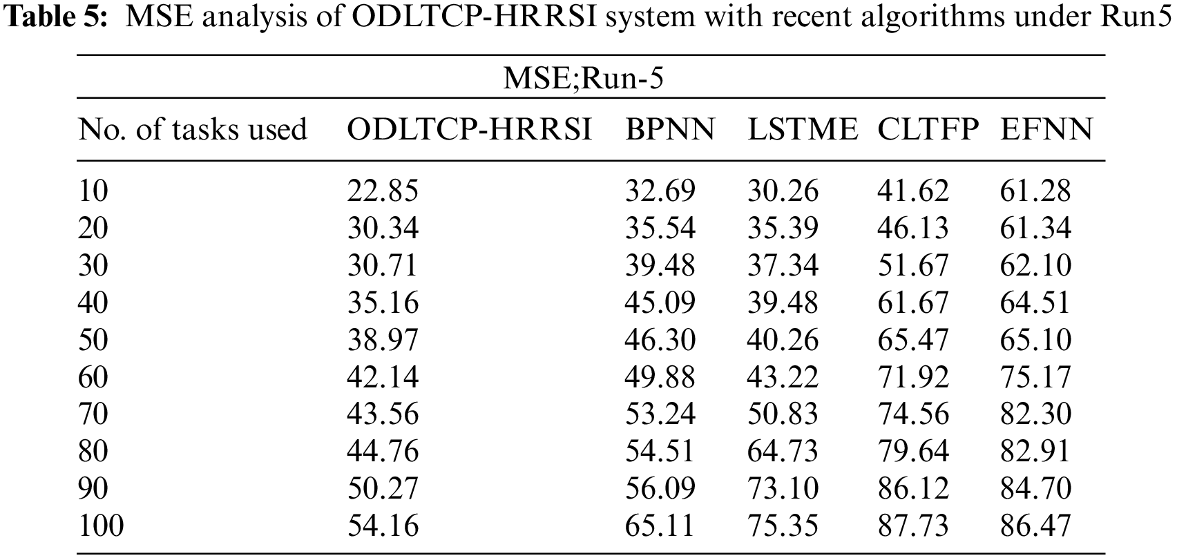
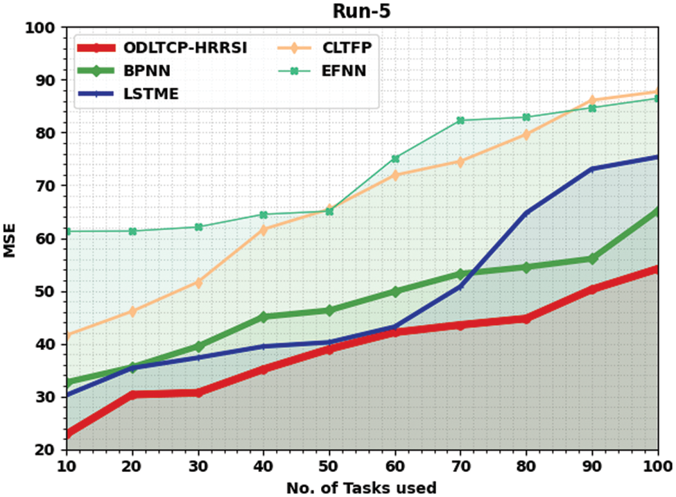
Figure 7: MSE analysis of ODLTCP-HRRSI system under Run5

The training time (TRT) study of the ODLTCP-HRRSI model and existing models are analyzed in Table 6 and Fig. 8. The experimental values indicated that the ODLTCP-HRRSI model had reached reduced values of TRT under all tasks. For instance, on 10 tasks, the ODLTCP-HRRSI model obtained a lower TRT of 13.80 ms, whereas the BPNN, LSTME, CLTFP, and EFNN models have reached increased TRT of 26.55 ms, 20.97 ms, 30.51 ms, and 50.80 ms respectively.

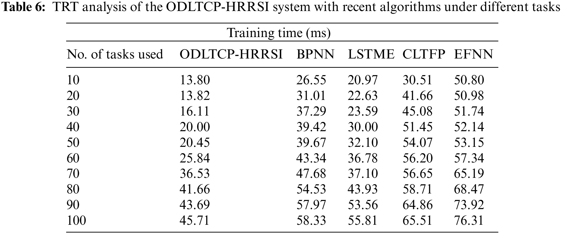
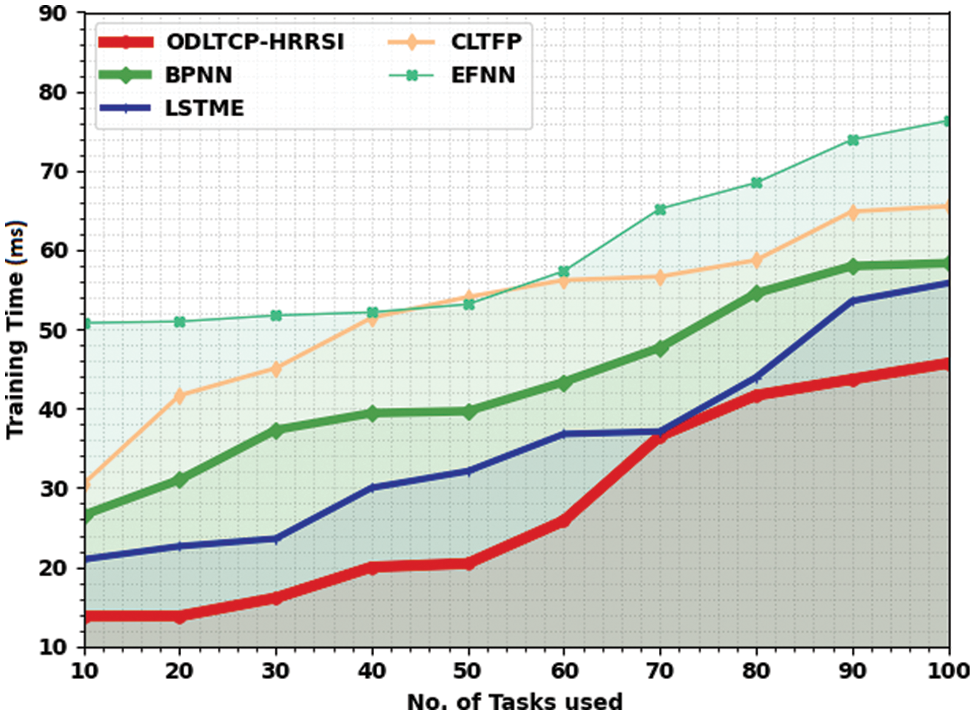
Figure 8: TRT analysis of the ODLTCP-HRRSI system under different tasks

On the other hand, on 50 tasks, the ODLTCP-HRRSI method has reached a lower TRT of 20.45 ms, whereas the BPNN, LSTME, CLTFP, and EFNN approaches have reached increased TRT of 39.67 ms, 32.10 ms, 54.07 ms, and 53.15 ms correspondingly. Last, on 100 tasks, the ODLTCP-HRRSI approach gained a lower TRT of 45.71 ms whereas the BPNN, LSTME, CLTFP, and EFNN algorithms have attained increased TRT of 58.33 ms, 55.81 ms, 65.51 ms, and 76.31 ms correspondingly.

A comparative accuy examination of the ODLTCP-HRRSI model with existing models is given in Table 7 and Fig. 9. The results demonstrated the enhanced outcomes of the ODLTCP-HRRSI model with higher accuy values. For instance, on 10 tasks, the ODLTCP-HRRSI model has offered an increased accuy of 97.20%, whereas the BPNN, LSTME, CLTFP, and EFNN models have attained reduced accuy of 95.25%, 95.87%, 92.59%, and 95.25% respectively. Meanwhile, on 50 tasks, the ODLTCP-HRRSI method has presented an increased accuy of 97.56%, whereas the BPNN, LSTME, CLTFP, and EFNN algorithms have reached reduced accuy of 95.98%, 96.16%, 93.14%, and 95.44% correspondingly. Eventually, on 100 tasks, the ODLTCP-HRRSI methodology has presented an increased accuy of 97.52%, whereas the BPNN, LSTME, CLTFP, and EFNN techniques have achieved reduced accuy of 94.39%, 95.57%, 91.91%, and 94.39% correspondingly.

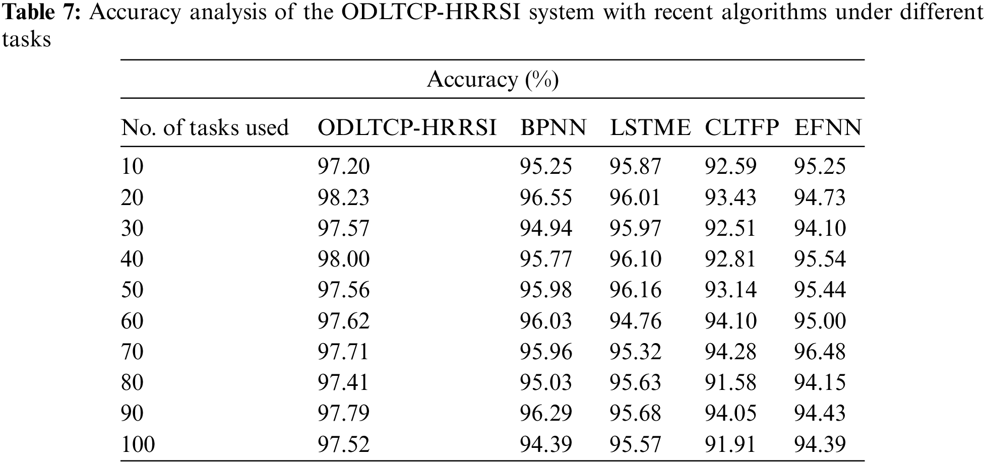
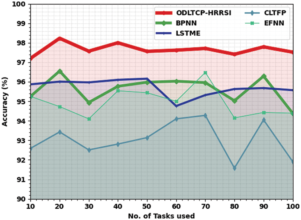
Figure 9: Accuracy analysis of the ODLTCP-HRRSI system under different tasks

The training accuracy (TRA) and validation accuracy (VLA) acquired by the ODLTCP-HRRSI methodology under the test database is exemplified in Fig. 10. The experimental result denoted the ODLTCP-HRRSI approach has accomplished maximal values of TRA and VLA. The VLA is greater than TRA.

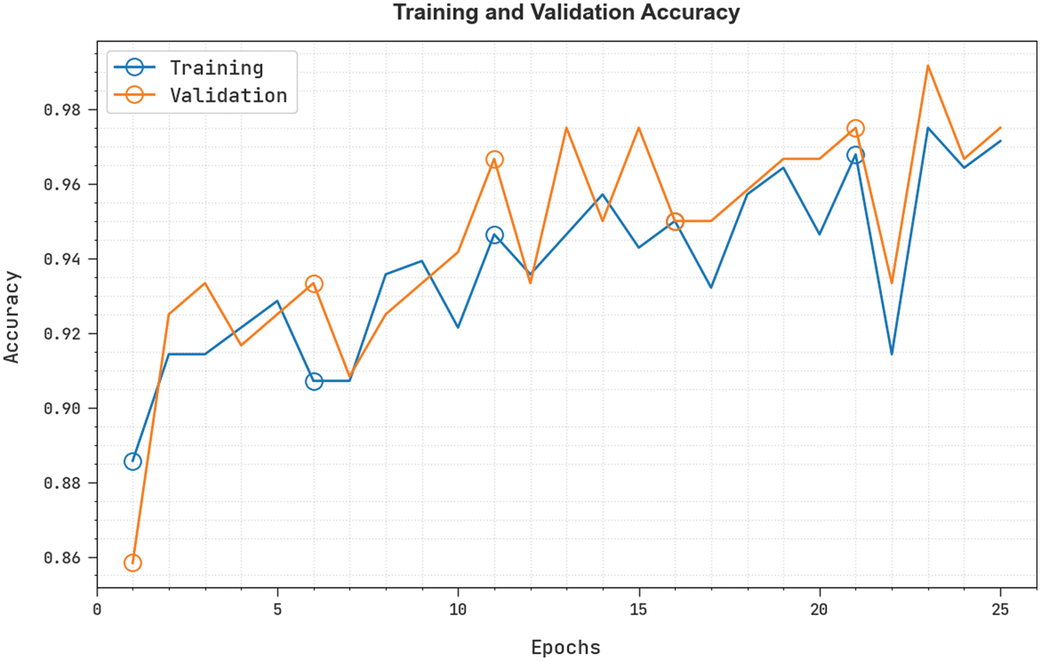
Figure 10: TRA and VLA analysis of the ODLTCP-HRRSI system

The training loss (TRL) and validation loss (VLL) reached by the ODLTCP-HRRSI technique under the test database are shown in Fig. 11. The experimental result designated the ODLTCP-HRRSI algorithm has achieved least values of TRL and VLL. Particularly, the VLL is lesser than TRL. Hence, the ODLTCP-HRRSI model is found to be effective over other models.

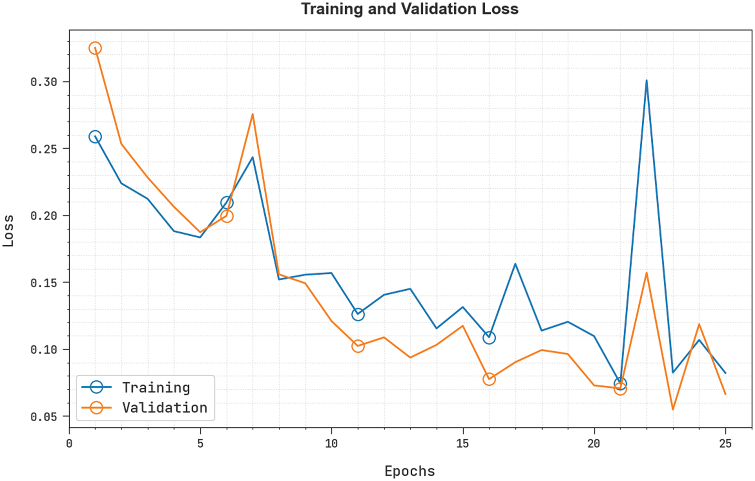
Figure 11: TRL and VLL analysis of the ODLTCP-HRRSI system

5  Conclusion

This article has developed a new ODLTCP-HRRSI technique to forecast critical traffic in smart cities. To attain this, the presented ODLTCP-HRRSI model performs two major processes. At the initial stage, the ODLTCP-HRRSI technique employed the CNN-AE model for productive and accurate traffic flow. Next, the hyperparameter adjustment of the CNN-AE model is performed via the BADSO algorithm. The experimental evaluation of the ODLTCP-HRRSI technique takes place, and the results are assessed under distinct aspects. The experimental outcomes demonstrate the enhanced performance of the ODLTCP-HRRSI technique over the recent state-of-the-art approaches. In the future, multiple DL-based fusion models can be derived to improve traffic prediction outcomes.

Funding Statement: The authors received no specific funding for this study.

Conflicts of Interest: The authors declare they have no conflicts of interest to report regarding the present study.

References

1. B. Alsolami, R. Mehmood and A. Albeshri, “Hybrid statistical and machine learning methods for road traffic prediction: A review and tutorial,” in Smart Infrastructure and Applications EAI/Springer Innovations in Communication and Computing book series, Cham: Springer, pp. 115–133, 2020. [Google Scholar]

2. S. Khanal, A. Klopfenstein, K. C. Kushal, V. Ramarao, J. Fulton et al., “Assessing the impact of agricultural field traffic on corn grain yield using remote sensing and machine learning,” Soil and Tillage Research, vol. 208, pp. 104880, 2021. [Google Scholar]

3. T. Jia and P. Yan, “Predicting citywide road traffic flow using deep spatiotemporal neural networks,” IEEE Transactions on Intelligent Transportation Systems, vol. 22, no. 5, pp. 3101–3111, 2020. [Google Scholar]

4. P. Cao, F. Dai, G. Liu, J. Yang and B. Huang, “A survey of traffic prediction based on deep neural network: Data, methods and challenges,” in Int. Conf. on Cloud Computing Lecture Notes of the Institute for Computer Sciences, Social Informatics and Telecommunications Engineering Book Series, Cham, Springer, vol. 430, pp. 17–29, 2022. [Google Scholar]

5. A. Wang, J. Xu, R. Tu, M. Saleh and M. Hatzopoulou, “Potential of machine learning for prediction of traffic related air pollution,” Transportation Research Part D: Transport and Environment, vol. 88, no. March, pp. 102599, 2020. [Google Scholar]

6. W. Jiang and L. Zhang, “Geospatial data to images: A deep-learning framework for traffic forecasting,” Tsinghua Science and Technology, vol. 24, no. 1, pp. 52–64, 2018. [Google Scholar]

7. Y. Chen, R. Qin, G. Zhang and H. Albanwan, “Spatial temporal analysis of traffic patterns during the COVID-19 epidemic by vehicle detection using planet remote-sensing satellite images,” Remote Sensing, vol. 13, no. 2, pp. 208, 2021. [Google Scholar]

8. A. Ganji, M. Zhang and M. Hatzopoulou, “Traffic volume prediction using aerial imagery and sparse data from road counts,” Transportation Research Part C: Emerging Technologies, vol. 141, pp. 103739, 2022. [Google Scholar]

9. Y. Zhang, X. Dong, L. Shang, D. Zhang and D. Wang, “A multi-modal graph neural network approach to traffic risk forecasting in smart urban sensing,” in 17th Annual IEEE Int. Conf. on Sensing, Communication, and Networking (SECON), Como, Italy, pp. 1–9, 2020. [Google Scholar]

10. S. He, M. A. Sadeghi, S. Chawla, M. Alizadeh, H. Balakrishnan et al., “Inferring high-resolution traffic accident risk maps based on satellite imagery and gps trajectories,” in Proc. of the IEEE/CVF Int. Conf. on Computer Vision, Montreal, QC, Canada, pp. 11977–11985, 2021. [Google Scholar]

11. G. Kothai, E. Poovammal, G. Dhiman, K. Ramana, A. Sharma et al., “A new hybrid deep learning algorithm for prediction of wide traffic congestion in smart cities,” Wireless Communications and Mobile Computing, vol. 2021, no. 8, pp. 1–13, 2021. https://doi.org/10.1155/2021/5583874 [Google Scholar] [CrossRef]

12. W. Wang, R. D. J. Samuel and C. H. Hsu, “Prediction architecture of deep learning assisted short long term neural network for advanced traffic critical prediction system using remote sensing data,” European Journal of Remote Sensing, vol. 54, no. sup2, pp. 65–76, 2021. [Google Scholar]

13. S. Patel, N. Ganatra and R. Patel, “Multi-level feature extraction for automated land cover classification using deep cnn with long short-term memory network,” in 6th Int. Conf. on Trends in Electronics and Informatics (ICOEI), Tirunelveli, India, pp. 1123–1128, 2022. [Google Scholar]

14. S. Byun, I. K. Shin, J. Moon, J. Kang and S. I. Choi, “Road traffic monitoring from UAV images using deep learning networks,” Remote Sensing, vol. 13, no. 20, pp. 4027, 2021. [Google Scholar]

15. F. Dai, P. Huang, X. Xu, L. Qi and M. R. Khosravi, “Spatio-temporal deep learning framework for traffic speed forecasting in IoT,” IEEE Internet of Things Magazine, vol. 3, no. 4, pp. 66–69, 2020. [Google Scholar]

16. A. A. Ahmed, B. Pradhan, S. Chakraborty, A. Alamri and C. W. Lee, “An optimized deep neural network approach for vehicular traffic noise trend modeling,” IEEE Access, vol. 9, pp. 107375–107386, 2021. [Google Scholar]

17. H. Yang, X. Zhang, Z. Li and J. Cui, “Region-level traffic prediction based on temporal multi-spatial dependence graph convolutional network from gps data,” Remote Sensing, vol. 14, no. 2, pp. 303, 2022. [Google Scholar]

18. K. Fukami, T. Nakamura and K. Fukagata, “Convolutional neural network based hierarchical autoencoder for non-linear mode decomposition of fluid field data,” Physics of Fluids, vol. 32, no. 9, pp. 095110, 2020. [Google Scholar]

19. Q. H. Feng, S. S. Li, X. M. Zhang, X. F. Gao and J. H. Ni, “Well production optimization using streamline features-based OF and Bayesian adaptive direct search algorithm,” Petroleum Science, vol. 19, no. 6, pp. 2879–2894, 2022. https://doi.org/10.1016/j.petsci.2022.06.016 [Google Scholar] [CrossRef]