GaitDONet: Gait Recognition Using Deep Features Optimization and Neural Network

1  Introduction

Gait refers to the movement and stability of the human body when walking straight, which is the plain movement style of the inferior limbs [1]. Human identification using biometric techniques has become a major issue in recent years, and these biometric techniques are used to solve the problem of human gait recognition from a distance [2]. Fingerprint, handwriting, ear, iris, and face detection are all human identification techniques that are used to identify humans based on their unique individual features. Every person on the planet has unique iris patterns and fingerprints that are used to identify them [3]. The primary application of gait recognition is in security systems. In today’s technological era, a creative and forward-thinking biometric application is required, and the gait is an ideal methodology for recognizing people. Human gait recognition has the advantage over other techniques in that it produces positive results while avoiding identification from low-resolution videos [4]. Human gait recognition (HGR) is a critical biometric technique because each individual has distinct characteristics such as walking style, clothing variations, carrying condition, and angle variations [5].

Human gait is increasingly inspiring researchers as a biometric technique. It is more important than fingerprint and face recognition technologies [5]. The HGR has developed an active study zone and significant attention in the field of Computer Vision (CV) [6,7]. Every human has common and familiar gait patterns. HGR is a complicated method because it relates to examination points. HGR has two approaches: model-based approach and model-free approach [4,8]. The model-based approach directs human movement based on prior knowledge, whereas the model-free approach creates human body sketches [9,10]. To investigate human activities based on upper/lower body parts and joint movements, a model-based approach is used. The model-free approach, on the other hand, requires less computational time and is easier to implement. Numerous computer-based techniques have been introduced into the literature by CV researchers [11]. The methods presented are based on traditional and deep learning techniques. Traditional techniques involve a number of steps, including data preprocessing [12], region of interest (ROI) detection, feature extraction, and classification [13]. The extraction of the ROI is a critical step in traditional gait recognition techniques. The main goal of this step is to extract features from only the most important region [14]. The following step is feature reduction, which has the primary goal of removing redundant features. Principle component analysis (PCA), entropy, and other techniques are used for feature reduction.

Many deep learning-based HGR methods are discussed in the literature. Convolutional neural network (CNN) is a deep learning model used for a wide range of tasks such as object recognition [15], action recognition [16], gait recognition, medical imaging [17], and many more [18,19]. A convolutional layer, an activation layer, a feature extraction layer, and a classification layer comprise the CNN model [20]. Bari et al. [21] presented a deep learning based framework for HGR. They used several deep learning methods and at the end performed features fusion and features selection. Khan et al. [2] presented a framework with four major steps. In the first step, the dataset is normalized from a video frame. In the second step, transfer learning (TL) is used to fine-tune and train pre-trained InceptionV3 and ResNet101 deep models. In the following step, features are extracted and improved ant colony optimization is performed to select the best features. The experiment was carried out on the CASIA B dataset and yielded notable accuracy. Wang et al. [11] introduced an convolutional longer shortest memory (Conv-LSTM) architecture for human gait recognition. In this method, gait energy images (GEI) is presented frame by frame, and then volume is expended to reduce gait cycle constraints. For the cross covariance analysis, only one subject is used in the experimental process. HGR is completed in the final step using the Conv-LSTM model. The CASIA B and large-scale gait (OU-ISIR) datasets were used for validation, with accuracy rates of 93% and 95%, respectively.

Arshad et al. [1] presented a framework for HGR based on feature fusion and optimal feature selection. For feature extraction, two pre-trained deep learning models named Alexnet and very deep network (VGG19) are used. On both deep feature vectors, a new approach called entropy controlled skewness (FEcS) is used to select the best features. The experiments were carried out on several datasets and yielded accuracy rates of 99.8%, 99.7%, 93.3%, and 92.2%. The disadvantage of this method is that it ignores a few important features that could improve the accuracy of the CASIA B dataset. Mehmood et al. [8] presented a deep learning-based HGR system. The presented method consists of four steps: video frame preprocessing, deep learning feature extraction, feature selection, and classification. The selection of best features using the firefly algorithm was the work’s strength. The presented method was tested on the CASIA B dataset and achieved accuracy of 94.3%, 93.8%, and 94.7%, respectively. Anusha et al. [22] extracted texture, spatial, and gradient information from video frames for HGR, which is known as low level features. The experiments were carried out on five datasets and yielded improved accuracy. Sharif et al. [23] extract features and regions of interest (ROI). They also performed multilevel feature fusion to gain a better understanding of human gait. Wu et al. [24] presented a graph-based HGR approach. They used Spiderweb graph connections to connect angles in this approach. The experiments were carried out on the sdu gait dataset, the Multi-View Large Population Dataset (OU-MVLP) dataset, and the CASIA B dataset, with accuracies of 98.54%, 96.91%, and 98.77%, respectively. In summary, the methods described above aimed to improve the accuracy of HGR through the use of multiple datasets. However, there is a discrepancy in the accuracy of the CASIA B dataset, and these methods did not take the entire dataset into account during the experimental process. They also used feature selection techniques but didn’t mention the computational time based comparison. In this paper, we proposed a new architecture based on the fusion of deep learning models, information fusion, and an improved manta ray foraging optimization (MRFO) algorithm.

2  Proposed Methodology

The proposed human gait recognition architecture is depicted in Fig. 1. This diagram depicts how the original video frames are processed and fine-tuned deep learning models such as Squeezenet and Efficientnet are trained for all 11 selected angles. Deep transfer learning was used to train both fine-tuned models on gait datasets, resulting in two new targeted models used for feature engineering. Using multi-set canonical correlation analysis, features are extracted from the deep layer of both fine-tuned models and fused into a single vector (MCCA). The fused feature vector is then optimized with an improved manta ray foraging optimization algorithm to select the best features, which are then classified with a narrow neural network classifier. Each substep in this diagram is described in detail below.

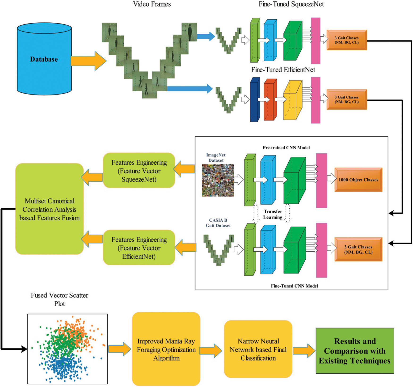
Figure 1: Proposed architecture of human gait recognition using deep learning and features optimization

2.1 CASIA B Dataset

In this work, we utilized CASIA B dataset for the experimental process. This dataset contains 124 subjects and for each subject, 10 samples are captured from 11 viewing angles such as 0, 18, 36, 54, 72, 90, 108, 126, 144, 162 and 180. Each subject performed these 11 angles for three different scenarios such as normal walk (6 videos), walk with carrying a bag (2 videos), and walk with wearing a coat (2 videos). Each video is recorded under the image resolution of 352 × 240 × 3 (rgb) and with 25 fps [25]. A few sample images are shown in Fig. 2.

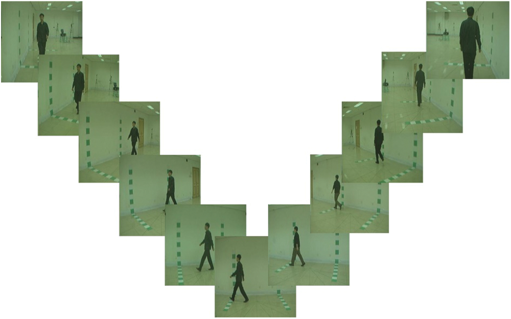
Figure 2: Sample frames of CASIA B dataset for all 11 viewing angles

2.2 Convolutional Neural Network (CNN)

Convolutional neural network (CNN) is a powerful type of artificial neural network (ANN) that can handle large datasets with improved performance. Thus, for accurate pattern recognition tasks, networks encode image features better than ANN. A CNN network is made up of several layers, including an input layer, a convolutional layer, a pooling layer, a batch normalization layer, a fully connected layer, and a softmax classification layer.

The convolutional layer’s primary function is to learn how to represent the input based on its features. Several different feature maps can be computed in the convolutional layer by using different convolution kernels. Every previous layer’s neurons are precisely connected to each of the current feature layer’s corresponding neurons. According to the previous neuron, this is known as a neuron’s receptive field. It is worth noting that every single feature map is generated by sharing the kernel with all of the input data’s special locations. We can calculate the value of the feature at (p,q) location in the mth feature map of the nth layer.

ap,q,mn=wmnTxp,qn+bmn(1)

In the above equation wmn and bmn these are the weight vector and the bias term of the mth feature map of the nth layer respectively. xp,qn is the input area at the center of the (p,q) location of the nth layer. It is worth noting that kernel wmn is shared, which produces the a:,:,mn feature map. There are numerous benefits to this weight-sharing technique, for example, it makes the training of the model much easier and can reduce its complexity. The nonlinearities to CNN is presented by the activation function, the nonlinear features are identified by the multi-layer networks. Here the i(.) represent the nonlinear activation function, hence the activation value ip,q,mn of the convolutional feature ap,q,mn can be calculated by:

ip,q,mn=i(ap,q,mn)(2)

Generally tanh and rectified layer unit (ReLU) are the sigmoid activation functions. We can reduce the resolution of the feature maps by using the pooling layers in order to achieve shift-invariance. In the between the two convolutional layers the pooling layer is placed. Every single of a pooling layer is linked to its matching feature map of the previous convolutional layer. The pool(⋅), is representing the pool fuction and ip,q,mn is representing the each feature map.

Kp,q,mn=pool(ig,h,mn),∀(g . h)∈Npq(3)

In the above equation Npq is the local neighborhood around (p,q) location. In order for the pooling operation to work, generally max pooling and [26] average pooling are used. Fig. 2b demonstrations in the 1st convolutional layer the edges and curves that are consider as low-level features and these are detected through the kernels, while more abstract features are detected through the kernels in higher layers. Some convolutional and pooling layers are used increasingly for extract of the higher-level features.

After the convolutional and pooling layers for performing the high-level reasoning one or more FC-layer can be added. In order to generate global semantic information, they connect all neurons of the current layer with the corresponding neurons of the previous layer [27]. The last layer is the softmax layer which is the output layer, used for classification. Support vector machine (SVM) is also used for classification, combined with CNN features [28]. Let µ represent the CNN parameters. We can minimize the loss function in order to obtain the optimum parameters [29,30]. Let’s assume that there are M preferred input-output relations.

We have M preferred input-output relations. {(i(n),j(n));n∈[1,…,M]}, where i(n) is the nth input data and j(n) is its corresponding target data. Let the output of the CNN is O(n). The loss of CNN can be calculate as:

L=1M∑n=1Ml(µ;j(n),O(n))(4)

Global Optimization can be obtained by training CNN. The best matching set of parameters can be found by minimizing the loss function. A usual explanation for the optimizing the CNN network is the Stochastic Gradient.

2.3 Deep Learning Models for Features Extraction

SqueezeNet: The SqueezeNet is the convolution network which gives the better performance than the AlexNet [31,32]. There are fifteen layer on which SqueezeNet based, these layers consist of; the convolution layers are two, the max pooling layers are three, fire layers are eight, the global average pooling is one, and the one softmax layer. Here, K × K represents the field size of the filter; the length of the feature map is 1 and the size of the stride s, respectively. The dimensions and input size of the SqueezeNet is 227 × 227 with rgb channels. The convolution layer is used to generalized the input images, after that the max pooling is applied. In the input volume the convolution layer convolutes between the weights and small regions, with the kernels of 3 × 3. The positive part of its argument every convolution layer performed activation function by element wise. The fire layers, which constructed of squeeze and expansion phases and utilized by the SqueezeNet.

EfficientNetB0: In the baseline network the layer operators does not change by model scaling, it is critical of having good baseline network [33]. Convolutional network is used to evaluate the scaling methods, A new mobile size baseline, called EfficientNet is developed for the better demonstration and effective scaling methods. The EfficientNet is inspired by [34] in this paper author develop a baseline by the leveraging a multi-objective neural architecture search that optimizes both accuracy and floating point operations per second (FLOPS) [34].

Fine-Tuning of Pre-Trained CNN Models: In the fine-tuning process, the last fully connected and successive connected layers have been removed. After that, new fully connected layer and connected classification layers have been added and assign weights. The deep transfer learning process is employed as a learning of both fine-tuned models from the scratch, as illustrated in Fig. 3. Mathematically, the definition of deep transfer learning is defined as follows:

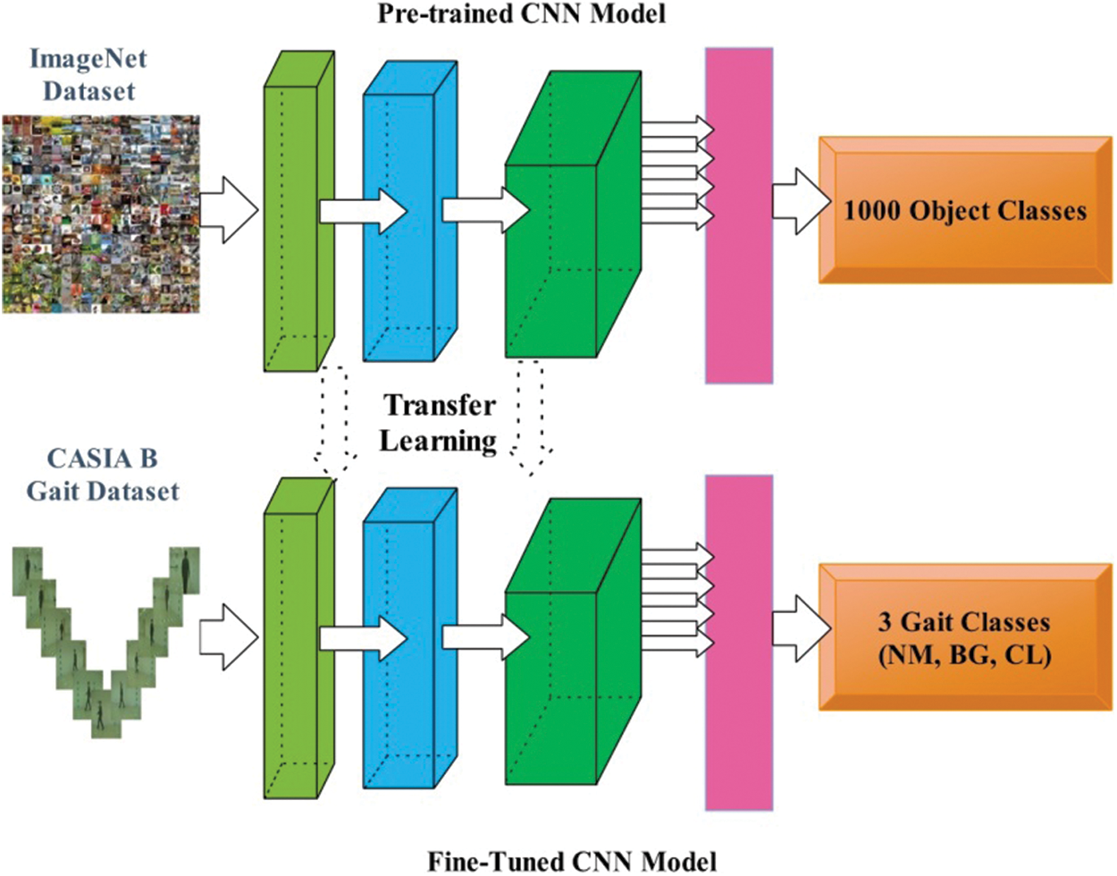
Figure 3: Deep transfer learning based training of pre-trained CNN modes for human gait recognition

Given a transfer learning task {Φs,ϖs,Φt,ϖt,fτ(.)}. It represent the deep transfer learning task where fτ(.) is a non-linear function that reflected a deep neural network.

For the training process, several hyper parameters have been assigned such as learning rate of gradient descent is 0.00001, momentum is 0.6, number of epochs are 100, batch size is 32, activation function is sigmoid, dropout rate is 0.5, and loss function for features extraction is cross entropy.

Deep Features Extraction: Consider, we have two new trained fine-tuned deep models are Δ1 and Δ2. The sigmoid function is utilized as an activation function for features extraction; hence deep features from global average pooling layer is computed for both models as follows:

V1=ξ(Δ1,Lgap)(5)

V2=ξ(Δ2,Lgap)(6)

The dimension of extracted deep features for both models is N×1280 and N×512, respectively. The obtained feature vectors are fused in single matrix using a modified multi-set canonical correlation analysis.

2.4 Modified MCCA Based Features Fusion

Assume that modality datasets P {X(r)=[x1(r),x2(r),…,xN(r)]∈Yvr×N}r=1P and this represent the sample of mth and the modality of rth dataset Xr. The multi-modal feature fusion method belongs to MCCA, and its goal is finding the association projection direction Φ(r)∈Yvr×1 association to X(r)(p=1,2,…,P). The optimization function MCCA’s is shown below:

max{Φr}r−1PΣr=1PΣs=1PΦ(r)LC(rs)Φ(s)Σr=1PΦ(r)LC(rr)Φ(r)(7)

Here C(rs)=1NΣm=1N(xm(r)−x−(r))(xm(s)−x−(s))L present covariance matrix for the X(r) and X(s), also the C(rr)=1NΣm=1N(xm(r)−x−(r))(xm(s)−x−(s))L, this present the variance matrix X(r)(p=1,2,…,P). In the above equation, the optimization function is transformed to the problem of constraint-based optimization.

max{Φr}r−1PΣr=1PΣs=1PΦ(r)LC(rs)Φ(s)(8)

s.t.Σr=1PΦ(r)LC(rr)Φ(r)=1(9)

In [28], Φ(r)LC(rr)Φ(r) these are the constrains between the modal and correlation features Φ(r)LX(r), Φ(s)LX(s) and Φ(r)LC(rr)Φ(r). The correlation features Φ(r)LX(r) can reveal by global scatter. The final features are fused in the descending order using the following equation:

Fd(i)={DS(Φ>μ)}(10)

The fused vector contains some irrelevant information that further optimized using improved Manta Ray Foraging Algorithm (IMRF).

2.5 IMRF Based Features Selection

Features selection is an important research topic now a days for several application but especially biometric. In this work, our main purpose is to propose an improved method for best feature selection from the input feature vector. The aim of this method is to improve the accuracy and reduce the computational time. We proposed an improved Manta Ray Foraging (IMRF) optimization algorithm for the best feature selection. The original Manta Ray Foraging Algorithm (MRFO) is inspired through three different foraging behaviors that includes cyclone foraging, chain foraging, and somersault foraging.

In MRF optimization, the manta rays judge the location or position of the plankton and then swim toward plankton. The position is better if concentration of the plankton in the position is high, while the best solution is unknown. The plankton is approaches and eaten by the manta rays, with higher concentration of that MRFO assume for the best solution. Manta rays from the foraging chain by line up by head-to-tail. In their movement, move is not towards the food only but toward also the one who is present in front of them. It happens in all the iterations and every solution is updated by the individual in front of it and best solution found so far. Mathematically, the chain foraging is defined as follows:

wja(s+1)={wja(s)+c . (wba(s)−wja(s))+β . (wba(s)−wja(s))j=1wja(s)+c . (wj−1a(s)−wja(s))+β . (wba(s)−wja(s))j=2,…,N(11)

β=2 . c . |log(c)|(12)

Here, wja(s) represent about the location of jth individuals when the time s in ath dimension, c represent the random vector whose range is within [0,1], and Plankton with higher concentration are wba(s). The updated position of each individual (jth) is described by the position wj−1(s) of the current individual (j−1)th and the position of food is wb(s).

Cyclone Foraging: When a spot of plankton recognized in deep water by manta rays of school, and they forms a long foraging chain and start swimming toward the food in the form of spiral. Whale optimization (WOA) found this similar spiral foraging strategy [35]. Although for strategy of cyclone foraging of the manta ray swarms, they are moves toward the food spirally, the manta rays are always swimming towards those who are in front of it. Foraging is performed by developing a spiral by manta rays. The movement of every individual towards the food along a spiral path but not only follows the one in front of it. In Eq. (13), the behavior of manta ray of spiral movement is defined as follows:

{Mj(s+1)=Mb+c . (Mj−1(s)−Mj(s))+fpd . cos⁡(2πd). (Mb−Mj(s))Nj(s+1)=Nb+c . (Nj−1(s)−Nj(s))+fpd . sin⁡(2πd). (Nb−Nj(s))(13)

where w is a random number between [0, 1]. The model of cyclone foraging is mathematically defined as follows:

wja(s+1)={wba+c . (wba(s)−wja(s))+α . (wba(s)−wja(s))j=1wba+c . (wj−1a(s)−wja(s))+α . (wba(s)−wja(s))j=2,…,N(14)

α=2fc1Z−z+1Z . sin⁡(2πc1)(15)

Here the coefficient of weight is α, maximum number of the iterations are represented by s, and the c1 represent random numbers between [0,1]. Every individual from the reference position performed random search to the food. Eq. (16) shows the mathematical model for the achievement of wide global search.

wra=Rpa+c . (Vpa−Rpa)(16)

wja(s+1)={wba+c . (wba(s)−wja(s))+α . (wra−wja(s))j=1wra+c . (wj−1a(s)−wja(s))+α . (wra−wja(s))j=2,…,N(17)

where w,a,r are the produced randomly position in the search space. The lower and upper limits of the a are Rpa and Vpa, respectively.

Somersault Foraging: In somersault behavior, the pivot is viewed as a position of the food. They are swimming to the new position based on pivot. When the best position found, then they update their positions as follows:

wja(s+1)=wja(s)+W . (c2 . wba−c3 . wja(s))(18)

Here, W is the somersault factor and initialized as 2, c2 and c3 are consist of two random numbers between [0,1]. In the above equation, this is feasible for everyone to move toward some position.The randomly distribute sampled points examined this locations and their balanced situations around the wb, and the distance of sample points is reduce. Like other metaheuristic optimization methods, In the MRF it is started from generating population randomly in the problem domain. At every repetition, the position is updated by every individual updated the with respect to front and reference position. The worth of s/Z diminishes from 1/Z to 1, performed exploratory and exploitative search.

We improved this algorithm output based on opposition based learning. According to this, each individual is updated as: (wj−a+ > wj−1−a+). In the opposite when w, (wj−a+ < wj−1−a+), its means that for the current population only the best individuals are consider for the further iterations, and the remaining population is removed. Based on the following formulation the effective solution is generated:

wj−a=wjmax+wjmin−wja(19)

where, wj−a denotes the opposing location for the wja, wjmax, and wjmin. These are signifying minimum and maximum constraints. The size is transformed by the primary individual:

wja(s)=10×N(20)

Here N shows the number of parameters. The size of the updated individuals for the further iterations is got from the following formulation:

wj−a+=round(wja×(1+&))(21)

The final selected features wj−a+ of dimensional N×726 are finally passed to machine learning classifiers for classification.

3  Experimental Results and Analysis

The experimental results of proposed method are discussed under this section.

3.1 Experimental Setup

The results of proposed HGR architecture are presented in this section in terms of numerical values and graphs. The proposed architecture is tested on CASIA B dataset. The detail of dataset is given under Section 4.1. In this work, we utilized 50% video frames for the training purpose and rest of the 50% for testing the proposed architecture. All results are computed using 10-Fold cross validation. The recognition accuracy is computed for each angle of CASIA B datasets (11 angles) and also finds the mean accuracy. As mentioned in Section 2.1, three different angles have been involved for each angle; therefore, the separate accuracy of each angle is also computed. Narrow neural network is selected for the classification purpose and compared the accuracy with few other well-known methods such as extreme learning machine, Bi-Layered neural network, Tri-Layered neural network, and multiclass support vector machine (SVM). The entire proposed architecture is tested on MATLAB 2021b using personal computer with 16 GB of RAM and 8 GB graphics card.

3.2 Results

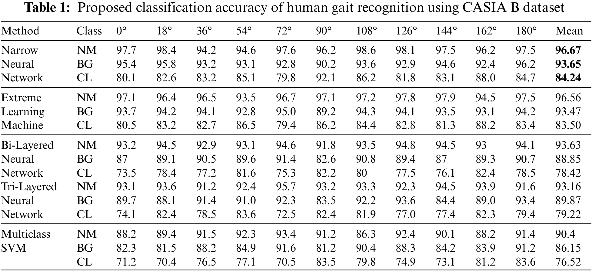
The proposed architecture results are presented in Table 1. In this table, the results of several classifiers are given for all 11 angles. For each angle, accuracy is computed for each class, separately. Narrow neural network attained average accuracy of 96.67%, 93.65%, and 84.24%, respectively for normal walk (NM), walk with carrying a bag (BG), and walk with wearing a coat (CL). The second selected classifier is extreme learning machine (ELM) and attained average accuracy of 96.56%, 93.47%, and 83.50%, respectively. The third selected classifier is Bi-Layered Neural Network and attained accuracy of 93.63%, 88.85%, and 78.42%, respectively. The fourth selected classifier is Tri-Layered Neural Network and attained accuracy of 93.16%, 89.87%, and 79.22%, respectively. The fifth selected classifier is multiclass SVM and attained accuracy of 90.4%, 86.15%, and 76.52%, respectively. Based on these results, it is observed that the overall accuracy of proposed gait recognition architecture is better for Narrow Neural Network, The values given in Table 1 also presents that the accuracy of each class for all 11 angles is better for this classifier.

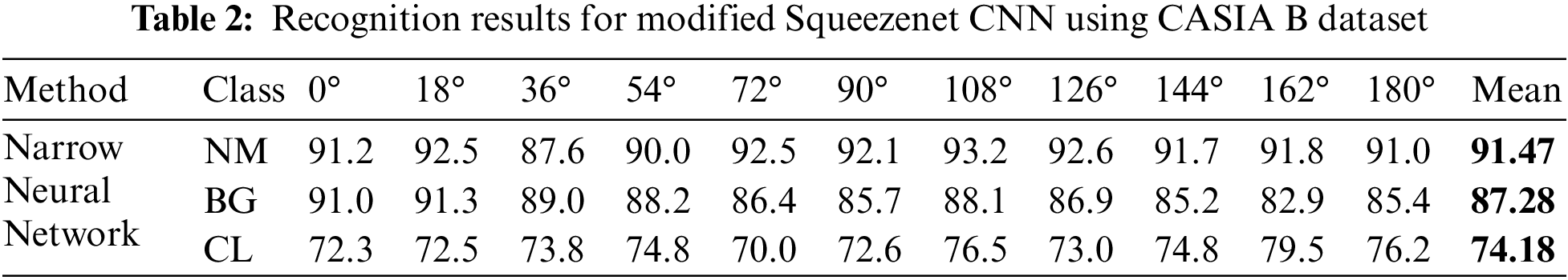
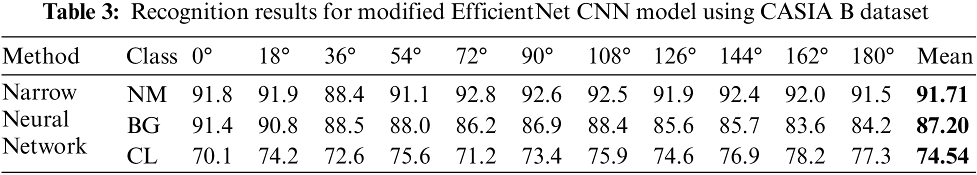
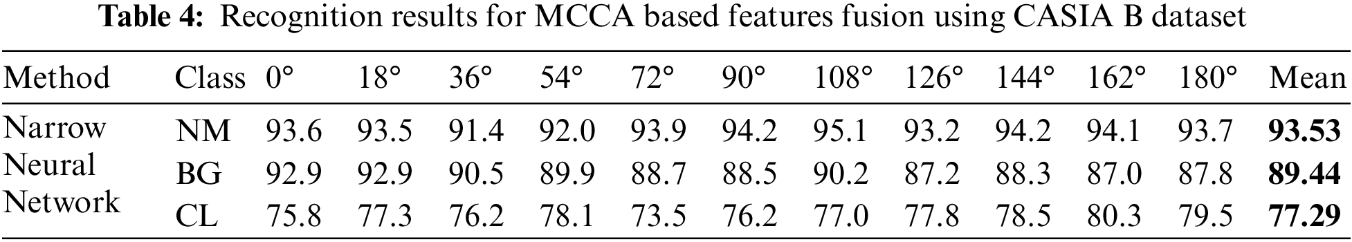
The proposed architecture accuracy is compared with individual steps such as modified Squeezenet CNN, modified EfficientNet, and MCCA based fusion. Table 2 presents the accuracy of Narrow Neural Network (NNN) for Squeezenet and attained an average accuracy of 91.47%, 87.28%, and 74.18%, respectively. Table 3 presents the accuracy of NNN for Efficientnet and attained an average accuracy of 91.71%, 87.20%, and 74.54%, respectively. This table shows that the performance of Efficientnet is better than the SqueezeNet. After the fusion process, accuracy is significantly improved and average accuracy is reached to 93.53%, 89.44%, and 77.29%, respectively, as presented in Table 4.

Moreover, the proposed feature selection algorithm performance is also analyzed based on different selection parameter value such as T = 0.3, T = 0.4, T = 0.5, T = 0.6, and T = mean value. The performance of each one is presented in Fig. 4. In this figure, it is shown that the accuracy of selection algorithm with T = 0.3 is 91.56%, 89.04%, and 78.65%, respectively. For T = 0.4, the attained accuracy is 92.5%, 90.68%, and 81.36%, respectively. This shows that the accuracy is improved after the change of T = 0.4. Similarly, the accuracy for T = 0.5 is 93.56%, 91.46%, and 82.04%, respectively. For T = 0.6, the obtained accuracy is 92.52%, 90.04%, and 80.14%, respectively. The increase in threshold value indicated that the accuracy is little reduced than the previous values. For T = mean value, the accuracy is little improved of 92.58%, 91.5%, and 82.36%, respectively. The proposed architecture obtained the improved accuracy than all values and obtained an accuracy of 96.67%, 93.65%, and 84.24%, respectively.

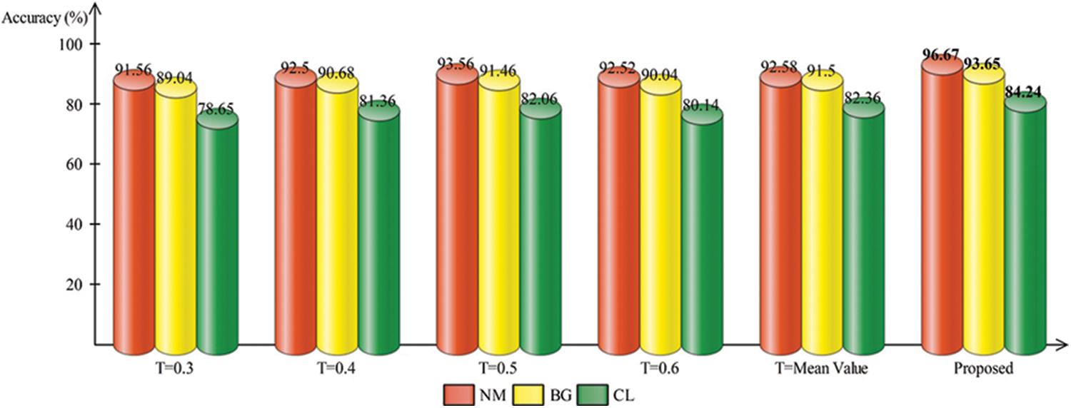
Figure 4: Comparison of different threshold values for features selection with proposed framework

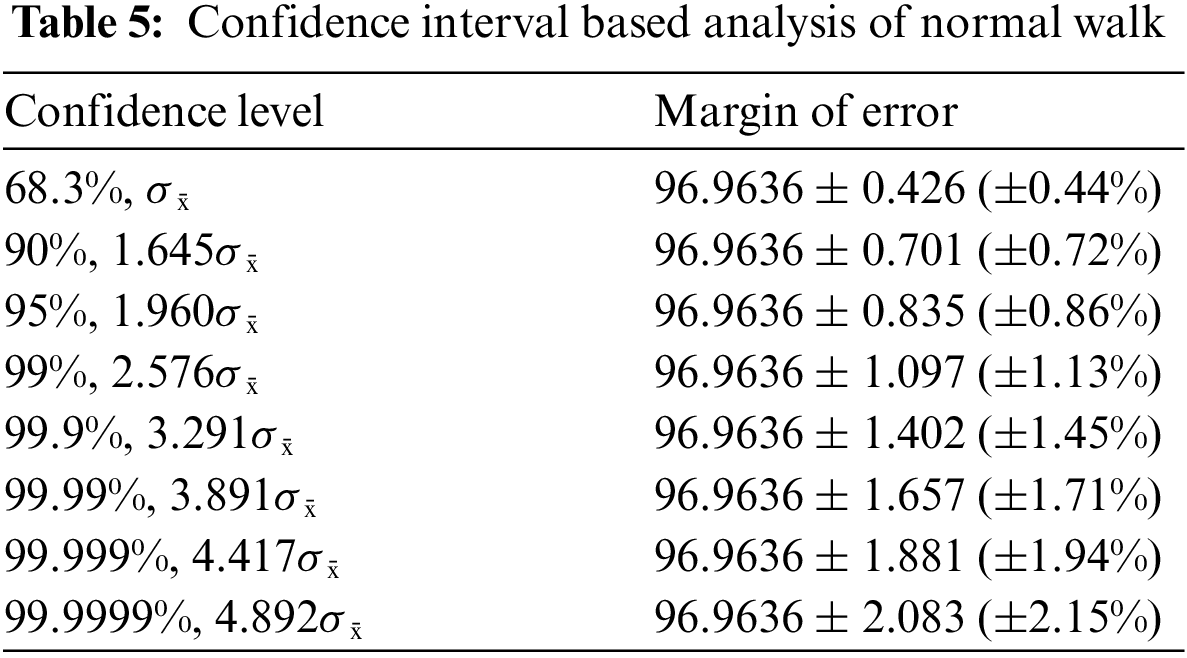
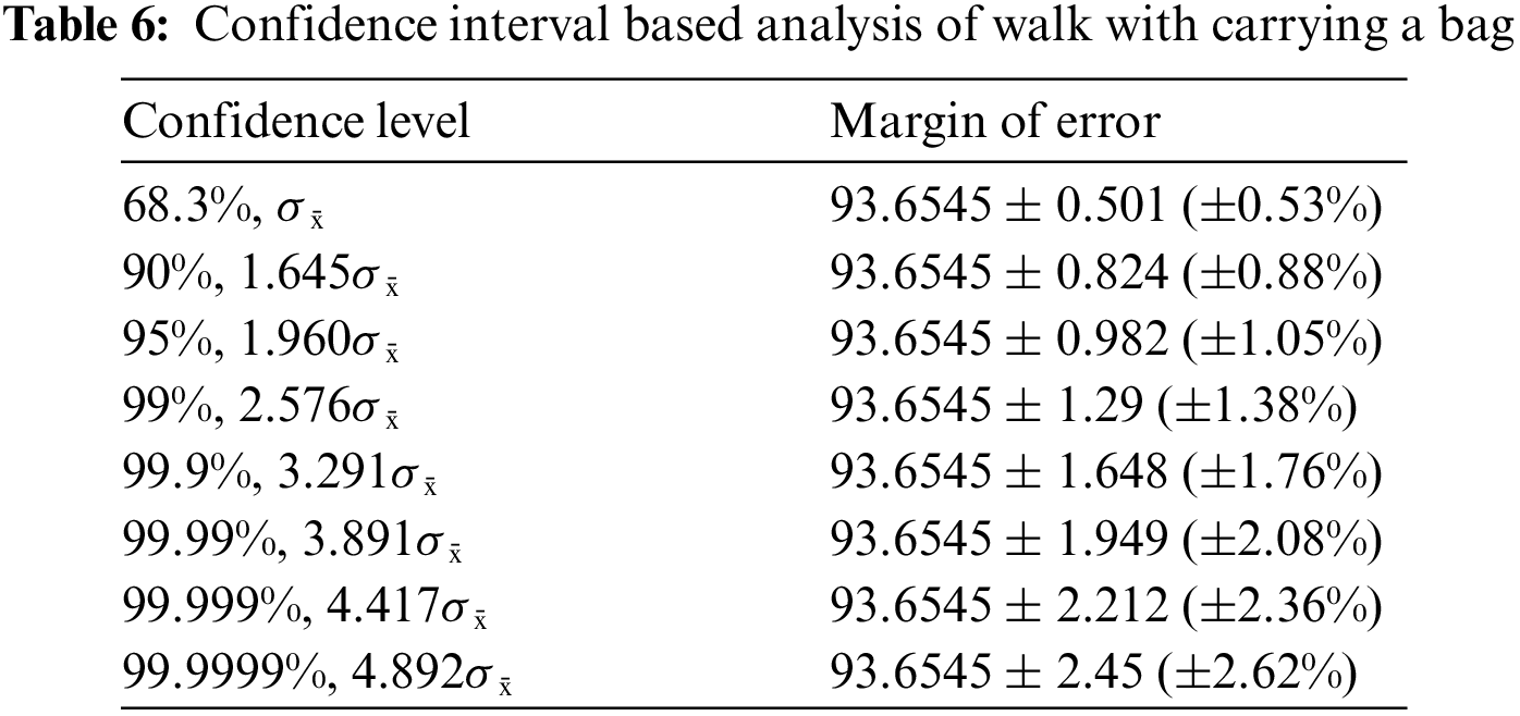
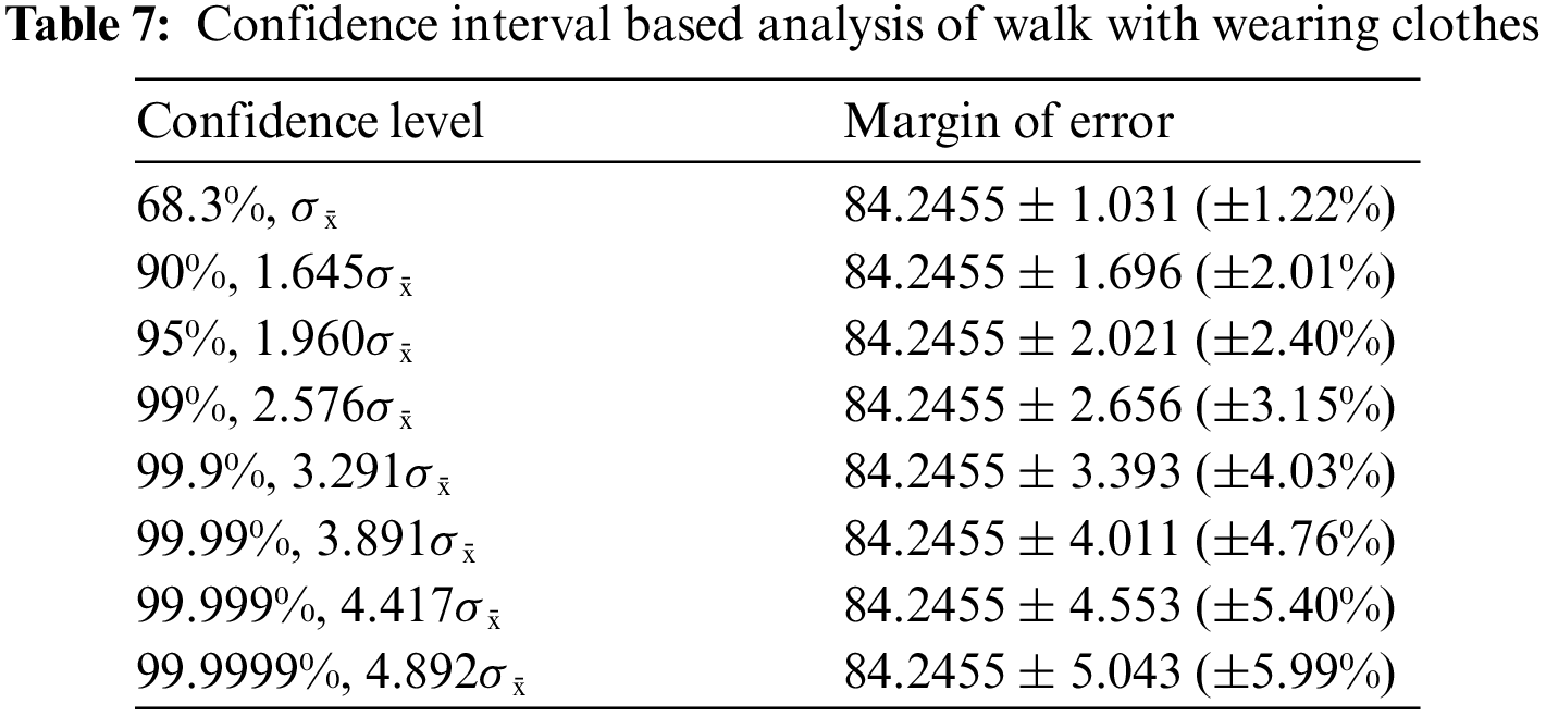
3.3 Confidence Interval Based Analysis and Comparison

A confidence interval (CI) based analysis is also conducted of proposed architecture using values of all 11 angles (given in Tables 5–7). Table 5 presents the CI based analysis of normal walk. In this table, the confidence level is defined and for each level, margin of error of (MoE) is computed. In this table for confidence level 95%, 1.960σ̄, the obtained MoE is 96.9636 ± 0.835 (±0.86%). For 90%, 1.645σ̄, the MoE is 96.9636 ± 0.701 (±0.72%). This shows that the accuracy is consistent and reliable of proposed architecture for normal walk.

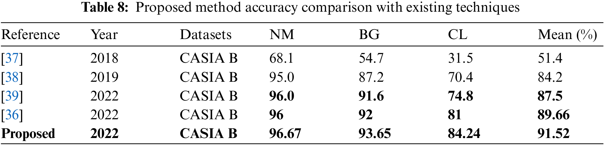
Time based comparison is also conducted, as illustrated in Fig. 5. In this figure, it is shown that the modified Squeezenet deep model consumes less time than the modified efficientnet. Later on, the fusion process consumes higher time than the previous two steps, but based on the above tables, it is also noted that the accuracy is improved for this step (fusion). Finally, the proposed selection step is also employed and it is shown that the time is significantly reduced. At the end, a brief comparison with some recent techniques is also conducted (Table 8). From this table, it is shown that the proposed method achieved improved accuracy on selected dataset for all three angles. The average accuracy of proposed method is 91.52 (sec), which is previously 89.66 by Li et al. [36].

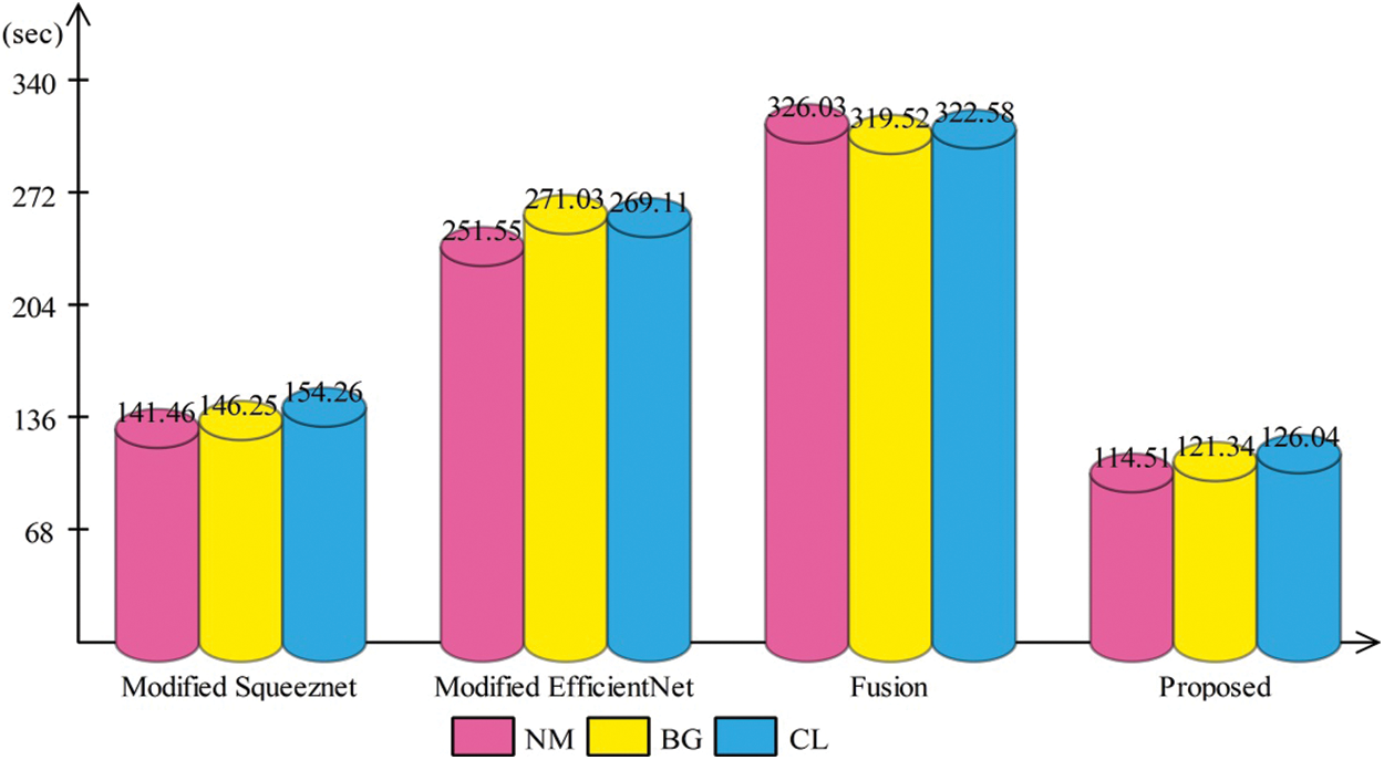
Figure 5: Time based comparison of proposed approach with middle steps

4  Conclusion

This work proposes a fusion of the deep best-selected features method for human gait recognition. The recent studies focused on feature extraction and then performed reduction, further utilized for final classification. Moreover, they also concentrated on a few angles instead of all 11 angles. In this work, we performed improved MCCA (IMCCA) based deep features fusion, further refined using an improved optimization technique. In the classification phase, the Narrow Neural Network gives better recognition accuracy. The experimental process was conducted on all 11 angles of the CASIA B dataset and achieved an average accuracy of 91.52%. As per our knowledge, it is the first gait recognition framework in which improved MCCA is applied for deep features fusion. The proposed method results are also compared with some recent techniques and show an improvement in accuracy. Overall, we concluded that the fusion of features improves the accuracy, but the jump is noted in the computational time. The selection of the best features using the proposed method improves the accuracy and reduces the testing classification time. The limitation of this work is that only raw images are sent to deep models rather than silhouette images. The raw images extract a lot of irrelevant and redundant information, which not only reduces accuracy but also lengthens the processing time. In the future, dynamic optimization techniques shall be opted for the best feature selection.

Funding Statement: This research was supported by the MSIT (Ministry of Science and ICT), Korea, under the ICAN (ICT Challenge and Advanced Network of HRD) program (IITP-2022-2020-0-01832) supervised by the IITP (Institute of Information & Communications Technology Planning & Evaluation) and the Soonchunhyang University Research Fund.

Conflicts of Interest: The authors declare that they have no conflicts of interest to report regarding the present study.

References

1. H. Arshad, M. I. Sharif, M. Yasmin, J. M. R. Tavares and Y. D. Zhang, “A multilevel paradigm for deep convolutional neural network features selection with an application to human gait recognition,” Expert Systems, vol. 7, no. 2, pp. 25–41, 2020. [Google Scholar]

2. A. Khan, M. Javed, M. Alhaisoni, U. Tariq and S. Kadry, “Human gait recognition using deep learning and improved ant colony optimization,” Computer, Material and Continua, vol. 70, no. 2, pp. 2113–2130, 2022. [Google Scholar]

3. K. M. Hosny and M. M. Darwish, “Feature extraction of color images using quaternion moments,” Recent Advances in Computer Vision, vol. 4, no. 1, pp. 141–167, 2019. [Google Scholar]

4. H. Arshad, M. Sharif, M. Yasmin and M. Y. Javed, “Multi-level features fusion and selection for human gait recognition: An optimized framework of Bayesian model and binomial distribution,” International Journal of Machine Learning and Cybernetics, vol. 10, no. 21, pp. 3601–3618, 2019. [Google Scholar]

5. M. I. Sharif, A. Alqahtani, M. Nazir, S. Alsubai and A. Binbusayyis, “Deep learning and kurtosis-controlled, entropy-based framework for human gait recognition using video sequences,” Electronics, vol. 11, no. 5, pp. 320– 334, 2022. [Google Scholar]

6. A. Sokolova and A. Konushin, “Pose-based deep gait recognition,” IET Biometrics, vol. 8, no. 1, pp. 134–143, 2019. [Google Scholar]

7. S. Kiran, M. Y. Javed, M. Alhaisoni, U. Tariq and Y. Nam, “Multi-layered deep learning features fusion for human action recognition,” Computers, Materials & Continua, vol. 69, no. 1, pp. 4061–4075, 2021. [Google Scholar]

8. A. Mehmood, M. Sharif, S. A. Khan, M. Shaheen and T. Saba, “Prosperous human gait recognition: An end-to-end system based on pre-trained CNN features selection,” Multimedia Tools and Applications, vol. 11, no. 2, pp. 1–21, 2020. [Google Scholar]

9. R. Liao, S. Yu, W. An and Y. Huang, “A model-based gait recognition method with body pose and human prior knowledge,” Pattern Recognition, vol. 98, no. 4, pp. 107–129, 2020. [Google Scholar]

10. S. Shirke, S. Pawar and K. Shah, “Literature review: Model free human gait recognition,” in 2014 Fourth Int. Conf. on Communication Systems and Network Technologies, Beijing, China, pp. 891–895, 2014. [Google Scholar]

11. X. Wang and W. Q. Yan, “Human gait recognition based on frame-by-frame gait energy images and convolutional long short-term memory,” International Journal of Neural Systems, vol. 30, no. 4, pp. 195–217, 2020. [Google Scholar]

12. S. Riaz, M. W. Anwar, I. Riaz and H. W. Kim, “Multiscale image dehazing and restoration: An application for visual surveillance,” Computers, Materials & Continua, vol. 70, no. 2, pp. 1–17, 2022. [Google Scholar]

13. M. N. Akbar, F. Riaz, A. B. Awan, M. A. Khan and U. Tariq, “A hybrid duo-deep learning and best features based framework for action recognition,” Computers, Materials & Continua, vol. 73, no. 6, pp. 2555–2576, 2022. [Google Scholar]

14. M. Kumar, N. Singh, R. Kumar, S. Goel and K. Kumar, “Gait recognition based on vision systems: A systematic survey,” Journal of Visual Communication and Image Representation, vol. 75, no. 2, pp. 103–121, 2021. [Google Scholar]

15. N. Qadeer, J. H. Shah, M. Sharif, G. Muhammad and Y. D. Zhang, “Intelligent tracking of mechanically thrown objects by industrial catching robot for automated in-plant logistics 4.0,” Sensors, vol. 22, no. 5, pp. 2113, 2022. [Google Scholar] [PubMed]

16. I. M. Nasir, M. Raza, J. H. Shah, S. H. Wang and U. Tariq, “HAREDNet: A deep learning based architecture for autonomous video surveillance by recognizing human actions,” Computers and Electrical Engineering, vol. 99, no. 3, pp. 107–125, 2022. [Google Scholar]

17. M. Nawaz, T. Nazir, M. Masood, F. Ali and U. Tariq, “Melanoma segmentation: A framework of improved denseNet77 and UNET convolutional neural network,” International Journal of Imaging Systems and Technology, vol. 6, no. 2, pp. 1–21, 2022. [Google Scholar]

18. K. Muhammad, S. H. Wang, S. Alsubai, A. Binbusayyis and A. Alqahtani, “Gastrointestinal diseases recognition: A framework of deep neural network and improved moth-crow optimization with DCCA fusion,” Human-Centric Computing and Information Sciences, vol. 12, no. 2, pp. 1–18, 2022. [Google Scholar]

19. M. I. Sharif, J. P. Li, S. Kadry and U. Tariq, “M3BTCNet: Multi model brain tumor classification using metaheuristic deep neural network features optimization,” Neural Computing and Applications, vol. 11, no. 2, pp. 1–16, 2022. [Google Scholar]

20. M. Rashid, M. Alhaisoni, S. H. Wang, S. R. Naqvi and A. Rehman, “A sustainable deep learning framework for object recognition using multi-layers deep features fusion and selection,” Sustainability, vol. 12, no. 4, pp. 50–67, 2020. [Google Scholar]

21. A. H. Bari and M. L. Gavrilova, “Artificial neural network based gait recognition using kinect sensor,” IEEE Access, vol. 7, no. 2, pp. 162708–162722, 2019. [Google Scholar]

22. R. Anusha and C. Jaidhar, “Human gait recognition based on histogram of oriented gradients and Haralick texture descriptor,” Multimedia Tools and Applications, vol. 79, no. 11, pp. 8213–8234, 2020. [Google Scholar]

23. M. Sharif, M. Z. Tahir, M. Yasmim, T. Saba and U. J. Tanik, “A machine learning method with threshold based parallel feature fusion and feature selection for automated gait recognition,” Journal of Organizational and End User Computing, vol. 32, no. 2, pp. 67–92, 2020. [Google Scholar]

24. H. Wu, S. Zhao, X. Zhang, A. Sang and K. Jiang, “Back-propagation artificial neural network for early diabetic retinopathy detection based on a priori knowledge,” Journal of Physics, vol. 20, no. 4, pp. 12–19, 2020. [Google Scholar]

25. M. Jeevan, N. Jain, M. Hanmandlu and G. Chetty, “Gait recognition based on gait pal and pal entropy image,” in 2013 IEEE Int. Conf. on Image Processing, NY, USA, pp. 4195–4199, 2013. [Google Scholar]

26. T. Wang, D. J. Wu, A. Coates and A. Y. Ng, “End-to-end text recognition with convolutional neural networks,” in Proc. of the 21st Int. Conf. on Pattern Recognition (ICPR2012), NY, USA, pp. 3304–3308, 2012. [Google Scholar]

27. O. Russakovsky, J. Deng, H. Su and J. Krause, “Imagenet large scale visual recognition challenge,” International Journal of Computer Vision, vol. 115, no. 21, pp. 211–252, 2015. [Google Scholar]

28. Y. Tang, “Deep learning using linear support vector machines,” Sensors, vol. 2, no. 1, pp. 1021, 2013. [Google Scholar]

29. G. Madjarov, D. Kocev, D. Gjorgjevikj and S. Dzeroski, “An extensive experimental comparison of methods for multi-label learning,” Pattern Recognition, vol. 45, no. 4, pp. 3084–3104, 2012. [Google Scholar]

30. R. G. Wijnhoven and P. de With, “Fast training of object detection using stochastic gradient descent,” in 2010 20th Int. Conf. on Pattern Recognition, NY, USA, pp. 424–427, 2010. [Google Scholar]

31. F. N. Iandola, S. Han, M. W. Moskewicz, K. Ashraf and W. J. Dally, “SqueezeNet: AlexNet-level accuracy with 50x fewer parameters and <0.5 MB model size,” IEEE Transaction on Machine Learning, vol. 1, no. 7, pp. 1–16, 2016. [Google Scholar]

32. M. Persson, “Airborne contamination and surgical site infection: Could a thirty-year-old idea help solve the problem?,” Medical Hypotheses, vol. 132, no. 31, pp. 10–31, 2019. [Google Scholar]

33. M. Sharif, M. Rashid, M. Yasmin, F. Afza and U. J. Tanik, “Deep CNN and geometric features-based gastrointestinal tract diseases detection and classification from wireless capsule endoscopy images,” Journal of Experimental & Theoretical Artificial Intelligence, vol. 11, no. 4, pp. 1–23, 2019. [Google Scholar]

34. M. Tan, B. Chen, R. Pang, V. Vasudevan and M. Sandler, “Mnasnet: Platform-aware neural architecture search for mobile,” in Proc. of the IEEE/CVF Conf. on Computer Vision and Pattern Recognition, NY, USA, pp. 2820–2828, 2019. [Google Scholar]

35. S. Mirjalili and A. Lewis, “The whale optimization algorithm,” Advances in Engineering Software, vol. 95, no. 4, pp. 51–67, 2016. [Google Scholar]

36. H. Li, Y. Qiu, H. Zhao and J. Zhan, “GaitSlice: A gait recognition model based on spatio-temporal slice features,” Pattern Recognition, vol. 124, no. 6, pp. 10–21, 2022. [Google Scholar]

37. Y. He, J. Zhang, H. Shan and L. Wang, “Multi-task GANs for view-specific feature learning in gait recognition,” IEEE Transactions on Information Forensics and Security, vol. 14, no. 3, pp. 102–113, 2018. [Google Scholar]

38. H. Chao, Y. He, J. Zhang and J. Feng, “Gaitset: Regarding gait as a set for cross-view gait recognition,” in Proc. of the AAAI Conf. on Artificial Intelligence, Toronto, Canada, pp. 8126–8133, 2019. [Google Scholar]

39. F. Han, X. Li, J. Zhao and F. Shen, “A unified perspective of classification-based loss and distance-based loss for cross-view gait recognition,” Pattern Recognition, vol. 11, no. 4, pp. 10–19, 2022. [Google Scholar]