Machine Learning and Synthetic Minority Oversampling Techniques for Imbalanced Data: Improving Machine Failure Prediction

1  Introduction

Predictive analytics have shown great potential in Oil and Gas activities such as process monitoring of the machine, production, and gas quality. Proper data management and data analytics can identify problems such as missing data, outliers, and anomalies. An efficient data analytics and data-driven decision platform will empower engineers and senior management to make data-driven decisions and solutions in a timely manner. Big data technology enables the collection of massive amounts of data in real-time. Big data analytics using machine learning and deep learning can turn information from data into meaningful insights for actionable solutions. Machine learning (ML) involves data science, computational and algorithmic skills combined with statistical theory and reasoning. In recent years, a novel approach to data exploration, data modelling methods, and machine learning algorithms has emerged that focus on effective computing for insights from data rather than establishing theory. Even though these machine learning methods for making predictive models can be useful and powerful, they must be used with a thorough understanding of each method’s pros and cons, as well as an essential understanding of bias and variance, overfitting and underfitting, outliers, missing values, types of data, and imbalanced data.

Imbalanced data sets are often encountered in classification problems [1–4] in which the distribution of classes of the target variable varies greatly. In most cases, there are two classes: the majority (or negatives) and the minority (or positives). Statistical and machine learning classification algorithms normally require a balanced training set to have good prediction performance, and imbalanced data will cause the model to be biased towards the majority (negative) class. Computer system and hardware failure [5,6], auto-insurance claim [7], insurance fraud detection [8,9], cancer diagnosis [10,11], customer churn prediction [12], face re-identification [13] and dengue outbreak prediction [14] are some real-world applications where the data is imbalanced.

Machine learning classifiers such as logistic regression, decision trees, naïve bayes, support vector machine (SVM), and artificial neural network (ANN) are not efficient when the data is imbalanced. Since the event of interest is the prediction of the minority class, the classifier’s sensitivity will be very low or close to zero, while its specificity will be close to one hundred percent when data is imbalanced. The high specificity will result in high classification accuracy and thus is misleading in reflecting the classifier’s performance as the model failed to predict the minority class accurately. The minority class is frequently misclassified [1–3,15].

Machine failure in the industry often occurs without warning, with varying degrees of indirect damage to health, safety, the environment, business, and reputation. According to experts in the oil and gas fields, machine failure can occur between days and weeks, weeks and months, or months and years [16]. Unanticipated machine failure in industrial processes results in high maintenance costs and output delays. Therefore, understanding and predicting critical situations before they occur can be a valuable way to avoid unexpected breakdowns and save costs associated with failure [17]. One application of machine failure prediction is rescheduling the plan based on the forecast results. Many research findings have been compiled on the topic of dynamic rescheduling strategy under mechanical fault. The two-stage particle swarm optimization can be used to solve the machine failure prediction scheduling problem by considering possible machine breakdowns [18]. However, using prediction methods to predict machine failure should be explored and encouraged for practical implementation to avoid downtime and failure costs.

Many machine learning classifiers have been used to classify machine failure data using oversampling techniques in an imbalanced dataset [19,20]. Recent studies also applied the synthetic minority over-sampling (SMOTE) technique to cater to imbalanced datasets [21]. Since the SMOTE technique has shown impressive performance, many innovations have been made to enhance the method, such as borderline-SMOTE, SMOTE-Tomek, SMOTE-Edited Nearest Neighbour (SMOTE-ENN), and SMOTE-Support Vector Machine (SMOTE-SVM). These variants of SMOTE have been applied and tested in various fields to evaluate the performance of ML classifiers [22–26].

Big Data Analytics has demonstrated potential in the oil and gas industry, including downstream (forecasting crude oil prices, predicting market volatility), midstream (predictive maintenance, shipping performance, energy efficiency), and upstream (analyzing seismic data, drilling performance, hazard events, and damage prediction) activities [27–29]. Predictive maintenance predicts failure and allows early interventions and corrective actions. Therefore, it can lead to significant cost savings, higher predictability, and efficient maintenance of the machine and systems. In addition, predictive maintenance minimizes downtime and optimizes periodic maintenance operations. Predictive maintenance can be formulated using the classification approach to predict the possibility of failure or the regression approach to estimate the time to the subsequent failure (or Remaining Useful Life).

In this paper, we focused on data related to the upstream stage of predictive maintenance of the Oil and Gas pumping system using a classification approach. A clean time series data called the Produced Water Re-injection (PWRI) dataset was obtained with permission from an Oil and Gas company in Malaysia for research purposes. The aim is to evaluate machine failure prediction using machine learning classifiers. Due to the presence of imbalanced data, we used the SMOTE techniques (SMOTE, SMOTE-SVM, SMOTE-ENN) to create different imbalance ratios and compared the classification performance of logistic regression, Gaussian Naïve Bayes, and SVM. This study aims to find out which SMOTE techniques are better at improving the performance of machine learning classifiers for predicting machine failure under different imbalance rates.

The paper is structured as follows. Section 2 presents a review of SMOTE techniques for balancing the data and machine learning classifiers. Section 3 covers a description of the methodology and evaluation of the classifiers. The results are presented in Section 4, and Section 5 concludes the paper with recommendations for future work.

2  Literature Review

2.1 SMOTE Techniques

The three approaches for handling imbalanced data are resampling at the data level, algorithms, and cost-sensitive methods. The most common way to deal with unbalanced data is to use resampling methods, like random undersampling or oversampling, which try to rebalance the majority and minority classes. This is because these methods are easy to use. In addition to simple random oversampling of the minority class, new methods like SMOTE [30] were created.

Meanwhile, some common algorithms are the Bagging and Boosting (Gradient Boosting (XGBoost) and Adaptive Boosting (AdaBoost)) algorithms. Also, algorithms for large and imbalanced datasets include decision-tree-based ensemble machine learning classifiers like XGBoost [31], XGBoost and AdaBoost by [32], and enhanced AdaBoost [33].

Cost-sensitive methods combine algorithm and data approaches to incorporate different misclassification costs for each class in the learning phase. AdaCost [34,35] and cost-sensitive boosting (CSB) [36,37] are two extensions of AdaBoost that incorporate the misclassification cost of an instance in order to provide more accurate classifications.

Random undersampling of majority cases causes loss of data samples while oversampling or duplication of minority cases could lead to overfitting of minority classes [15,38]. Synthetic Minority Oversampling Technique (SMOTE), which is a technique that increases synthetic data based on the closest k-Nearest Neighbor (k-NN) of each instance of the minority class [30], overcomes the issue of overfitting in oversampling [39]. However, although SMOTE is the standard in the learning framework for imbalanced data [15], this technique is known to produce noise, thereby risking synthetic data samples of the minority class from being recognized as part of the majority [40–42].

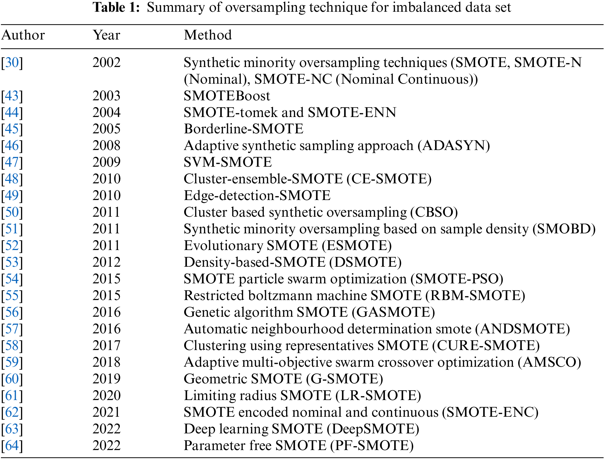
SMOTE oversampling technique only works for the dataset with all continuous features. SMOTE-Nominal and Continuous (SMOTE-NC) can be used for a dataset with a mix of categorical and continuous features. SMOTEBoost [43], SMOTE-Tomek, SMOTE-ENN [44], Borderline-SMOTE [45], Adaptive Synthetic (ADASYN) [46], and SMOTE-SVM [47] are some variants of SMOTE. A summary of some SMOTE techniques is given in Table 1.

Unlike the random oversampling (ROS) approach, the Synthetic Minority Oversampling Techniques (SMOTE) and SMOTEBoost were developed to perform more intelligent oversampling or improvised ROS. SMOTE, proposed by Chawla et al. [30], solved the limitation of ROS, an over-fitting issue, by generating artificial instances in the minority class using the concept of interpolation and the k-nearest neighbour technique, as shown in Fig. 1.

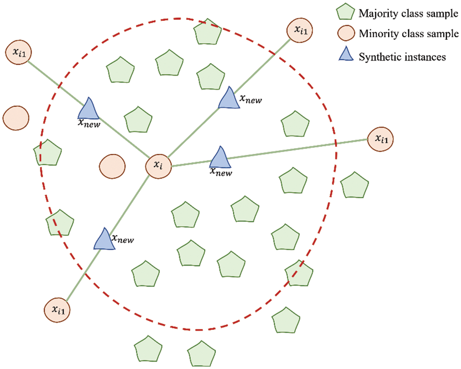
Figure 1: An illustration of how to generate artificial instances using SMOTE algorithm

A xi positive instance from the minority class is selected to generate new synthetic data points. Then, based on a distance metric, several Nearest Neighbor (NN) of the same class (points xi1 to xi4) are chosen from the training set. Finally, a randomized interpolation is carried out to obtain new instances r1 to r4.

The flow of SMOTE algorithm starts with setting the total amount of oversampling N. Next, an iterative process is carried out which is composed of several steps. First, a positive instance from a minority class is selected at random from the training set. Then, its k-NN is obtained. Finally, N of these k instances are randomly chosen to compute the new instances by interpolation. The difference between the feature vector (sample) under consideration and each neighbour is taken. This difference is multiplied by a random number drawn between 0 and 1, and then added to the previous feature vector. SMOTE generates instances only within or between the available examples and never creates instances outside the border. Therefore, SMOTE never creates new regions of minority instances. This approach was found considerably effective in handling the issue of oversampling in an imbalanced dataset using C4.5 as the classifier [43].

Despite the limitations, SMOTE overcomes random oversampling by generalizing the decision region for the minority class as it does not necessarily cause over-fitting [30]. The success of SMOTE has led to new variants, such as borderline-SMOTE, in which only instances close to the borderline or decision boundary are chosen for oversampling [45]. This approach differs from the existing oversampling, in which all minority examples or random subsets of the minority class are oversampled.

Batista et al. [44] presented another upscale method, hybridizations of undersampling and oversampling, where SMOTE is a hybrid with the Tomek Link (TLink) approach. This method works as follows: SMOTE was used to oversample the minority class. Then, the TLink approach was used to detect and eliminate the redundant observations in the majority class. This approach has shown promising results in handling imbalanced datasets. Then, [44] proposed SMOTE-ENN, which generated synthetic examples for the minority class and then used ENN (Edited Nearest Neighbour) method to delete some observations that have different classes between the observation’s class and its K-nearest neighbours majority class. The Edited-Nearest Neighbor (ENN) method first finds the k-nearest neighbour of each observation and then checks whether the majority class from the observation’s k-nearest neighbour is the same as the observation’s class or not. If the majority class of the observation’s K-nearest neighbour and the observation’s class are different, then the observation and its K-nearest neighbour are deleted from the dataset. By default, the number of nearest neighbours used in ENN is k = 3. Thus, SMOTE-ENN combined the SMOTE ability to generate synthetic examples for minority class and ENN ability to delete some observations, thus producing better synthetic samples. Meanwhile, SVM-SMOTE [47] balances class distribution by generating new minority class instances near borderlines with SVM. Here, the SVM algorithm was used instead of k-NN to identify misclassified examples on the decision boundary.

Due to imbalanced data, failure prediction has evolved to hybrid methods, such as combining sampling techniques with machine learning classifiers. It is important to understand the type of data (nominal or continuous) that can be used for SMOTE and variants of SMOTE techniques.

2.2 Logistic Regression

Logistic Regression (LR) is one statistical model for classifying a binary (0, 1) dependent variable. The event of interest is Y = 1 and 0 otherwise, such as Y = 1(failure) and Y = 0 (non-failure). The independent variables can be a mixture of nominal, ordinal, or continuous variables. In simple mathematical form, the logistic regression model [65] with k independent variable is written as:

log⁡[p1−p]=β0+β1X1+β2X2+⋯+βkXk(1)

where p=P(Y=1) is the probability of the event occurring, β0 is the intercept, βj is the coefficient for Xj, j=1,2,3,…,k.Xj which are the predictor or independent variables. The predicted class of a case (or customer) is 1 if p(Y=1)>0.5, otherwise the predicted class is 0. The odds-ratio (eβ^j) provides information on the effect of Xj on the event Y=1. If the odds-ratio for a continuous independent variable is greater than 1 then the likelihood of event Y=1 increases as X increases. The odds ratio for a binary categorical independent variable (A,B) is the ratio of two odds: p1−pq1−q or p(1−q)q(1−p). If the odds-ratio is greater than, the odd of failure is higher for pump A, and if the odds-ratio is less than 1, the odds of failure is higher for pump B. If the odds-ratio is equal to 1, then the odd of failure is equally likely for both pumps. p is the proportion of failure for pump A while q is the proportion of failure for pump B.

The simulation study by [4] showed that the imbalanced data affected the parameter estimate of the logistic regression model. The severity of imbalance on parameter estimates of the logistic regression model depends on sample size and imbalance ratio (IR). The estimates are biased for IR less than 30%, 20%, and 10% when the sample size is 100, 500, and 1000 respectively. While for larger samples, the estimates are biased when IR is 5% and below. Machine learning techniques such as logistic regression, decision trees, naïve bayes, and support vector machines have low sensitivity when imbalanced data [14].

2.3 Naïve Bayes and Gaussian Naïve Bayes

Naïve Bayes is a classification technique based on Bayes Theorem with an assumption of independence among predictors. Naïve Bayes involves the calculation of the posterior probability P (Y|X) from P(Y), P(X|Y), and P(X) [66,67]. The Y is the dependent or target variable, and X is the independent variable. The Y and X must be categorical variables. Thus, the algorithm will convert the continuous variable into categorical variables.

The posterior probability of Y given X is then calculated as follows [67]:

P(Y|X)=P(X|Y)⋅P(Y)P(X)(2)

where:

Y = Target variable or class for which the case i belongs

P(Y|X)= Probability of Y given information on X

P(Y)= Prior probability for Y

P(X|Y)= Probability X given information on Y

P(X)= Probability of X

For k covariates, the posterior probability is obtained as follows:

P(Y|X1X2…Xk)=P(X1X2…Xk|Y)P(Y)P(X1X2…Xk)

However, Gaussian Naïve Bayes (GNB) is used when the independent variables are continuous, and we do not wish to convert them into categories. GNB assumes that X follows a Gaussian or normal distribution and requires the mean and variance of X for class c of Y.

For a given feature value X, the probability density assuming that X is in a category C is P(X|C)∼N(μc,σc2), where P(X|Y=c)∼12πσ2e−(x−μc)22σ2. The estimate of probability for observation (x1,x2,…,xn) as the product of the densities P((x1,x2,…,xn)|cj)∼N(x1,μ1c,σ1c2,…,xn,μnc,σnc2). Then the Bayes formula to invert the conditional probabilities is P(cj|(x1,x2,…,xn))=P((x1,x2,…,xn)|cj)P(cj)P(x1,x2,…,xn). However, the denominator does not depend on the category cj, thus P(cj|(x1,x2,…,xn))∼P((x1,x2,…,xn)|cj)P(cj). Then the highest value is selected from this equation [67].

2.4 Support Vector Machine

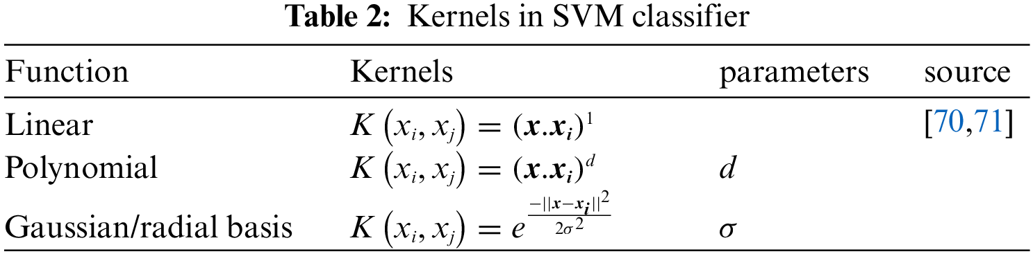
Cortes et al. [68] introduced the Support Vector Machine (SVM) for classification problems. Support vector machines (SVM) are based on statistical learning theory and belong to the class of kernel-based methods. It can handle the classification of linear and non-linear separation. SVM algorithm attempts to find a linear separator (or hyperplane) between the data points of two classes in multidimensional space. Such a hyperplane is called the optimal hyperplane. A set of instances closest to the optimal hyperplane is called a support vector. Finding the optimal hyperplane provides a linear classifier. SVMs are well suited for dealing with interactions among features and redundant features [69]. There are a few kernels in SVM types, including linear, polynomial, sigmoid and radial basis function (RBF). Table 2 lists the kernel functions commonly used in SVM applications for classification problems [67].

For a binary classification problem shown in Fig. 2, the decision boundary of a linear classifier is written as: w.x + b = 0, where w and b are the model’s parameters.

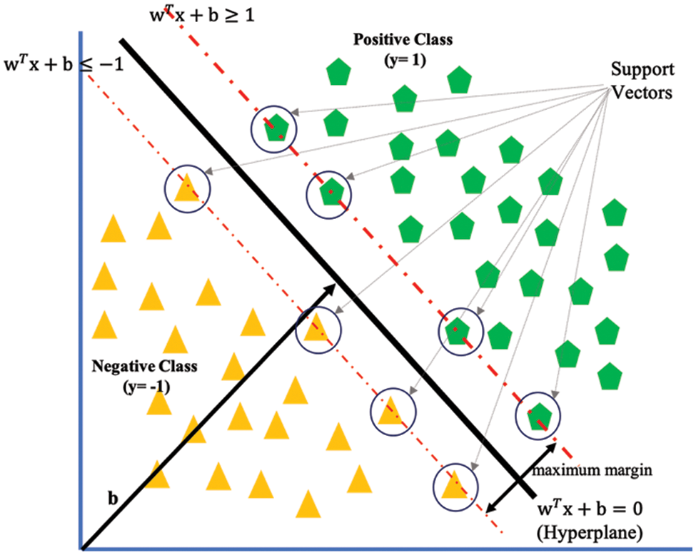
Figure 2: SVM hyperplane for binary classification

The case z is classified as follows:

y=f(x)={1,if w.z+b>0−1,if w.z+b<0

where z=x+b. Furthermore, the SVM can be formulated as an optimization which maxw=2||2|| subject to wTxi+b {≥1 if yi=+1≤−1 if yi=−1

This is a quadratic optimization problem subject to linear constraints and is known as a convex optimization problem and can be solved using the Lagrange multiplier method [67].

The radial basis is the most preferred and used kernel functions in SVM. It is usually chosen for non-linear data. It helps to make proper separation when there is no prior knowledge of data.

In general, given a training set of N data points {yk,xk}k=1N, where xk∈Rn is the kth input pattern and yk∈R is the kth output pattern, the support vector method approach aims at constructing a classifier of the form:

y(x)=sign[∑k=1NakykΨ(x,xk)+b](3)

where ak are positive real constants and b is a real constant. The kernel for SVM are: Ψ(x,xk)=xkTx (linear SVM); Ψ(x,xk)=(xkTx+1)d (polynomial SVM of degree d); Ψ(x,xk)=exp {−∥x−xk ∥22/σ2} (RBF SVM); Ψ(x,xk)=tanh [KxkTx+θ]  (two layer neural SVM), where σ, K and θ are constants [67,72].

The classifier is constructed as follows. One assumes that

{wTφ(xk)+b≥1, wTφ(xk)+b≤−1, {if yk=+1if yk=−1(4)

which is equivalent to

yk[wTφ(xk)+b]≥1=1,…,N(5)

where φ(⋅) is a nonlinear function which maps the input space into a higher dimensional space [67].

3  Methodology

In this paper, we use a cleaned sample of time series data called the Produced Water Re-injection (PWRI) dataset, which was obtained with permission from a local Oil and Gas company in Malaysia for research purposes. The aim is to develop a predictive model for machine failure prediction. The minority class (failure) only made up 3% of the total sample data, resulting in a severely imbalanced dataset. When data is imbalanced, the machine learning algorithm usually ignores the proportion of the negative classes and predicts 97% accuracy, but only based on “non-failure.” Hence, machine learning will have very low or zero sensitivity as it will fail to classify the minority samples. The methodology flowchart is presented in Fig. 3.

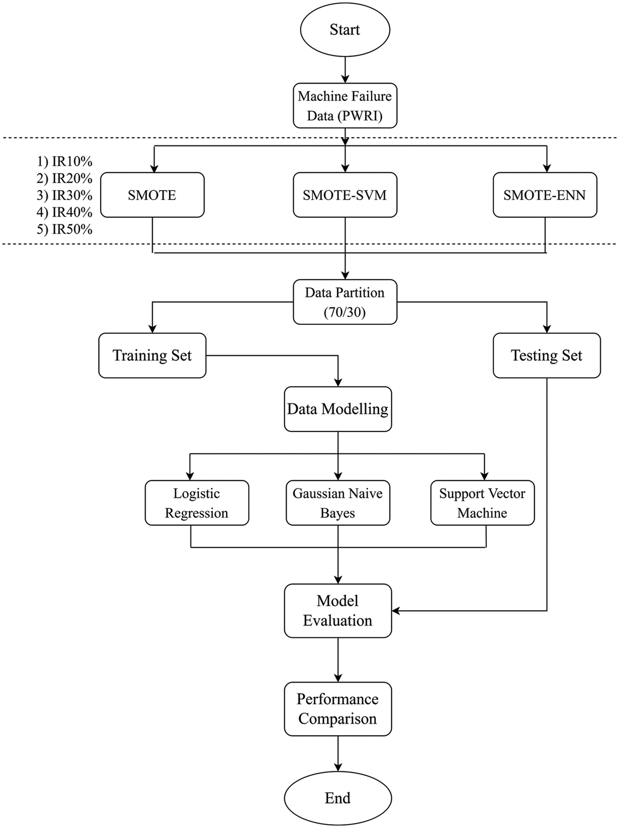
Figure 3: Flowchart of research process

3.1 Description of Variables

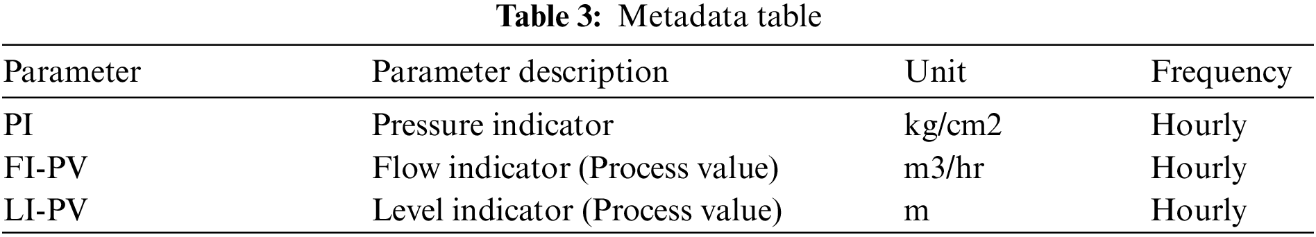
The dataset consists of three continuous independent variables which are Pressure Indicator (PI), Flow Indicator (FI), and Level Indicator (LI) and one dependent variable which is failure status (Failure/Non-Failure). The data are hourly data collected from the pump system as in Table 3.

The original dataset consists of 20,473 which is made up of 19,945 ‘non-failure’ data and 528 ‘failure data’. The data was highly imbalanced, with a ratio of 97:3 in terms of percentage.

3.2 Creating Data Sets Using SMOTE, SMOTE-SVM and SMOTE-ENN

Using the original imbalance date, we used the SMOTE technique to create “synthetic” examples of the minority samples. The minority class is over-sampled by taking each minority class sample and introducing synthetic examples along the line segments joining any or all of the k-minority class nearest neighbours. From the original imbalanced dataset, using SMOTE, we create different sets of imbalanced data with 10%, 20%, 30%, 40%, and 50% failure class proportions. This process of creating datasets with different imbalance ratios was repeated using SMOTE-SVM and then SMOTE-ENN. The proportion of failure and non-failure samples for the five different datasets generated is shown in Table 4.

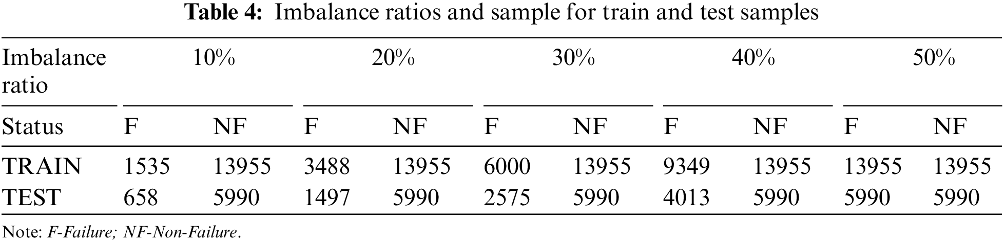
Each of the five datasets with different imbalanced ratios generated was partitioned randomly into 70% training and 30% testing samples, and the sample size details are shown in Table 4.

In the model development and evaluation stage, the three classifiers (logistic regression, Gaussian Naïve Bayes, and Support Vector Machine using RBF kernel) were developed using the training sample and validated using the testing sample. The classifiers were then evaluated based on accuracy, sensitivity, specificity, precision, and F-Measure.

3.3 Classification Performance Measures

The classifiers were evaluated based on accuracy, sensitivity, specificity, precision, and F-measure. The confusion matrix in Table 5 was used to obtain the accuracy, sensitivity, specificity, precision, and F-Measure.

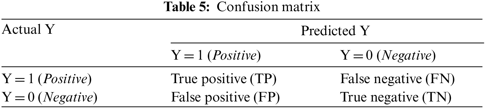
The true positive indicates positive cases predicted correctly, while the false positive indicates negative cases predicted incorrectly. Similarly, the true negative is the negative case predicted correctly, while the false negative is the positive case predicted incorrectly. In summary,

Accuracy (proportion of cases which are accurately predicted)=TP+TNTP+FP+TN+FN

Sensitivity (proportion of positive cases that are correctly predicted)=TPTP+FN

Specificity (proportion of negative cases that are correctly predicted)=TNTN+FP

Precision (proportion of predicted positive cases that are actual positives)=TPTP+FP

F−measure =2∗(Precision∗Recall)Precision∗Recall

4  Results and Discussion

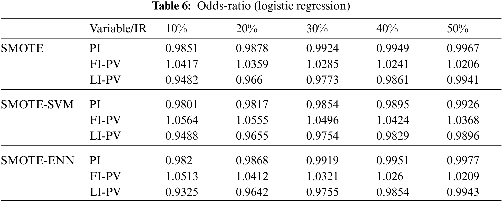
The section presents the results and findings of the study. The logistic regression results (Table 6) for the original data show that all variables are significant predictors of machine failure. Machine failure is more likely to occur when pressure indicator (PI) (b1 = −0.0149) and Level Indicator (b3 = −0.0897) decreases, and when Flow Indicator increases (b2 = 0.0401). The odds-ratios using exp (b) are 0.9852, 1.0409 and 0.9142 respectively. Similar findings were obtained when logistic regression models were developed using the data which was balanced using SMOTE, SMOTE-SVM, and SMOTE-ENN. The results in Table 6 confirmed that the imbalanced ratio of logistic regression affects the coefficients and odds ratio. The odds-ratio value changes when the imbalance rate changes. The odds-ratio was obtained using the exponentiation of the coefficients [4].

We then compared the performance of the three models (Model 1: Gaussian Naïve Bayes, Model 2: Logistic Regression and Model 3: SVM). The classifier performance results using SMOTE are shown in Table 7. The Receiver Operating Characteristic (ROC) curves in Fig. 4 illustrate the classifier performance under SMOTE. The green curve for model 3 (SVM) is higher than the blue curve (Model 2: logistic regression) and orange curve (Model 1: GNB). SVM (RBF) has higher sensitivity for IR 30% and above. Under SMOTE, Naïve Bayes has higher sensitivity when data IR is 10% and 20%, while SVM has higher sensitivity than NB and logistic regression when IR is 30% and above. Next, we compared the performance of the classifiers under different SMOTE techniques.

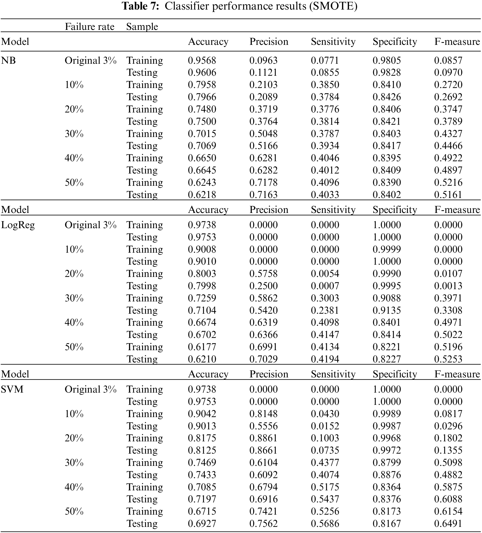
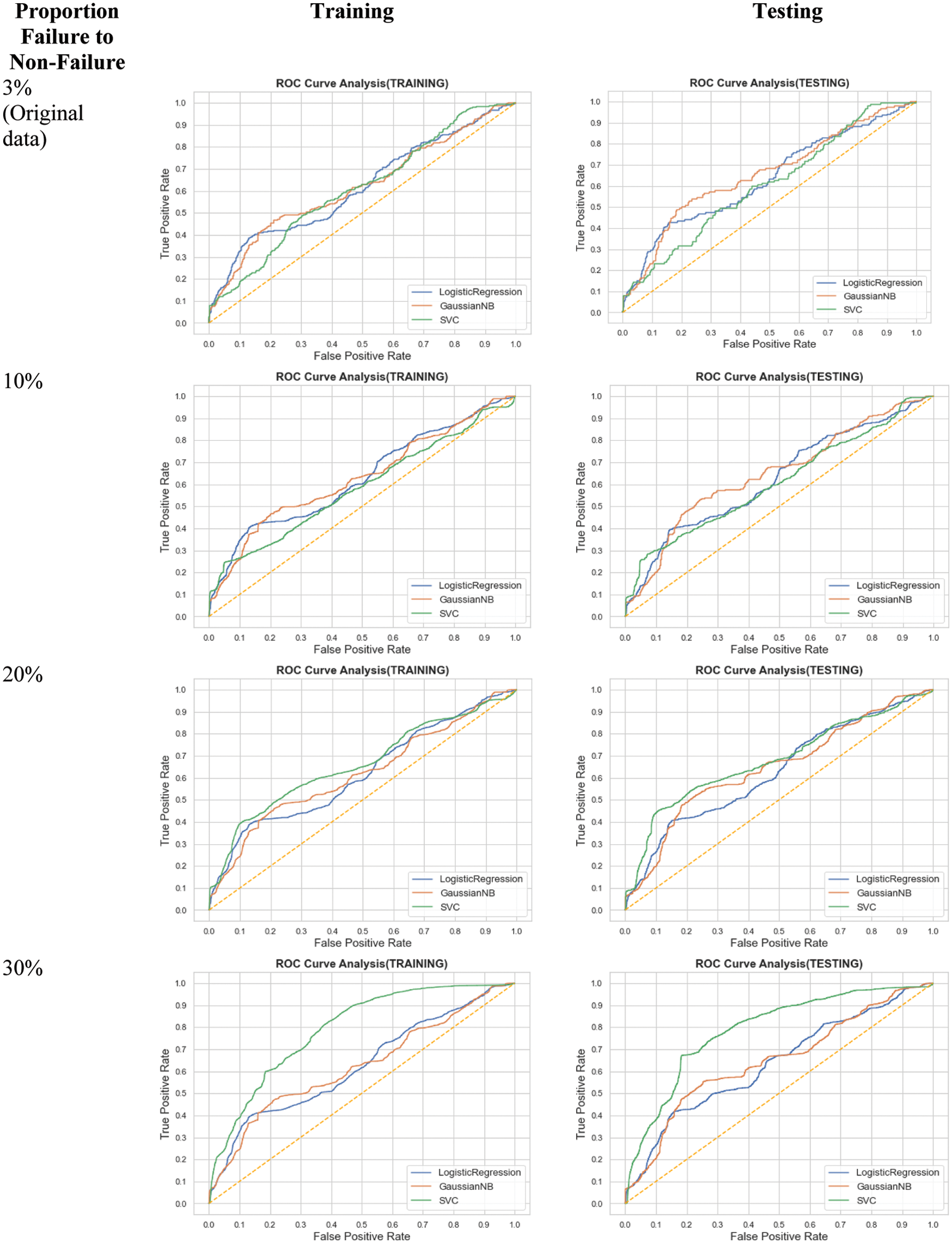
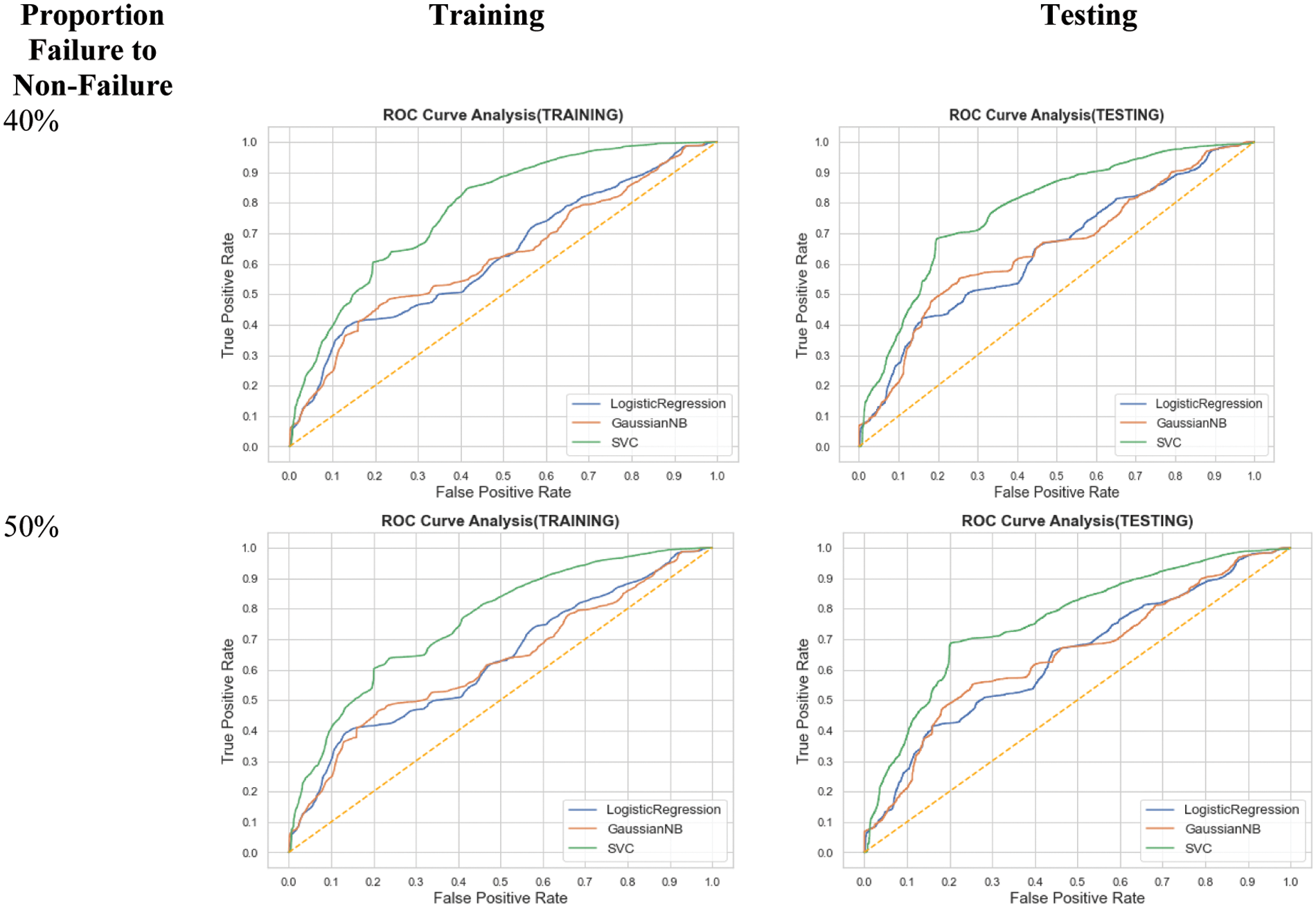
Figure 4: ROC curves for different imbalance ratios using SMOTE

The spider chart in Fig. 5 and bar chart in Figs. 6–8 show the machine learning performance for three types of SMOTE. The spider chart in Fig. 5 and bar chart in Fig. 6 show that NB consistently has higher sensitivity and F-measure under SMOTE-SVM. The sensitivity and F-measure for logistic regression (Fig. 7) and SVM (Fig. 8) are higher under SMOTE-SVM except when IR is 30% where the performance is higher under SMOTE-ENN.

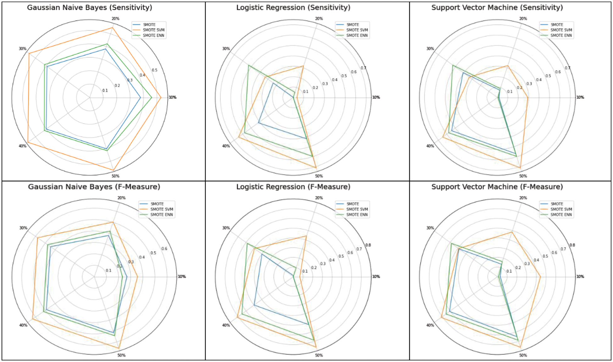
Figure 5: Classifier performance for different SMOTE techniques

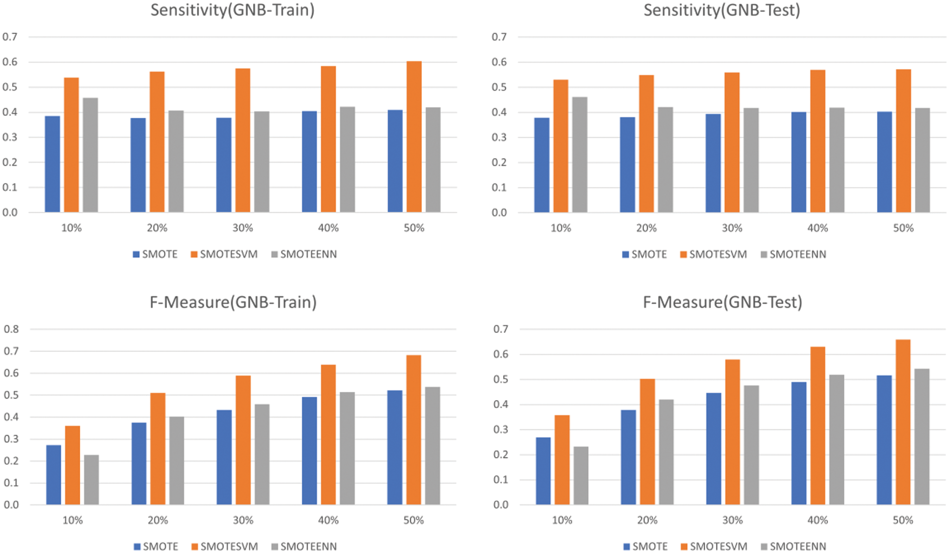
Figure 6: GNB performance using SMOTE, SMOTE-SVM and SMOTE-ENN

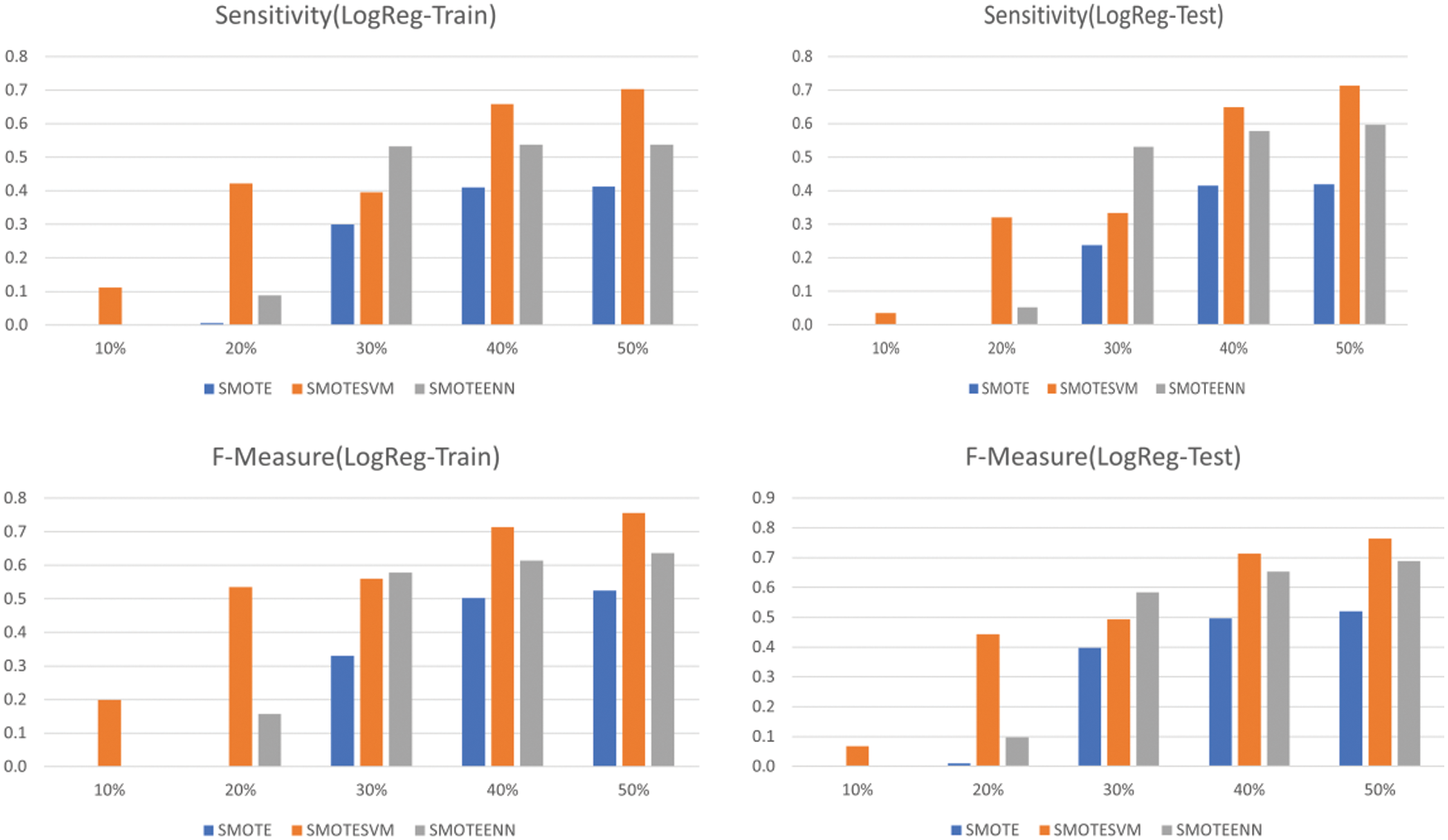
Figure 7: Logistic regression performance using SMOTE, SMOTE-SVM and SMOTE-ENN

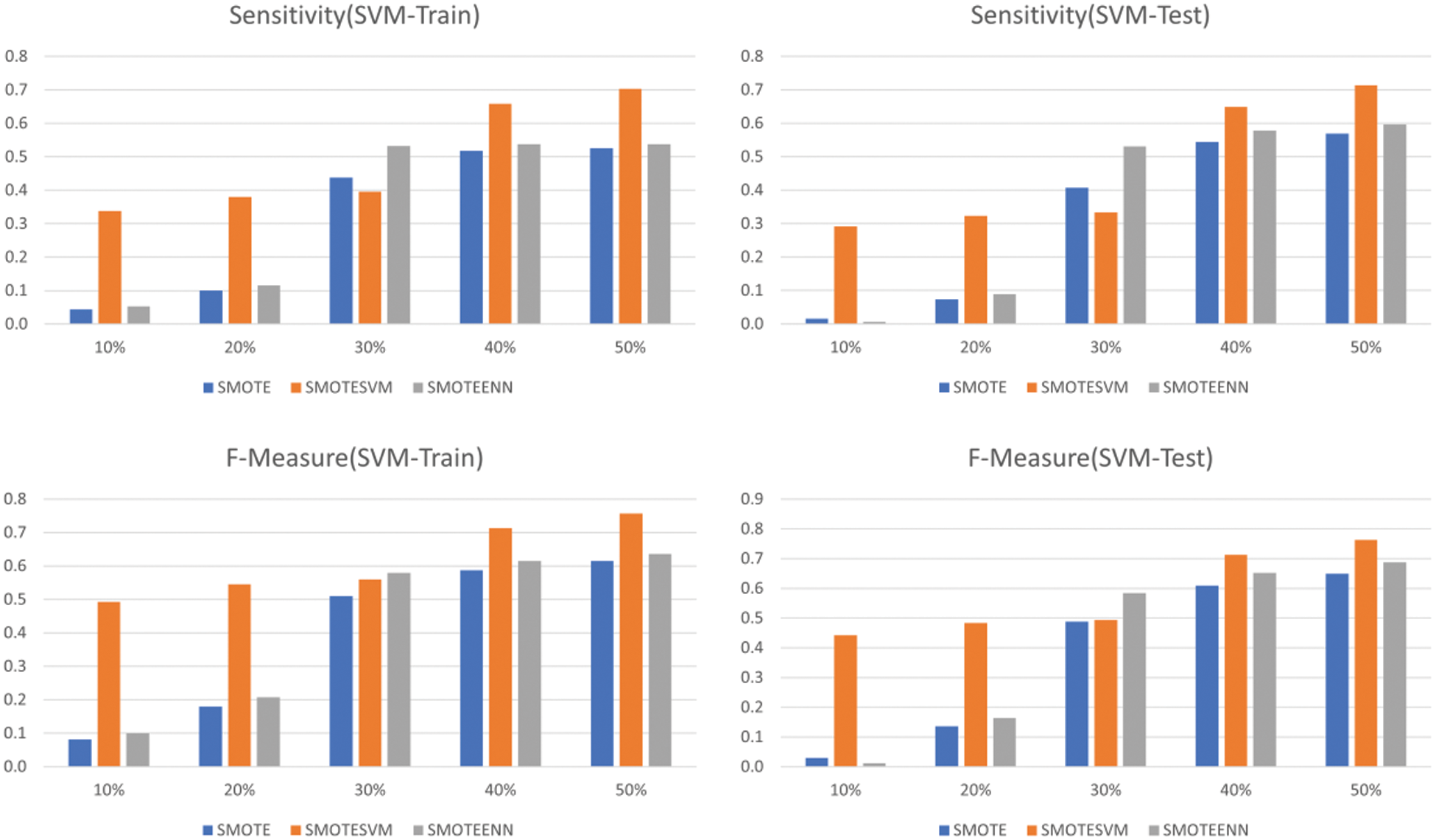
Figure 8: SVM performance using SMOTE, SMOTE-SVM and SMOTE-ENN

Overall, SVM (RBF) under SMOTE-SVM has higher performance than GNB and LogReg when IR is 30% and above. Results of this study support that SMOTE techniques especially can improve classifiers’ performance for imbalanced data [9–10,73,74]. There is also no overfitting issue It is important to note that SMOTE tends to oversample uninformative samples or noisy samples [73] while SMOTE-ENN could delete noisy samples [44,74]. The advantage of SMOTE-SVM [47] is that it focuses on generating new minority class instances near borderlines with SVM and thus produces better synthetic samples when balancing the data.

5  Conclusion

This paper investigates the performance of logistic regression Gaussian Naïve Bayes and Support Vector Machine using the SMOTE technique to balance data imbalance for machine failure prediction. Results showed that Gaussian Naïve Bayes consistently improves sensitivity and precision as the imbalance ratio increases from 10% to 50% under SMOTE. However, the sensitivity of Gaussian Naïve Bayes is still below 50% when data is balanced. Logistic regression and SVM have close to zero sensitivity when IR is 10% and 20%. The sensitivity and F-measure for SVM are higher than GNB and Logistic regression when IR is 30% to 50%. Regarding evaluation of SMOTE techniques, the sensitivity and F-measure for the logistic regression model and SVM are higher under SMOTE-SVM except when the imbalance rate is 30%, where performance is higher using SMOTE-ENN. The SVM sensitivity and F-measure are the highest for SMOTE-SVM and lowest under SMOTE, while for Gaussian Naïve Bayes, the sensitivity and F-measure are consistently higher under SMOTE-SVM. This study has shown that SMOTE-SVM is a good oversampling technique to improve classifier performance for imbalanced data with continuous features. The advantage of SMOTE-SVM is that it focuses on generating new minority class instances near borderlines with SVM and thus produces better synthetic samples. Future work will involve simulation studies to verify these findings and investigate SMOTE techniques for the dataset with categorical and continuous features.

Acknowledgement: The authors thank CerDaS (Centre for Research in Data Science), University Teknologi PETRONAS and IBDAAI (Institute for Big Data Analytics and Artificial Intelligence), UiTM for this project collaboration. We also thank the reviewers for the comments which contribute to the improvement of the article.

Funding Statement: This study was supported under the research Grant (PO Number: 920138936) from the Institute of Technology PETRONAS Sdn Bhd, 32610, Bandar Seri Iskandar, Perak, Malaysia.

Conflicts of Interest: The authors declare that they have no conflicts of interest to report regarding the present study.

References

1. N. V. Chawla, N. Japkowicz and A. Kolcz, “Editorial: Special issue on learning from imbalanced data sets,” ACM Special Interest Group on Knowledge Discovery and Data Mining (SIGKDD) Explorations Newsletter, vol. 6, no. 1, pp. 1–6, 2004. [Google Scholar]

2. H. He and E. A. Garcia, “Learning from imbalanced data,” IEEE Transactions on Knowledge and Data Engineering, vol. 21, no. 9, pp. 1263–1284, 2009. [Google Scholar]

3. G. M. Weiss and F. Provost, “Learning when training data are costly: The effect of class distribution on tree induction,” Journal of Artificial Intelligence Research, vol. 19, pp. 315–354, 2003. [Google Scholar]

4. H. A. A. Rahman, Y. B. Wah and O. S. Huat, “Predictive performance of logistic regression for imbalanced data with categorical covariate,” Pertanika Journal of Science and Technology, vol. 29, no. 1, pp. 181–197, 2021. [Google Scholar]

5. B. Mohammed, I. Awan, H. Ugail and M. Younas, “Failure prediction using machine learning in a virtualised HPC system and application,” Cluster Computing, vol. 22, no. 2, pp. 471–485, 2019. [Google Scholar]

6. N. Rücker, L. Pflüger and A. Maier, “Hardware failure prediction on imbalanced times series data: Generation of artificial data using Gaussian process and applying LSTMFCN to predict broken hardware,” Journal of Digital Imaging, vol. 34, no. 1, pp. 182–189, 2021. [Google Scholar]

7. M. Hanafy and R. Ming, “Machine learning approaches for auto insurance big data,” Risks, vol. 9, no. 2, pp. 1–23, 2021. [Google Scholar]

8. A. K. I. Hassan and A. Abraham, “Modeling insurance fraud detection using imbalanced data classification,” in Advances in Nature and Biologically Inspired Computing, vol. 419. Switzerland: Springer, Cham, pp. 117–127, 2016. [Google Scholar]

9. S. S. Kotekani and I. Velchamy, “An effective data sampling procedure for imbalanced data learning on health insurance fraud fetection,” Journal of Computing and Information Technology, vol. 28, no. 4, pp. 269–285, 2020. [Google Scholar]

10. S. Fotouhi, S. Asadi and M. W. Kattan, “A comprehensive data level analysis for cancer diagnosis on imbalanced data,” Journal of Biomedical Informatics, vol. 90, pp. 1–30, 2019. [Google Scholar]

11. B. Song, S. Li, S. Sunny, K. Gurushanth, P. Mendonca et al., “Classification of imbalanced oral cancer image data from high-risk population,” Journal of Biomedical Optics, vol. 26, no. 10, pp. 1–9, 2021. [Google Scholar]

12. B. Zhu, B. Baesens and S. K. L. M. Vanden Broucke, “An empirical comparison of techniques for the class imbalance problem in churn prediction,” Information Sciences, vol. 408, pp. 84–99, 2017. [Google Scholar]

13. R. Soleymani, E. Granger and G. Fumera, “Progressive boosting for class imbalance and its application to face re-identification,” Expert System with Applications, vol. 101, pp. 271–291, 2018. [Google Scholar]

14. N. A. M. Salim, Y. B. Wah, C. Reeves, M. Smith, W. F. W., Yaacob et al., “Prediction of dengue outbreak in selangor Malaysia using machine learning techniques,” Scientific Reports, vol. 11, no. 1, 939, pp. 1–9, 2021. [Google Scholar]

15. A. Fernández, S. García, M. Galar, R. C. Prati, B. Krawczyk et al., “Imbalanced classification for big data,” in Learning from Imbalanced Datasets, Berlin, Germany: Springer, 2018. [Google Scholar]

16. E. A. Pakhir and N. Ayuni, “Predictive analytics of machine failure using linear regression on KNIME platform,” in Proc. of IEEE Int. Conf. on Artificial Intelligence and Virtual Reality (AAIVR 2021), Kumamoto, Japan, pp. 59–64, 2021. [Google Scholar]

17. M. S. Diallo, S. A. Mokeddem, A. Braud, G. Frey and N. Lachiche, “Identifying benchmarks for failure prediction in industry 4.0,” Informatics, vol. 8, no. 4, pp. 1–13, 2021. [Google Scholar]

18. K. Guo, J. Zhao and Y. Liang, “Flow shop failure prediction problem based on grey-markov model,” Personal and Ubiquitous Computing, 2021. https://doi.org/10.1007/s00779-021-01618-0 [Google Scholar] [CrossRef]

19. J. Lee, W. Choi and J. Kim, “A cost-effective CNN-LSTM-based solution for predicting faulty remote water meter reading devices in AMI systems,” Sensors, vol. 21, no. 18, pp. 1–20, 2021. [Google Scholar]

20. W. Lee and K. Seo, “Early failure detection of paper manufacturing machinery using nearest neighbor-based feature extraction,” Engineering Reports, vol. 3, no. 2, pp. 1–19, 2021. [Google Scholar]

21. S. Sridhar and S. Sanagavarapu, “Handling data imbalance in predictive maintenance for machines using SMOTE-based oversampling,” in Proc. of 2021 IEEE 13th Int. Conf. on Computing Intelligence and Communication Networks (CICN 2021), Lima, Peru, pp. 44–49, 2021. [Google Scholar]

22. A. C. M. Silveira, Á. Sobrinho, L. Dias and E. D. B. Costa, “Exploring early prediction of chronic kidney disease using machine learning algorithms for small and imbalanced dataset,” Applied Sciences, vol. 12, no. 7, pp. 1–25, 2022. [Google Scholar]

23. A. M. Sowjanya and O. Mrudula, “Effective treatment of imbalanced datasets in health care using modified SMOTE coupled with stacked deep learning algorithms,” Applied Nanoscience, vol. 12, pp. 1–12, 2022. [Google Scholar]

24. W. Chaipanha and P. Kaewwichian, “Smote vs. random undersampling for imbalanced data-car ownership demand model,” Communications-Scientific Letters of the University of Zilina, vol. 24, no. 3, pp. 105–115, 2022. [Google Scholar]

25. S. Demir and E. K. Şahin, “Evaluation of oversampling methods (OVER, SMOTE, and ROSE) in classifying soil liquefaction dataset based on SVM, RF, and Naïve Bayes,” European Journal of Science and Technology, no. 34, pp. 142–147, 2022. [Google Scholar]

26. M. Muntasir Nishat, F. Faisal, I. Ratul, A. Al-Monsur, A. M. Ar-Rafi et al., “A comprehensive investigation of the performances of different machine learning classifiers with SMOTE-ENN oversampling technique and hyperparameter optimization for imbalanced heart failure dataset,” Scientific Programming, vol. 2022, pp. 1–17, 2022. [Google Scholar]

27. T. Nguyen, R. G. Gosine and P. Warrian, “A systematic review of big data analytics for oil and gas industry 4.0,” IEEE Access, vol. 8, pp. 61183–61201, 2020. [Google Scholar]

28. P. Bangert, Machine Learning and Data Science in the oil and gas Industry: Best Practices, Tools, and Case Studies. Texas, USA: Gulf Professional Publishing, Elsevier, 2021. [Google Scholar]

29. H. Wang, W. Lu, S. Tang and Y. Song, “Predict industrial equipment failure with time windows and transfer learning,” Applied Intelligence, vol. 52, no. 3, pp. 2346–2358, 2022. [Google Scholar]

30. N. V. Chawla, K. W. Bowyer, L. O. Hall and W. P. Kegelmeyer, “SMOTE: Synthetic minority over-sampling technique,” Journal of Artificial Intelligence Research, vol. 16, pp. 321–357, 2002. [Google Scholar]

31. J. Pesantez-Narvaez, M. Guillen and M. Alcañiz, “Predicting motor insurance claims using telematics data—XGboost versus logistic regression,” Risks, vol. 7, no. 2, pp. 1–16, 2019. [Google Scholar]

32. Y. Freund and R. E. Schapire, “A decision-theoretic generalization of on-line learning and an application to boosting,” Journal of Computer and System Sciences, vol. 55, no. 1, pp. 119–139, 1997. [Google Scholar]

33. W. Wang and D. Sun, “The improved adaboost algorithms for imbalanced data classification,” Information Sciences, vol. 563, pp. 358–374, 2021. [Google Scholar]

34. W. Fan, S. J. Stolfo, J. Zhang and P. K. Chan, “AdaCost: Misclassification cost-sensitive boosting,” in Proc. of the Sixteenth Int. Conf. on Machine Learning (ICML’99), Bled, Slovenia, vol. 99, pp. 97–105, 1999. [Google Scholar]

35. H. Bei, Y. Wang, Z. Ren, S. Jiang, K. Li et al., “A statistical approach to cost-sensitive AdaBoost for imbalanced data classification,” Mathematical Problems in Engineering, vol. 2021, pp. 1–20, 2021. [Google Scholar]

36. K. M. Ting, “A comparative study of cost-sensitive boosting algorithms,” in Proc. of the 17th Int. Conf. on Machine Learning, Stanford, USA, pp. 983–990, 2000. [Google Scholar]

37. Y. Sun, M. S. Kamel, A. K. C. Wong and Y. Wang, “Cost-sensitive boosting for classification of imbalanced data,” Pattern Recognition, vol. 40, no. 12, pp. 3358–3378, 2007. [Google Scholar]

38. N. V. Chawla, “Data mining for imbalanced datasets: An overview,” in Data Mining and Knowledge Discovery Handbook, Boston, MA, USA: Springer, pp. 875–886, 2009. [Google Scholar]

39. C. Pak, T. T. Wang and X. H. Su, “An empirical study on software defect prediction using over-sampling by SMOTE,” International Journal of Software Engineering and Knowledge Engineering, vol. 28, no. 6, pp. 811–830, 2018. [Google Scholar]

40. S. Barua, M. M. Islam, X. Yao and K. Murase, “MWMOTE-majority weighted minority oversampling technique for imbalanced data set learning,” IEEE Transactions on Knowledge and Data Engineering, vol. 26, no. 2, pp. 405–425, 2014. [Google Scholar]

41. E. Ramentol, Y. Caballero, R. Bello and F. Herrera, “SMOTE-RSB*: A hybrid preprocessing approach based on oversampling and undersampling for high imbalanced data-sets using SMOTE and rough sets theory,” Knowledge and Information Systems, vol. 33, no. 2, pp. 245–265, 2012. [Google Scholar]

42. J. A. Sáez, J. Luengo, J. Stefanowski and F. Herrera, “SMOTE-IPF: Addressing the noisy and borderline examples problem in imbalanced classification by a re-sampling method with filtering,” Information Sciences, vol. 291, pp. 184–203, 2015. [Google Scholar]

43. N. V. Chawla, A. Lazarevic, L. O. Hall and K. W. Bowyer, “SMOTEBoost: Improving prediction improving prediction of the minority class in boosting: Knowledge discovery in databases,” in Proc. of the 7th European Conf. on Principles and Practice of Knowledge Discovery in Databases, Cavtat-Dubrovnik, Croatia, pp. 107–119, 2003. [Google Scholar]

44. G. E. A. P. A. Batista, R. C. Prati and M. C. Monard, “A study of the behavior of several methods for balancing machine learning training data,” ACM Special Interest Group on Knowledge Discovery and Data Mining (SIGKDD) Explorations Newsletter, vol. 6, no. 1, pp. 20–29, 2004. [Google Scholar]

45. H. Han, W. Y. Wang and B. H. Mao, “Borderline-SMOTE: A new over-sampling method in imbalanced data sets learning,” Lecture Notes in Computer Science, vol. 3644, pp. 878–887, 2005. [Google Scholar]

46. H. He, Y. Bai, E. A. Garcia and S. Li, “ADASYN: Adaptive synthetic sampling approach for imbalanced learning,” in Proc. of Int. Joint Conf. on Neural Networks, Hong Kong, China, no. 3, pp. 1322–1328, 2008. [Google Scholar]

47. Y. Tang, Y. Q. Zhang and N. V. Chawla, “SVMs modeling for highly imbalanced classification,” IEEE Transactions on Systems, Man, and Cybernetics, Part B (Cybernetics), vol. 39, no. 1, pp. 281–288, 2009. [Google Scholar]

48. S. Chen, G. Guo and L. Chen, “A new over-sampling method based on cluster ensembles,” in 24th IEEE Int. Conf. on Advanced Information Networking and Applications Workshop, Perth, Australia, pp. 599–604, 2010. [Google Scholar]

49. Y. I. Kang and S. Won, “Weight decision algorithm for oversampling technique on class-imbalanced learning,” in Proc. of Int. Conf. on Control, Automation and Systems (ICCAS 2010), Gyeonggi-do, Korea, pp. 182–186, 2010. [Google Scholar]

50. S. Barua, M. M. Islam and K. Murase, “A novel synthetic minority oversampling technique for imbalanced data set learning,” in Lecture Notes in Computer Science, vol. 7063, pp. 735–744, 2011. [Google Scholar]

51. Q. Cao and S. Wang, “Applying over-sampling technique based on data density and cost-sensitive SVM to imbalanced learning,” in Proc. of 4th Int. Conf. on Information Management and Industrial Engineering (ICIII 2011), Shenzen, China, vol. 2, pp. 543–548, 2011. [Google Scholar]

52. T. Deepa and M. Punithavalli, “An E-SMOTE technique for feature selection in high-dimensional imbalanced dataset,” in Proc. of 3rd Int. Conf. on Electronics Computer Technology (ICECT 2011), Kanyakumari, India, vol. 2, pp. 322–324, 2011. [Google Scholar]

53. C. Bunkhumpornpat, K. Sinapiromsaran and C. Lursinsap, “DBSMOTE: Density-based synthetic minority over-sampling technique,” Applied Intelligence, vol. 36, no. 3, pp. 664–684, 2012. [Google Scholar]

54. J. Li, S. Fong and Y. Zhuang, “Optimizing SMOTE by metaheuristics with neural network and decision tree,” in Proc. of the 3rd Int. Symp. on Computational Business Intelligence (ISCBI 2015), Bali, Indonesia, pp. 26–32, 2015. [Google Scholar]

55. M. Zięba, J. M. Tomczak, and A. Gonczarek, “RBM-SMOTE: Restricted boltzmann machines for synthetic minority oversampling technique,” in Intelligent Information and Database Systems, Lecture Notes in Computer Science, 7th Asian Conf. (ACIIDS 2015), Bali, Indonesia, vol. 9011, pp. 377–386, 2015. [Google Scholar]

56. K. Jiang, J. Lu and K. Xia, “A novel algorithm for imbalance data classification based on genetic algorithm improved SMOTE,” Arabian Journal for Science and Engineering, vol. 41, no. 8, pp. 3255–3266, 2016. [Google Scholar]

57. J. Yun, J. Ha and J. S. Lee, “Automatic determination of neighborhood size in SMOTE,” in Proc. of the 10th Int. Conf. on Ubiquitous Information Management and Communications, Danang, Vietnam, pp. 1–8, 2016. [Google Scholar]

58. L. Ma and S. Fan, “CURE-SMOTE algorithm and hybrid algorithm for feature selection and parameter optimization based on random forests,” BMC Bioinformatics, vol. 18, no. 1, pp. 1–18, 2017. [Google Scholar]

59. J. Li, S. Fong, R. K. Wong and V. W. Chu, “Adaptive multi-objective swarm fusion for imbalanced data classification,” Information Fusion, vol. 39, pp. 1–24, 2018. [Google Scholar]

60. G. Douzas and F. Bacao, “Geometric SMOTE a geometrically enhanced drop-in replacement for SMOTE,” Information Sciences, vol. 501, pp. 118–135, 2019. [Google Scholar]

61. X. W. Liang, A. P. Jiang, T. Li, Y. Y. Xue and G. T. Wang, “LR-SMOTE–an improved unbalanced data set oversampling based on K-means and SVM,” Knowledge-Based System, vol. 196, pp. 1–10, 2020. [Google Scholar]

62. M. Mukherjee and M. Khushi, “Smote-ENC: A novel SMOTE-based method to generate synthetic data for nominal and continuous features,” Applied System Innovation, vol. 4, no. 1, pp. 1–12, 2021. [Google Scholar]

63. D. Dablain, B. Krawczyk and N. V. Chawla, “DeepSMOTE: Fusing deep learning and SMOTE for imbalanced data,” IEEE Transactions on Neural Networks and Learning Systems (Early Accesspp. 1–15, 2022. [Google Scholar]

64. Q. Chen, Z. Zhang, W. Huang, J. Wu and X. Luo, “PF-SMOTE: A novel parameter-free SMOTE for imbalanced datasets,” Neurocomputing, vol. 498, pp. 75–88, 2022. [Google Scholar]

65. D. W. Hosmer Jr, S. Lemeshow and R. X. Sturdivant, Applied Logistic Regression. New York, USA: John Wiley & Sons, Inc., 2013. [Google Scholar]

66. H. Kang, S. J. Yoo and D. Han, “Senti-lexicon and improved naive Bayes algorithms for sentiment analysis of restaurant reviews,” Expert Systems with Applications, vol. 39, no. 5, pp. 6000–6010, 2012. [Google Scholar]

67. P. N. Tan, M. Steinbach and V. Kumar, Introduction to Data Mining. New Delhi, India: Pearson Education, 2016. [Google Scholar]

68. C. Cortes and V. Vapnik, “Support-vector networks,” Machine Learning, vol. 20, no. 3, pp. 273–297, 1995. [Google Scholar]

69. J. Han, M. Kamber and J. Pei, Data Mining: Concepts and Techniques, the Morgan Kaufmann Series in Data Management Systems. Waltham MA, USA: Elsevier Inc, 2011. [Google Scholar]

70. G. F. Smits and E. M. Jordaan, “Improved SVM regression using mixtures of kernels,” in Proc. of the 2002 Int. Joint Conf. on Neural Networks, Honolulu, USA, vol. 3, pp. 2785–2790, 2002. [Google Scholar]

71. B. Schölkopf, K. Sung, C. J. C. Burges, F. Girosi, P. Niyogi et al., “Comparing support vector machines with Gaussian kernels to radial basis function classifiers,” IEEE Transactions on Signal Processing, vol. 45, no. 11, pp. 2758–2765, 1997. [Google Scholar]

72. M. Kuhn and K. Johnson, Applied Predictive Modeling. New York, USA: Springer, 2013. [Google Scholar]

73. Z. Jiang, T. Pan, C. Zhang and J. Yang, “A new oversampling method based on the classification contribution degree,” Symmetry, vol. 13, no. 2,194, pp. 1–13, 2021. [Google Scholar]

74. A. Puri, M. K. Gupta, “Improved hybrid Bag-boost ensemble with K-means-SMOTE–ENN technique for handling noisy class imbalanced data,” The Computer Journal, vol. 65, no. 1, pp. 124–138, 2022. [Google Scholar]