Deep Learning for Multivariate Prediction of Building Energy Performance of Residential Buildings

1  Introduction

The energy performance of buildings (EPB) has been focused on addressing energy waste, among other concerns, such as the environment. Appliances, such as heating, ventilation, and air conditioning (HVAC), have accounted for most of the energy consumption in buildings [1]. In Europe, the United States, and worldwide, building energy consumption accounts for 40%, 38.9%, and 30% of the energy used, respectively [2]. Moreover, the misuse of HVAC has culminated in about 40% waste of supplied energy in developing countries, such as Nigeria [3]. Therefore, it is paramount to consider the heating load (HL) and cooling load (CL) in building designs to ensure efficient energy.

Due to the long lifespan of buildings and the inability to effect certain changes after the structure is built, the initial design decision is highly crucial. Specifically, a proper thermal design can lead to significant operational cost savings with short investment returns [4–6]. The simulation of building characteristics is a reliable approach for estimating HL and CL, as many factors or a combination of characteristics results in different load requirements [7]. Moreover, the simulation results in EPB are highly accurate in reflecting the actual measurements [1]. However, simulation results vary across software packages [7]. Simulations are complicated and time-consuming because they require user expertise for particular software and domain knowledge for parameter settings [1]. Machine and deep learning advancements have developed more accurate forecasting models for building energy demands using simulation data [8,9].

The artificial intelligence (AI) model has proved to be a reliable approach to effectively predict EPB, as AI models can analyze the significance of input parameters and offer solutions faster. There are two types of predictions: univariate and multivariate regressions [10]. A single variable is predicted as output from the model in univariate regression. Many efforts have been made to apply univariate prediction models to predict EPB. For instance, the nonlinear and nonparametric method, random forest (RF), has been compared with a classical linear regression approach to estimating the HL and CL [1]. The RF exhibits superior ability in the prediction of HL and CL. The genetic programming–based framework has also been proposed to estimate the EPB [11]. Genetic programming was blended with a local search method and linear scaling. The framework recorded a mean squared error (MSE) of 0.47 and 3.33 for HL and CL, respectively.

A tree-based ensemble learning algorithm has also been proposed for EPB prediction [12]. The algorithm with gradient-boosted regression trees (GBRT) among the RF and extremely randomized trees or extra trees recorded the lowest MSE of 0.1 and 0.3 for the HL and CL, respectively. Moreover, AI has been proposed to model HL and CL in building design. The study found that the ensemble approach using support vector regression (SVR) and the artificial neural network resulted in a good model with absolute percentage errors below 4% [2]. Other models investigated for the prediction of the EPB include the extreme learning machine (ELM), multivariate adaptive regression spline (MARS), and a hybrid model of MARS and ELM [13]. In the hybrid model, the MARS reduced the computational time needed for ELM by determining the most relevant input parameters required by ELM to make predictions. The hybrid model recorded a better average MSE performance of 0.0204 against MARS and ELM at 0.0240 and 0.8334, respectively. Bilous et al. [14] developed a regression model–based building energy performance tool for temperature prediction based on internal (e.g., HL) and external (e.g., ambient temperature) factors. In addition, deep learning has been used for building energy prediction. Amarasinghe et al. [15] proposed a convolutional neural network (CNN) and bidirectional long short-term memory for feature extraction and energy prediction in a time-series dataset. The model recorded significant improvement in energy prediction, but the model is designed for existing buildings with an energy consumption history.

In contrast, multivariate regression (also known as multi-output regression, multitarget, or multiresponse regression) aims to simultaneously predict multiple actual output/target variable values [10]. Depending on the output variable, the problem can be called multilabel classification in the case of binary output or multidimensional classification in the case of discrete output. The multivariate method has been applied to energy-related problems [9]. For instance, a multivariate linear regression model was employed to estimate the expected reduction in energy use intensity due to changes in operating hours, the number of occupants, U-values of walls, lighting, and the climate zone [16]. In addition, multi-input multi-output architecture was proposed for the time-series prediction of wind power generation and temperature using deep learning [17].

The CNN for multivariate prediction has been applied to diverse areas, such as bitcoin trend prediction [18], open caisson sinking prediction [19], industrial control system anomaly detection [20], explainable CNN for multivariate time-series prediction [21], multivariate mobile data traffic prediction [22], and useful life prediction for the turbofan engine [23]. In particular, the 1D-CNN model is gaining attention for time series problems due to its nominal computational complexity and high performance [24]. It is computationally efficient because it performs operations on a 1D array and requires less data than 2D-CNN. In addition, 1D CNN usually requires less trainable parameters of 10k than 2D CNN, which requires 1–10 M parameters [25]. It is also easy to implement on real-time and low-cost hardware. For instance, Rizvi employed 1D-CNN for steady-state load parameter estimation using voltage and power time-series data in the presence of noise. Tang et al. [26] considered the problem of receptive field size selection and proposed an omni-scale block method where a set of prime numbers as kernel sizes for multivariate class prediction [24]. utilize 1D-CNN in combination with extreme learning machine (ELM) for streamflow forecasting. Other areas where 1D-CNN have been employed include Real-time electrocardiogram (ECG) monitoring [27,28], Vibration-based structural damage detection [29–31] and in [32–34]. However, using building shapes, the multivariate prediction has not been adequately explored for energy load prediction, such as HL and CL. In addition, as most existing studies are suitable for buildings with historical time-series data, more attention to the initial design decision is necessary to avert operational costs.

Therefore, this research aims to apply a one-dimensional (1D) CNN for the simultaneous multivariate prediction of HL and CL. The model learns a function that maps the data attributes as input that predicts two real-valued responses, HL and CL, as output. The convolutional layer extracts features, the flattened layer reduces the feature maps to a single 1D vector, and the dense fully-connected layer interprets the features. In this implementation, the pooling layer is not applied because 1D data are unaffected by excessive parameters, and its usage has been questioned in recent studies [35]. Various experimental results for model development are presented and evaluated using a k-fold cross-validation index. Further, we compared the model performance against traditional machine learning models and other proposed methods. The contribution of this work is designing an effective multivariate deep learning prediction technique to predict building HL and CL with reduced error using 1D CNN. The proposed model reduced computational time in training separate models for HL and CL, as they are predicted simultaneously.

The remainder of the paper is organized as follows. Section 2 discusses the materials and methods applied in the paper. Section 3 presents the results and discussion. Finally, Section 4 concludes the article.

2  Materials and Methods

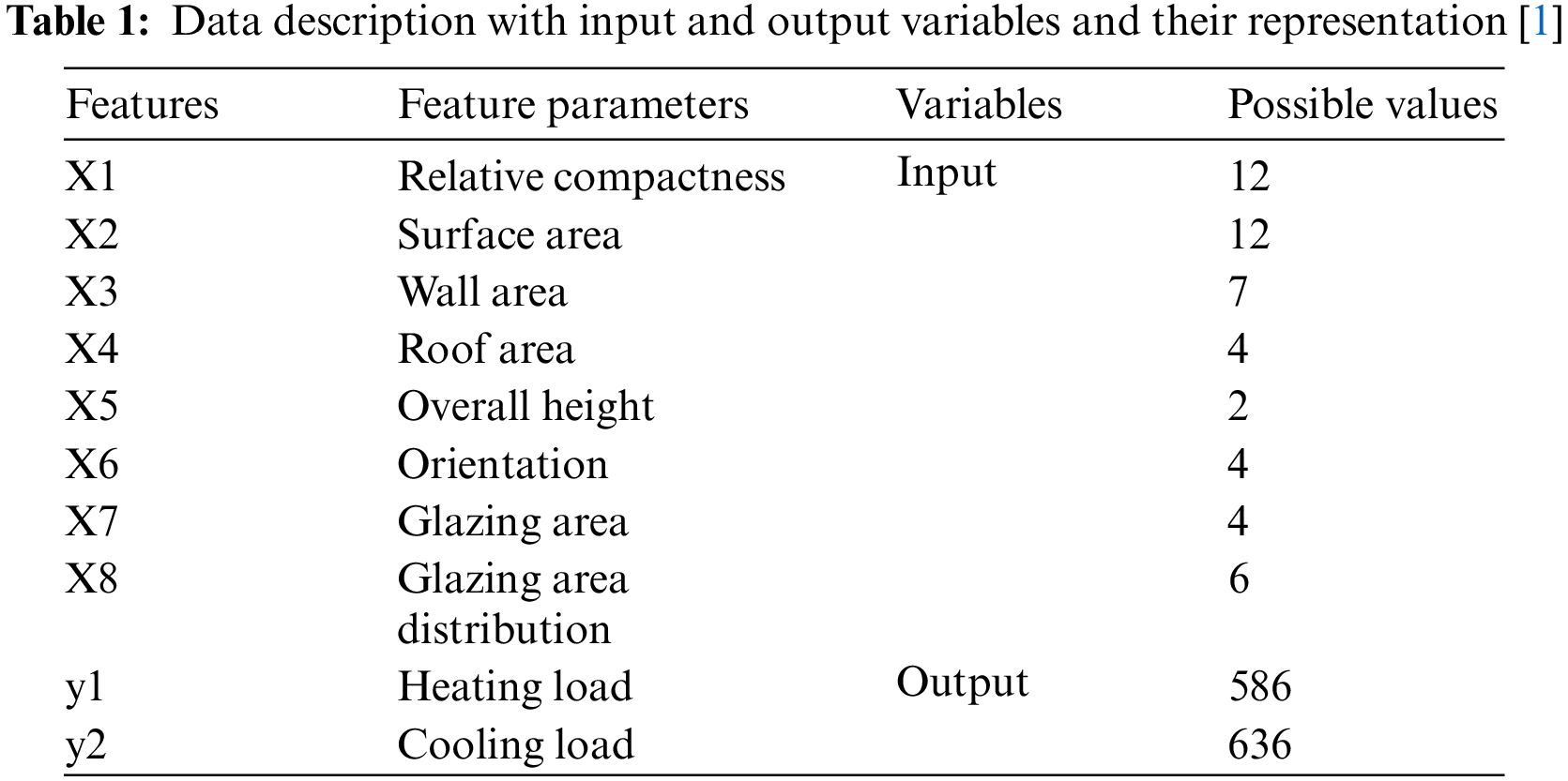
The dataset is based on the energy analysis performed using 12 building shapes simulated in Ecotect and is publicly available at [1]. The dataset comprises parameters that determine the CL and HL of the generated shapes and includes the relative compactness, glazing area, glazing area distribution, wall area, surface area, roof area, overall height, and orientation. A total of 768 shapes were simulated using various settings as functions of the characteristic. Thus, the dataset uses eight features to predict two real-valued responses (HL and CL). This work considers the prediction task to be a multiple-input and multiple-output regression problem. When the response is rounded to the nearest integer, the dataset can be used for a multiclass classification problem. The proposed model was trained and validated with 600 and 168 data samples. Table 1 presents the dataset descriptions and attributes.

2.1 One-Dimensional Convolutional Neural Network Prediction of Heating and Cooling Load

As discussed in the introduction, most studies treat the problem of energy prediction as a univariate prediction problem. This paper aims to design a multivariate 1D CNN model for predicting building energy load, HL and CL. The proposed architecture for this problem is a multi-input and multi-output architecture that takes eight parameters (i.e., building characteristics) as input and predicts the building HL and CL as outputs (Fig. 1). The building characteristics contain attributes defined as the shape of buildings on which HL and CL depend. Section 2.2 discusses the 1D models in detail.

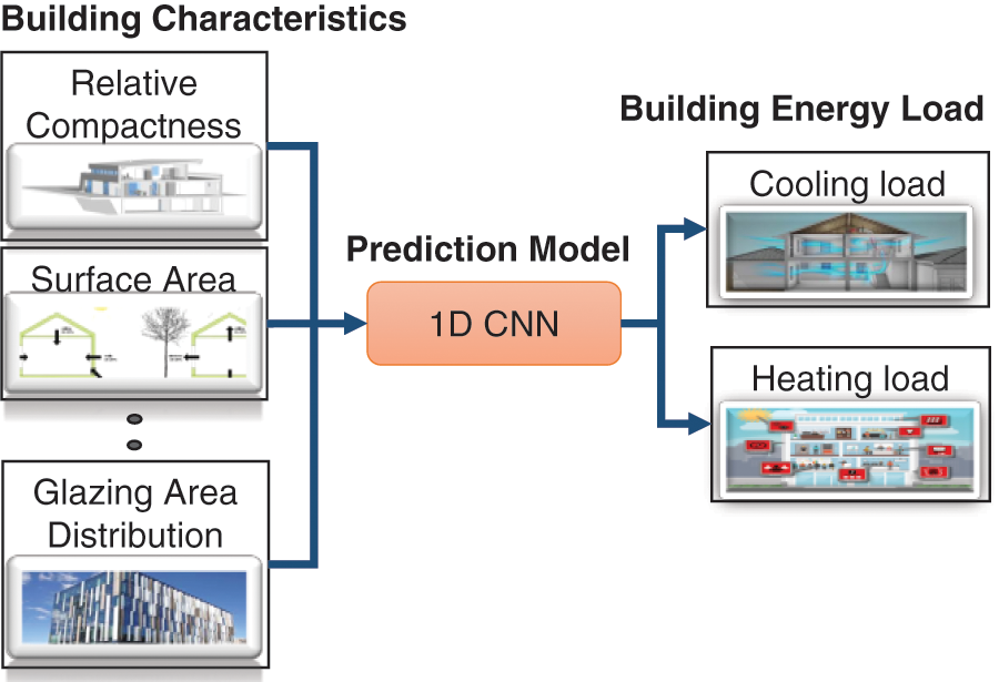
Figure 1: Cooling and heating load prediction block diagram

2.2 Multivariate Energy Load Prediction with the Convolutional Neural Network

We proposed a 1D multivariate CNN for predicting the HL and CL in this work. A 1D CNN has convolutional and pooling layers that operate over a 1D sequence of input data. The model learns a function that maps the data attributes as input that predicts two real-valued responses, HL and CL, as output. The convolutional layer extracts features, and the dense fully connected layer interprets the features. The flattened layer reduces the feature maps to a single 1D vector. In the implementation, the pooling layer is not applied because 1D data are unaffected by excessive parameters, and its use has been questioned in recent studies [35]. The proposed architecture consists of a convolutional layer with 64 neurons, a flattened layer, a dense layer of 50 neurons, and a dense output layer of two neurons (Fig. 2). The architecture was derived through experiments to create a light model. The data were first normalized in the range of −1 to 1 and then reshaped into a 3D structure acceptable by the CNN where each row and column are the time steps and separate time series, respectively. Hyperparameters were determined by the experiment, as subsequently presented.

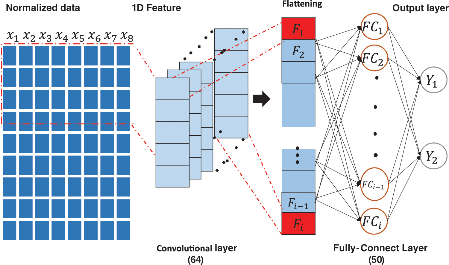
Figure 2: 1D CNN architecture for multivariate energy load prediction

Prediction can be configured in two main ways: directly or iteratively [35]. In direct prediction, the model produces the desired output at once. Hence, the output layer consists of neurons equal to the intended prediction horizon. For iterative prediction, the network predicts only a one-time step. In this study, we employed an iterative method using one time step consisting of eight inputs and two outputs. The model is evaluated using 10-fold cross-validation.

With the building representation as the model input, the input vector can describe as follows:

X →={X1, X2, X3, X4, X5, X6, X7, X8}(1)

where X → represents the characteristics of the building for time step, t. The model predicts the CL and HL for a given time t. The output vector is expressed as follows:

Y→={Y1, Y2}.(2)

The typical CNN model is used to estimate a function f  defined by Y→=f(X →; θ), where X → and Y→ denote the input and output of the CNN, respectively [36]. The network parameter (weights) θ of the CNN parameterize the estimated function f^(X; θ). The network parameters were estimated during the training phase by minimizing the loss function l(θ):

θt=argminθ l(θ).(3)

Optimization algorithms are crucial hyperparameters for deep learning because they determine the training speed and model performance. There is no theory guide when comparing optimizers, but the popular first-order optimizers form a natural inclusion hierarchy. In general, the first partial derivative of the loss function is given as ∇l(θ), with l representing the loss computed over the dataset. For instance, in the first-order iterative method, the optimizer determines a point that minimizes l by constructing a sequence θt based on l(θ) and ∇l(θ) using an update rule ℳ, which employs the iteration history, Ht={θs, ∇l(θ)s, l(θ)s}s=0t and the hyperparameter, ϕt, to determine the next θt+1:

θt+1=ℳ(Ht,ϕt).(4)

The main difference between optimizers depends on the selection update for ℳ and ϕ. As the model effectiveness depends on the right optimizers for a problem, we conducted an extensive experiment to determine the optimal optimizer for this problem. The considered optimizers include adaptive moment estimation (Adam), Adaptive Gradient Algorithm (AdaGrad), Stochastic gradient descent (SGD), and Root Mean Squared Propagation (RMSprop).

Furthermore, convolution, activation, and pooling are performed at each CNN layer. The convolutional operation is defined for a 2D input I by

τ(i,j)=(X →⊗F)(i,j)=∑m,nX →(i+m, j+n)F(m,n),(5)

where I represents input data, F∈Rm×n indicates the filters or kernels, and ⊗ denotes the convolutional operation. In addition, τ(x,y) is the value of feature map τ(i,j) computed at the location (i,j). The convolutional operation is performed at the location (i,j), and the filter F shifts over to the next location with the amount of shift controlled by the stride. The convolutional operation is followed by a nonlinear activation function (AF, e.g., rectified linear units [ReLU]) and nonlinear downsampling (pooling). The pooling substitutes the input  X →=(i,j) at location (i,j) with ψ(N(i,j)), where N(x,y) denotes the neighborhood of (i,j) and ψ is a pooling function with summary statistics, such as max-pooling, applying the operation max(a,b)=a, if a>b.

An AF is used to compute the weighted sum of inputs and biases on which a neuron depends to determine whether to fire. The AF, which can either be linear or nonlinear depending on the function it represents, controls the outputs of neural networks across domains, such as prediction, object recognition, and classification [37–41]. The proper choice of AF for a given application can significantly improve the results. This study investigates the performance of various AF (see Section 3.). The backgrounds of a few investigated AFs are as follows.

2.2.1 Sigmoid Function

The sigmoid AF is a nonlinear, bounded differentiable function used at the output layer of the deep learning architecture to predict probabilities based on the output. It has been applied to various problems, such as binary classification problems and logistic regression tasks [41]. It has several variants, but the general form is given as follows:

f(τ)=(1(1+e−τ)).(6)

2.2.2 Rectified Linear Unit Function

The ReLU is a linear function that addresses the vanishing gradient problem by rectifying input values less than zero to zero through a thresholding operation. It has been applied within hidden deep learning layers and offers a faster computation than other AFs, such as the sigmoid and tanh. It is given as follows:

f(τ)={τi if τi≥00, if τi< 0.(7)

2.2.3 Exponential Linear Unit Function

The exponential linear unit (ELU) function is an alternative to ReLU, which eliminates the vanishing gradient problem and improves learning speed using the positive value identity and allowing negative values. It reduces computational complexity by pushing the mean activation unit closer to zero. It is defined as follows:

f(τ)={τ,             if τ>0αeτ−1, if τ≤ 0,(8)

where α is the hyperparameter that controls the saturation point for negative net inputs.

2.2.4 Scaled Exponential Linear Units

The scaled ELU (SELU) function is a variant of ELU that enforces self-normalizing properties when propagated through multiple layers during training by converging to a zero mean and unit variance, enabling strong regularization for robust feature learning. It is given as follows:

f(τ)={τ,             if τ>0αeτ−α, if τ≤ 0,(9)

where α is the saturation point hyperparameter for negative net inputs.

2.2.5 Performance Evaluation Metric

The performance metric considered for the investigation is the MSE, which measures the average of the squares of the errors (i.e., the average squared difference between the predicted and actual values). Mathematically, MSE is defined as follows:

MSE=1n∑1n(y−y^)2,(10)

where y denotes the true independent variable, and y^ represents the predicted independent variable.

3  Results and Discussion

In this section, the experiments were conducted to rigorously investigate the optimal hyperparameter setup for the multivariate prediction of CL and HL of a building based on shape. The investigated hyperparameters include epochs, AFs, and optimizers. The experiments were repeated several times to address the random initialization of the network parameters that may lead to different results each time the network is trained. The experiments were implemented with the Keras library using a Windows 10 desktop computer with a CORE i7 Intel processor, GTX 760 graphics card, and 8 GB of RAM.

For preprocessing, the shape of input X in the proposed model is reshaped into three dimensions, including the number of samples (600 for training), number of time steps (1), and number of parallel time series or features (8). The shape of the output, Y→, is 2D: the number of samples (600) and number of variables per sample to be predicted (two). Therefore, the normalized data are reshaped into 3D and 2D for each sample input, X, and output, y, for each sample. The entire procedure is repeated using a batch size of four until all data points are predicted.

First, we explored the statistical properties of the variables, which is typically achieved by plotting the probability densities to summarize each variable succinctly for visualization. As observed from the probability distribution in Fig. 3, no variable has a normal distribution, so this cannot be easily solved using classical models. The “orientation” and “overall height” features have an even distribution, while most features are positively skewed, as illustrated in Fig. 3a. For the dependent variables, the samples fall between 10 and 20 with a positive skew, as depicted in Fig. 3b. These observations were also made in [1] and [42]. Moreover, the correlation matrix in Fig. 3c reveals that fewer features can be used to predict the energy loads. However, we investigated how the 1D CNN can learn with the full features in this work.

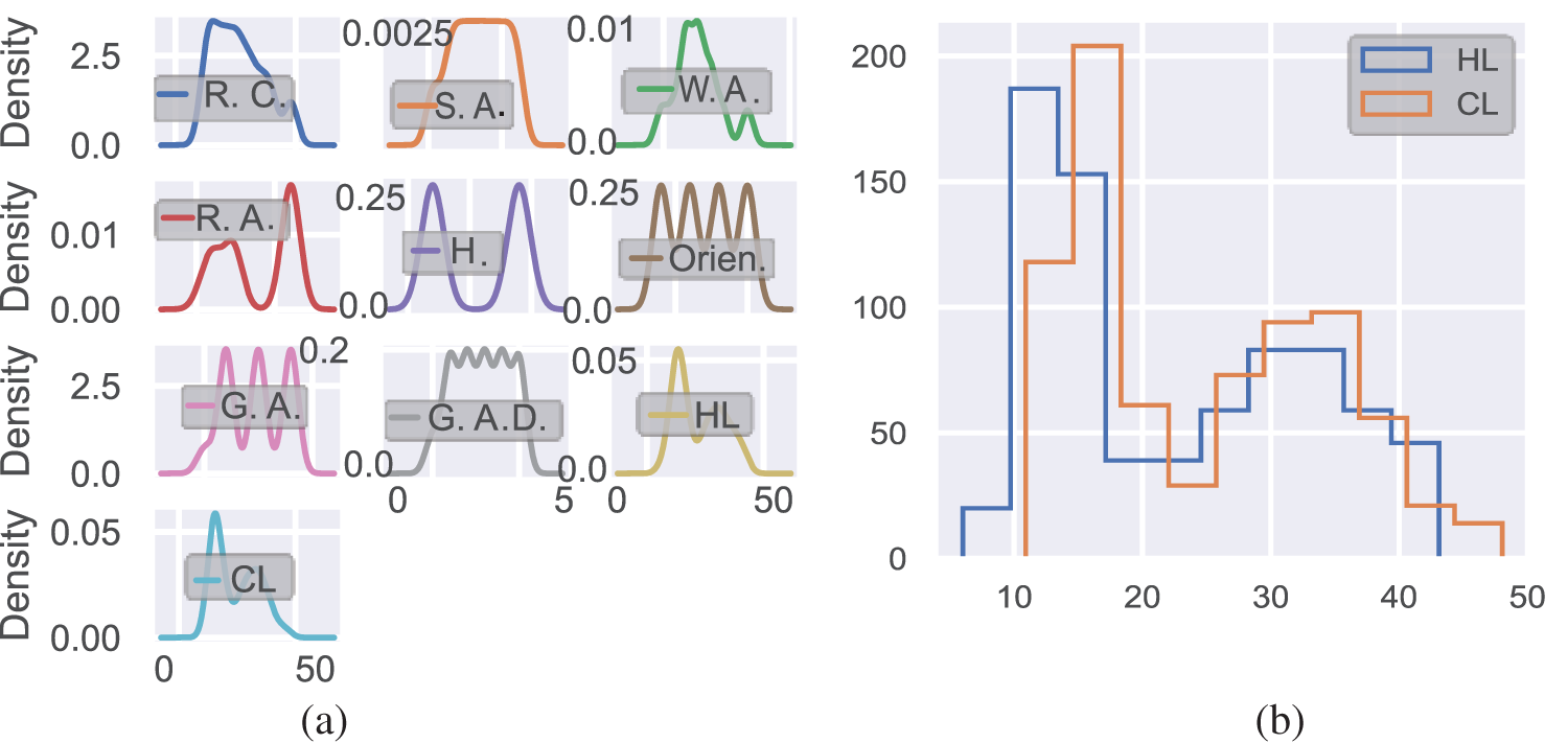
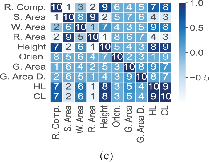
Figure 3: Data visualization analysis: (a) positively skewed probability distribution, (b) histogram positively skewed distribution of dependent variables, and (c) correlation matrix

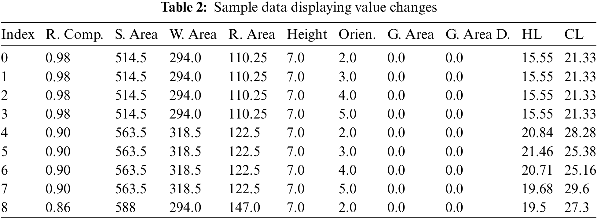
3.1 Determination of the Model Optimal Hyperparameters

This section investigates the hyperparameters of the 1D CNN for the prediction of HL and CL. The default model consists of one convolutional layer with 64 neurons, a flattened layer, a dense layer of 50 neurons, and a dense output layer of two neurons. As illustrated in the sample data in Table 2, the values of the first four features were changed after every four samples. Based on this assumption, we selected a batch size of four, which would afford the model a better understanding of the feature patterns and the corresponding dependent variables, HL and CL.

The first considered hyperparameter was the epoch, and the experimental setup is presented in Fig. 4. Five epochs (100, 200, 300, 400, and 500) were investigated to obtain the optimal value for the best generalization. Each epoch was experimented with and evaluated using k-fold cross-validation to address bias caused by randomness in choosing testing cases. As depicted in Fig. 5, epochs of 300 and 400 performed the best with the MSE at approximately 0.0038 and 0.0075 for the mean and 0.0036 and 0.0067 for the standard deviation. Epochs of 400 provided a better MSE compared to epochs of 300. However, because we used various AFs and optimization methods, we conservatively performed 300 iterations for the rest of the experiments.

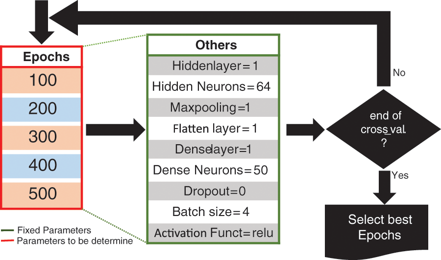
Figure 4: Epoch selection process

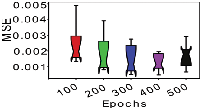
Figure 5: Epoch performance using k-fold

Next, we investigated nine AFs and four optimizer hyperparameters. The AFs include ELU, exponential, ReLU, sigmoid, softmax, softplus, softsign, and hyperbolic tangent (tanh). Each AF was experimented with by applying each optimization algorithm using the fixed hyperparameters five times, as depicted in Fig. 6. Thus, a total of about 180 experiments was conducted to select the best combination of AF and optimizer.

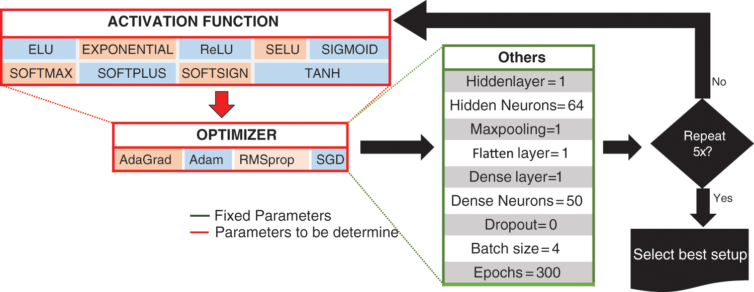
Figure 6: Activation function selection process applying various optimizer algorithms

Fig. 7a illustrates the ELU performance with various optimizers. In training, Adam and RMSprop demonstrated the best performance of less than 0.005 for the MSE, but the validation phase for Adam displayed overfitting at around 60 epochs. In contrast, the validation performance of RMSprop is the best at about 0.01 for the MSE, although it experiences outfitting beyond the 75 epochs with regular spikes between 0.02 and 0.03 for the MSE. Therefore, based on this result, more experimentation is needed to use Adam and the SGD to obtain the best performance with the optimal optimizer when using the ELU AF. On the other hand, the SELU AF generalizes to less than 0.01 for the MSE for the RMSprop and Adam optimizers in the learning phase (Fig. 7b). For the validation, Adam and RMSprop are below 0.01 for the MSE at 75 epochs but experience bumps and spikes beyond 75 epochs. Furthermore, the ReLU with Adam and RMSprop performed best for the MSE with a training and validation recording of less than 0.005 and 0.01 for the MSE, respectively, at about 25 epochs (Fig. 7c).

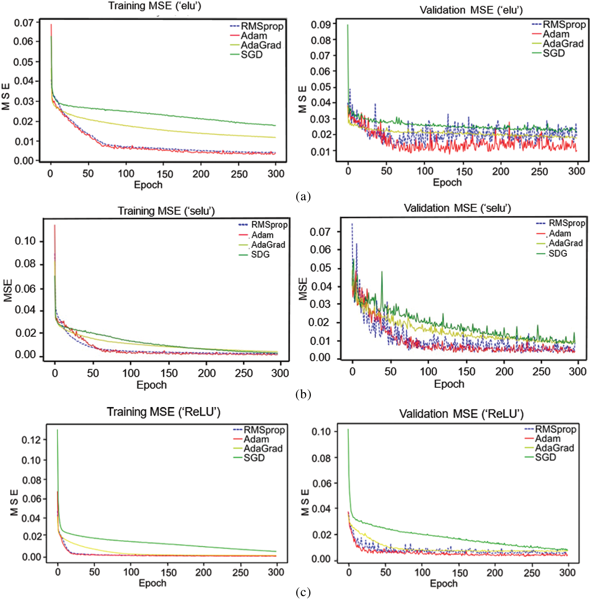
Figure 7: Activation function performance with various optimizers: (a) ELU, (b) SELU, and (c) ReLU

Similarly, the rest of the AFs were investigated. The exponential AF was generalized to about zero for the MSE for all optimizers in the learning phase. For the validation, Adam and RMSprop performed best for an MSE of about 0.01 at around 150 epochs. Thus, the exponential AF with Adam or RMSprop is the best option for fast application. In addition, the training performance for the rest of the AFs (sigmoid, softmax, softplus, softsign, and tanh) exhibited the best performance in combination with Adam. Likewise, their validation performance was the best, except for tanh, in which the Adam optimizer experienced overfitting. Furthermore, the configuration of softmax with SGD resulted in the poorest performance compared to any considered configuration. Thus, based on the results, the ReLU AF and Adam optimizer are adequate for predicting the CL and HL.

3.2 Model Prediction Performance

The optimal training epoch and optimizer were 300 and Adam, respectively. Next, we evaluated the performance of the AFs using the optimal epoch and optimizer performance evaluation using a 10-fold cross-validation index. Except for the softmax AF with about 10 for the MSE, the rest of the AFs generalize with an MSE of less than 4 (Fig. 8). The best result was recorded using the ReLU AF with an MSE of about 0.003828. The worst performance was the model using the softmax AF, as it is theoretically for classification problems. In this study, the AF, optimizer, and number of epochs that achieved optimal performance were ReLU, Adam, and 300, respectively.

Figure 8: Performance evaluation of various activation functions using 10-fold cross-validation

Fig. 10 presents the comparison plot between the real and predicted building energy load using the proposed model for the training data. The predicted 1D CNN model fits the trend in the observed energy load (i.e., HL and CL data). The model observed no significant deviation in the prediction of HL and CL. Fig. 10a illustrates the real and predicted values for both the HL and CL on the same axis, but for clarity, we split the plot into HL and CL, as depicted in Figs. 9a and 9b, respectively.

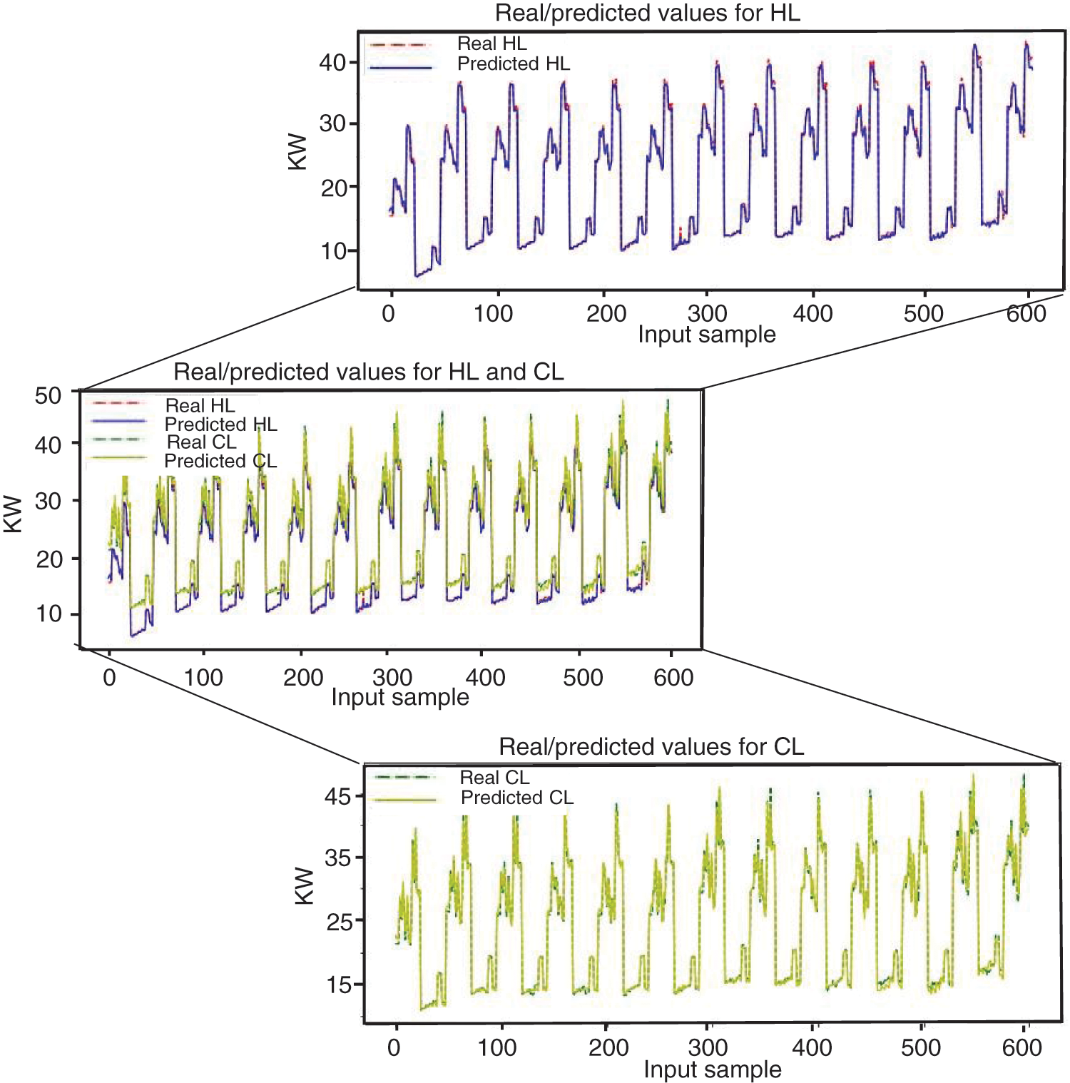
Figure 9: Multivariate model on training data, actual and prediction: (a) HL and CL, (b) CL, and (c) HL

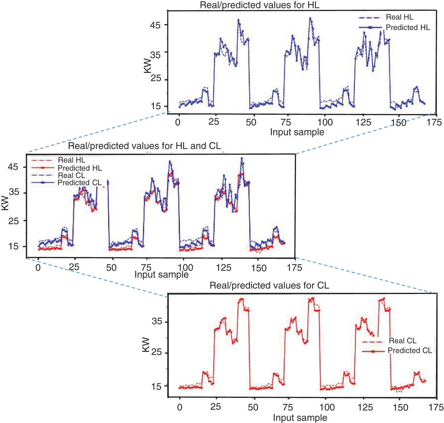
Figure 10: Multivariate model on testing data actual and prediction: (a) HL and CL, (b) CL, and (c) HL

Similarly, using testing data, Fig. 10 compares the real and predicted building energy load with the proposed model. The prediction result demonstrates that the proposed model fits the observed data trend. As indicated in Figs. 11a and 11b, no significant underprediction was observed in the testing data. The results reflect the low MSE recorded by this model.

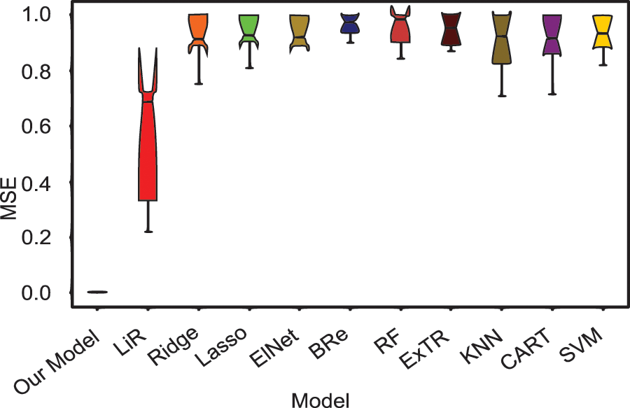
Figure 11: Performance evaluation of the proposed vs. classical models using 10-fold cross-validation

3.3 Model Evaluation Against Other Algorithms

The performance of various classical models was compared against the proposed model. The classical models compared with the proposed model were linear regression (LiR), Ridge, Lasso, ElasticNet (ElNet), extra tree regressor (ExtTR), K-nearest neighbors (KNN), classification and regression tree (CART), and support vector machine (SVM). As presented in Fig. 11, the proposed model outperformed all other models, with LiR ranking second with a mean performance of about 0.7 for the MSE.

Furthermore, the proposed model exhibited excellent results in terms of performance compared to other related models using the same dataset. The proposed model performance can be improved using 400 epochs, as discussed in Section 3.1. Thus, we considered the 400 and 300 epochs models against related models. The algorithms in related research include SVR with the artificial neural network [2], SVR [2], iteratively reweighted least squares (IRLS) [2], RF [1], GBRT [12], and genetic programming [11]. Although predictive algorithms are based on a univariate prediction problem, the proposed model displays a comparative advantage over the related models (Fig. 12). The proposed model best performed with 0.003553 for the MSE. In contrast, the GBRT, SVR, and IRLS performed second, third, and worst with MSEs of 0.10, 0.12, and 11.46, respectively. The proposed model significantly reduces the MSE by about 28 times the best-performing model, GBRT [12].

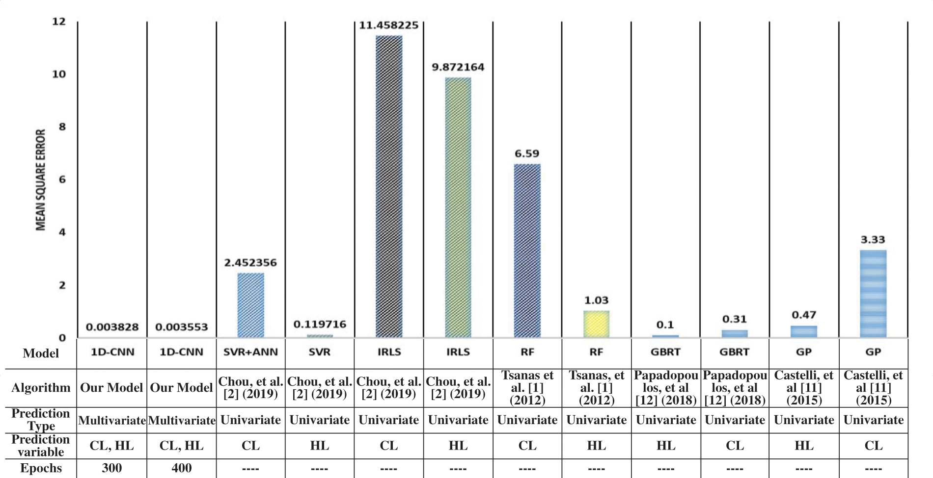
Figure 12: Performance evaluation of the proposed model against related studies

4  Conclusion

In this paper, we investigated using a 1D CNN model for multivariate prediction of building energy performance. The detailed experimental results were presented for various AFs, optimizers, and optimal epochs for predicting HL and CL. According to the experimental results, the model we presented best predicted HL and CL using the ReLU AF, Adam optimizer, and 400 training epochs. Furthermore, the proposed model is better than the presented existing models, resulting in an MSE of about 0.0035, about 28 times better than the best-performing model, GBRT. It also saves computational time while training two univariate models for HL and CL. Although the proposed model is built based on simulation data that only consider building characteristics, using multivariate prediction with 1D CNN may offer more flexibility and better performance for the effective prediction of building energy performance. Future research can consider other dynamic external factors, such as weather, to efficiently design robust and applicable models for building energy load prediction, considering the environmental factors and geographic location of the building.

Funding Statement: This work was supported in part by the Institute of Information and Communications Technology Planning and Evaluation (IITP) Grant by the Korean Government Ministry of Science and ICT (MSIT; Artificial Intelligence Innovation Hub) under Grant 2021-0-02068; and in part by the National Research Foundation of Korea (NRF) Grant by the Korean Government (MSIT) under Grant NRF-2021R1I1A3060565.

Conflicts of Interest: The authors declare that they have no conflicts of interest to report regarding the present study.

References

1. A. Tsanas and A. Xifara, “Accurate quantitative estimation of energy performance of residential buildings using statistical machine learning tools,” Energy and Buildings, vol. 49, pp. 560–567, 2012. [Google Scholar]

2. J. -S. Chou and D. -K. Bui, “Modeling heating and cooling loads by artificial intelligence for energy-efficient building design,” Energy and Buildings, vol. 82, pp. 437–446, 2014. [Google Scholar]

3. A. Micheal, F. Abiodun, O. Mikail and A. Ibrahim, “Human body temperature based air conditioning control system,” International Journal of Engineering Research & Technology (IJERT), vol. 3, no. 5, pp. 2474–2479, 2014. [Google Scholar]

4. S. Fathi, R. Srinivasan, A. Fenner and S. Fathi, “Machine learning applications in urban building energy performance forecasting: A systematic review,” Renewable and Sustainable Energy Reviews, vol. 133, pp. 110287, 2020. [Google Scholar]

5. K. U. Ahn, H. S. Shin and C. S. Park, “Energy analysis of 4625 office buildings in South Korea,” Energies, vol. 12, no. 6, pp. 1114, 2019. [Google Scholar]

6. S. Gunasingh, N. Wang, D. Ahl and S. Schuetter, “Climate resilience and the design of smart buildings,” in Smart Cities: Foundations, Principles, and Applications, 1st ed., River Street, Hoboken, NJ 07030, USA: John Wiley & Sons, Inc., pp. 667–641, 2017. [Google Scholar]

7. A. Yezioro, B. Dong and F. Leite, “An applied artificial intelligence approach towards assessing building performance simulation tools,” Energy and Buildings, vol. 40, no. 4, pp. 612–620, 2008. [Google Scholar]

8. T. Hong, P. Pinson, Y. Wang, R. Weron, D. Yang et al., “Energy forecasting: A review and outlook,” IEEE Open Access Journal of Power and Energy, vol. 7, pp. 376–388, 2020. [Google Scholar]

9. I. Aliyu, U. Kamoliddin, S. J. Seong, S. Cen, Y. Zhao et al., “CNN-LSTM for smart grid energy consumption prediction,” in Presented at the 2021 Int. Conf. on Convergence Content (ICCC), Jeju, South Korea, pp. 29–30, 2021. [Google Scholar]

10. H. Borchani, G. Varando, C. Bielza and P. Larrañaga, “A survey on multi-output regression,” Wiley Interdisciplinary Reviews: Data Mining and Knowledge Discovery, vol. 5, no. 5, pp. 216–233, 2015. [Google Scholar]

11. M. Castelli, L. Trujillo, L. Vanneschi and A. Popovič, “Prediction of energy performance of residential buildings: A genetic programming approach,” Energy and Buildings, vol. 102, pp. 67–74, 2015. [Google Scholar]

12. S. Papadopoulos, E. Azar, W. -L. Woon and C. E. Kontokosta, “Evaluation of tree-based ensemble learning algorithms for building energy performance estimation,” Journal of Building Performance Simulation, vol. 11, no. 3, pp. 322–332, 2018. [Google Scholar]

13. S. S. Roy, R. Roy and V. E. Balas, “Estimating heating load in buildings using multivariate adaptive regression splines, extreme learning machine, a hybrid model of MARS and ELM,” Renewable and Sustainable Energy Reviews, vol. 82, pp. 4256–4268, 2018. [Google Scholar]

14. I. Bilous, V. Deshko and I. Sukhodub, “Parametric analysis of external and internal factors influence on building energy performance using non-linear multivariate regression models,” Journal of Building Engineering, vol. 20, pp. 327–336, 2018. [Google Scholar]

15. K. Amarasinghe, D. L. Marino and M. Manic, “Deep neural networks for energy load forecasting,” in 2017 IEEE 26th Int. Symp. on Industrial Electronics (ISIE), Edinburgh, UK, IEEE, pp. 1483–1488, 2017. [Google Scholar]

16. R. E. Brown, T. Walter, L. N. Dunn, C. Y. Custodio, P. A. Mathew et al., “Getting real with energy data: Using the buildings performance database to support data-driven analyses and decision-making,” in Proc. of the ACEEE Summer Study on Energy Efficiency in Buildings, California, CA, USA, pp. 11–49, 2014. [Google Scholar]

17. S. Mishra, C. Bordin, K. Taharaguchi and I. Palu, “Comparison of deep learning models for multivariate prediction of time series wind power generation and temperature,” Energy Reports, vol. 6, pp. 273–286, 2020. [Google Scholar]

18. S. Cavalli and M. Amoretti, “CNN-Based multivariate data analysis for bitcoin trend prediction,” Applied Soft Computing, vol. 101, pp. 107065, 2021. [Google Scholar]

19. X. Dong, M. Guo and S. Wang, “Advanced prediction of the sinking speed of open caissons based on the spatial-temporal characteristics of multivariate structural stress data,” Applied Ocean Research, vol. 127, pp. 103330, 2022. [Google Scholar]

20. X. Xie, B. Wang, T. Wan and W. Tang, “Multivariate abnormal detection for industrial control systems using 1D CNN and GRU,” IEEE Access, vol. 8, pp. 88348–88359, 2020. [Google Scholar]

21. R. Assaf, I. Giurgiu, F. Bagehorn and A. Schumann, “Mtex-cnn: Multivariate time series explanations for predictions with convolutional neural networks,” in 2019 IEEE Int. Conf. on Data Mining (ICDM), Beijing, China, pp. 952–957, 2019. [Google Scholar]

22. B. S. Shawel, E. Mare, T. T. Debella, S. Pollin and D. H. Woldegebreal, “A multivariate approach for spatiotemporal mobile data traffic prediction,” Engineering Proceedings, vol. 18, no. 1, pp. 10, 2022. [Google Scholar]

23. C. W. Hong, K. Lee, M. -S. Ko, J. -K. Kim, K. Oh et al., “Multivariate time series forecasting for remaining useful life of turbofan engine using deep-stacked neural network and correlation analysis,” in 2020 IEEE Int. Conf. on Big Data and Smart Computing (BigComp), IEEE, Busan, Korea (Southpp. 63–70, 2020. [Google Scholar]

24. D. Hussain, T. Hussain, A. A. Khan, S. A. A. Naqvi and A. Jamil, “A deep learning approach for hydrological time-series prediction: A case study of Gilgit river basin,” Earth Science Informatics, vol. 13, no. 3, pp. 915–927, 2020. [Google Scholar]

25. S. Kiranyaz, O. Avci, O. Abdeljaber, T. Ince, M. Gabbouj et al., “1D convolutional neural networks and applications: A survey,” Mechanical Systems and Signal Processing, vol. 151, pp. 107398, 2021. [Google Scholar]

26. W. Tang, G. Long, L. Liu, T. Zhou, M. Blumenstein et al., “Omni-scale CNNs: A simple and effective kernel size configuration for time series classification,” in Int. Conf. on Learning Representations, online, pp. 1–17, 2021. [Google Scholar]

27. S. Kiranyaz, T. Ince, R. Hamila and M. Gabbouj, “Convolutional neural networks for patient-specific ECG classification,” in 37th Annual Int. Conf. of the IEEE Engineering in Medicine and Biology Society (EMBC), Milan, Italy, pp. 2608–2611, 2015. [Google Scholar]

28. S. Kiranyaz, T. Ince and M. Gabbouj, “Real-time patient-specific ECG classification by 1-D convolutional neural networks,” IEEE Transactions on Biomedical Engineering, vol. 63, no. 3, pp. 664–675, 2015. [Google Scholar] [PubMed]

29. O. Abdeljaber, O. Avci, S. Kiranyaz, M. Gabbouj and D. J. Inman, “Real-time vibration-based structural damage detection using one-dimensional convolutional neural networks,” Journal of Sound and Vibration, vol. 388, pp. 154–170, 2017. [Google Scholar]

30. O. Abdeljaber, A. Younis, O. Avci, N. Catbas, M. Gul et al., “Dynamic testing of a laboratory stadium structure,” in Geotechnical and Structural Engineering Congress 2016, Phoenix, Arizona, pp. 1719–1728, 2016. [Google Scholar]

31. O. Abdeljaber, O. Avci, M. Kiranyaz, B. Boashash, H. Sodano et al., “1-D CNNs for structural damage detection: Verification on a structural health monitoring benchmark data,” Neurocomputing, vol. 275, pp. 1308–1317, 2018. [Google Scholar]

32. T. Ince, S. Kiranyaz, L. Eren, M. Askar and M. Gabbouj, “Real-time motor fault detection by 1-D convolutional neural networks,” IEEE Transactions on Industrial Electronics, vol. 63, no. 11, pp. 7067–7075, 2016. [Google Scholar]

33. L. Eren, T. Ince and S. Kiranyaz, “A generic intelligent bearing fault diagnosis system using compact adaptive 1D CNN classifier,” Journal of Signal Processing Systems, vol. 91, no. 2, pp. 179–189, 2019. [Google Scholar]

34. L. Eren, “Bearing fault detection by one-dimensional convolutional neural networks,” Mathematical Problems in Engineering, vol. 2017, pp. 1–9, 2017. [Google Scholar]

35. C. Lang, F. Steinborn, O. Steffens and E. W. Lang, “Electricity load forecasting–An evaluation of simple 1D-CNN network structures,” arXiv preprint arXiv:1911.11536, 2019. [Google Scholar]

36. S. Liu, M. Ozay, T. Okatani, H. Xu, K. Sun et al., “A vision based system for underwater docking,” arXiv preprint arXiv:1712.04138, 2017. [Google Scholar]

37. S. S. Md Noor, K. Michael, S. Marshall and J. Ren, “Hyperspectral image enhancement and mixture deep-learning classification of corneal epithelium injuries,” Sensors, vol. 17, no. 11, pp. 2644, 2017. [Google Scholar]

38. R. Hu, P. Dollár, K. He, T. Darrell and R. Girshick, “Learning to segment every thing,” in Proc. of the IEEE Conf. on Computer Vision and Pattern Recognition, Salt Lake City, UT, USA, pp. 4233–4241, 2018. [Google Scholar]

39. Y. Liu and J. Zhang, “Deep learning in machine translation,” in Deep Learning in Natural Language Processing, Singapore: Springer, pp. 147–183, 2018. [Google Scholar]

40. M. A. Adegboye, A. M. Aibinu, J. G. Kolo, I. Aliyu, T. A. Folorunso et al., “Incorporating intelligence in fish feeding system for dispensing feed based on fish feeding intensity,” IEEE Access, vol. 8, pp. 91948–91960, 2020. [Google Scholar]

41. C. Nwankpa, W. Ijomah, A. Gachagan and S. Marshall, “Activation functions: Comparison of trends in practice and research for deep learning,” arXiv preprint arXiv:1811.03378, 2018. [Google Scholar]

42. A. D. Akogo. “Analyzing and modelling energy efficiency,” (accessed May, 2022). https://www.kaggle.com/elikplim/analysing-and-modelling-energy-efficiency [Google Scholar]