
 Submit a Paper
 Propose a Special lssue
 Open Access
ARTICLE

Bi-LSTM-Based Deep Stacked Sequence-to-Sequence Autoencoder for Forecasting Solar Irradiation and Wind Speed
1 Department of Electrical and Computer Engineering, COMSATS University Islamabad, Lahore Campus, 45550, Pakistan
2 School of Engineering and Technology, National Textile University, Faisalabad, 37610, Pakistan
3 Department of Electrical Engineering, Information Technology University, Lahore, 54000, Pakistan
4 Department of Electrical Engineering, GC University, Faisalabad, 38000, Pakistan
5 Faculty of Mechanical and Industrial Engineering, Warsaw University of Technology, 02-524, Warsaw, Poland
* Corresponding Author: Krzysztof Ejsmont. Email:
Computers, Materials & Continua 2023, 75(3), 6375-6393. https://doi.org/10.32604/cmc.2023.038564
Received 19 December 2022; Accepted 08 February 2023; Issue published 29 April 2023
 View Full Text
 Download PDF
Abstract
Wind and solar energy are two popular forms of renewable energy used in microgrids and facilitating the transition towards net-zero carbon emissions by 2050. However, they are exceedingly unpredictable since they rely highly on weather and atmospheric conditions. In microgrids, smart energy management systems, such as integrated demand response programs, are permanently established on a step-ahead basis, which means that accurate forecasting of wind speed and solar irradiance intervals is becoming increasingly crucial to the optimal operation and planning of microgrids. With this in mind, a novel “bidirectional long short-term memory network” (Bi-LSTM)-based, deep stacked, sequence-to-sequence autoencoder (S2SAE) forecasting model for predicting short-term solar irradiation and wind speed was developed and evaluated in MATLAB. To create a deep stacked S2SAE prediction model, a deep Bi-LSTM-based encoder and decoder are stacked on top of one another to reduce the dimension of the input sequence, extract its features, and then reconstruct it to produce the forecasts. Hyperparameters of the proposed deep stacked S2SAE forecasting model were optimized using the Bayesian optimization algorithm. Moreover, the forecasting performance of the proposed Bi-LSTM-based deep stacked S2SAE model was compared to three other deep, and shallow stacked S2SAEs, i.e., the LSTM-based deep stacked S2SAE model, gated recurrent unit-based deep stacked S2SAE model, and Bi-LSTM-based shallow stacked S2SAE model. All these models were also optimized and modeled in MATLAB. The results simulated based on actual data confirmed that the proposed model outperformed the alternatives by achieving an accuracy of up to 99.7%, which evidenced the high reliability of the proposed forecasting.Keywords
Index of Notation and Abbreviations
| ANFIS | Adaptive network-based fuzzy inference system |
| ANN | Artificial neural network |
| ARIMA | Autoregressive integrated moving average model |
| ARMA | Autoregressive moving average model |
| Bi-LSTM | Bi-directional long short-term memory networks |
| BP-NN | Backpropagation neural network |
| CART | Classification and regression tree |
| CNN | Convolutional neural networks |
| DBN | Deep brief networks |
| DL | Deep learning |
| ELM | Extreme learning machine |
| GBDT | Gradient boosting decision tree |
| GHI | Global horizontal irradiance |
| GPR | Gaussian process regression |
| GR-NN | Generalized regression neural network |
| GRU | Gated recurrent unit |
| LSSVM | Least-squares support vector machine |
| LSTM | Long short-term memory networks |
| M5Tree | Model five tree |
| MAPE | Mean absolute percentage error |
| MLP-NN | Multi-layer perception neural network |
| RBF-NN | Radials basis function neural network |
| RMSE | Root mean square error |
| RNN | Recurrent neural networks |
| S2SAE | Sequence-to-sequence autoencoder |
| SAE | Stacked autoencoder |
| SVM | Support vector machine |
| Backward hidden state | |
| Forward hidden state | |
| Input | |
| b | Bias term |
| Hidden representation | |
| h[t] | Cell’s output |
| s[t] | Cell state |
| tanh | Hyperbolic tangent activation function |
| W | Weight matrix |
| σ | Sigmoid activation function |
| Input of forget gate | |
| ig | Input of input gate |
| og | Input of output gate |
| Activation function | |
| Activation function | |
| u | Update signal |
With the rapid development of smart grids, microgrids have been garnering increasing interest as a unique method of power delivery. A microgrid is a small-scale self-sustained intelligent power system designed to deliver electricity to regional and local users, e.g., businesses. It may function in an islanded state during grid disruptions or can be grid-connected. Notably, such solutions have the potential to minimize energy delivery costs, increase load-point dependability, improve power quality, reduce emissions from power generation, manage investment costs in power transmission, and also improve the susceptibility of large-scale power systems [1]. However, traditional microgrids still face a significant challenge posed by the erratic nature of renewable energy sources. Industry 4.0 aims to encourage the integration of industrial multi-energy microgrids and the application of internet technologies to renewable energy through smart energy management systems such as demand-response programs. Renewable energy sources, including water [2–4], waste, sunlight, wind, and heat from the Earth, are naturally replenished and produce negligible amounts of greenhouse gases and air pollution. Globally, the US Department of Energy has defined Demand Response as “a tariff or program established to motivate changes in electric use by end-use customers, in response to changes in the price of electricity over time, or to give incentive payments designed to induce lower electricity use at times of high market prices or when grid reliability is jeopardized” [5].
Two of the most popular RES used in multi-energy microgrids are wind and solar energy. However, both are exceedingly unpredictable as they are highly reliant on weather and atmospheric conditions, which means they need suitable controllers to extract constant maximum power [6,7] and are often used in tandem with energy storage devices [8]. Therefore, accurate forecasting of wind speed and solar irradiance intervals is becoming increasingly crucial to the optimal operation and planning of microgrids [9]. Demand response programs are permanently established on a step-ahead basis; therefore, accurate wind speed and solar irradiance forecasting play an essential part in their successful deployment. However, the unpredictability inherent in wind and sun conditions makes developing accurate forecasting models tricky. Deep learning methods (DL) based on artificial intelligence have gained enormous popularity as a promising subfield of machine learning in recent years [10].
The many benefits offered by DL, including superior generalization capabilities, the ability to process large datasets, and support for both supervised and unsupervised learning algorithms, have proven invaluable in the development of forecasting solutions. The supervised learning method uses algorithms to learn the mapping functions between the input and output variables of an originally labelled dataset. The machine learning model can associate the signal dataset with an activity class thanks to supervised learning algorithms. In contrast, the unsupervised learning algorithms work on unlabeled data and can recover the learning features from raw data datasets and rebuild the patterns [11,12].
What distinguishes the supervised and unsupervised learning algorithms is the large-scale hierarchical data representation and several linear layers of processing. Therefore, increased computational complexity and a higher number of layers can contribute to a more intricate design of DL models. DL algorithms may be used to assess and utilize critical aspects of big data by facilitating the extraction of complicated patterns from enormous datasets, data tagging, semantic indexing, quick information retrieval, and the refinement of discriminating tasks [13]. Bi-directional long short-term memory networks (Bi-LSTM), stacked autoencoder (SAE) coding, convolutional neural networks (CNN), gated recurrent units (GRU), and recurrent neural networks (RNNs) are just a few examples of the methods used in DL for load forecasting and monitoring applications in smart grids [14–16].
Various cutting-edge DL-based methodologies have been proposed in the literature (as discussed in Section 2) to improve prediction accuracy and encourage prospective innovation in the sector. However, those methodologies are not without some significant drawbacks: (i) expertise is needed to choose the number of data points that will be fed into a model, making the model less trustworthy and less effective in extracting nonlinear features [17]; (ii) gradient disappearance, over-fitting, and excessive network training are all problems with these models, and their lack of generalization capacity makes it difficult for them to learn complicated patterns; and (iii) the hyperparameters are not sufficiently fine-tuned to account for lacking data. Given the above, the presented study addresses said drawbacks by evaluating the effectiveness of deep-stacked S2AEs in solar irradiation and wind speed time series prediction. There is a need to test the effectiveness of deep and shallow stacked sequence-to-sequence autoencoders (S2SAE) when applied to forecasting both solar irradiation and wind speed. In this context, the presented study offers the following research contributions:
• A novel Bi-LSTM-based deep stacked S2SAE for improving the accuracy of short-term solar irradiation and wind speed predictions was developed and evaluated in MATLAB.
• The forecasting performance of the proposed Bi-LSTM-based deep stacked S2SAE model was compared to three other deep and shallow stacked S2SAEs, i.e., the LSTM-based deep stacked S2SAE model, GRU-based deep stacked S2SAE model, and Bi-LSTM-based shallow stacked S2SAE model.
• Bayesian optimization was used to optimize the hyperparameters of all the forecasting models. The simulated results evidenced the superior performance of the proposed Bi-LSTM-based deep stacked S2SAE forecasting model relative to other models.
• All the models were optimized using at least 30 objective function evaluations using Bayesian optimization capabilities.
• The proposed model returned highly accurate results (up to 99.7%) when faced with unknown data and did not show evidence of vanishing gradient, over-fitting, or excessive network training problems.
The subsequent parts of the paper are organized as follows: Section 2 reports on the literature review conducted, Section 3 details the methodology followed, Section 4 discusses the results, and Section 5 draws a conclusion and offers recommendations for the future.
An accurate forecasting model is challenging to develop because of the apparent problems with fluctuations in wind speed and solar irradiance. As a result, various cutting-edge DL-based methodologies have been proposed in the literature to improve prediction accuracy and encourage prospective innovation in this sector. Hourly intervals of solar irradiance and wind speed were forecasted by authors in [18] using a nonlinear autoregressive model with exogenous input based on a neural network. The proposed model required additional environmental input, such as temperature or wind direction readings. Furthermore, increasing the number of hidden layers in such conventional models was observed to yield better results. To predict the short-term wind speed, the authors in [19] created an LSTM neural network using a decomposition approach and a grey wolf estimator.
The performance and accuracy of wind speed and solar irradiation forecasting models may also be enhanced by combining various methodologies to create a hybrid prediction model. For instance, the authors of [20] did excellent work predicting short-term solar irradiation using CNN and LSTM algorithms. Data input characteristics were extracted from predictor factors with the help of a CNN and then absorbed by LSTM for forecasting. Similarly, to improve the reliability of wind speed forecasts, the authors of [21] developed a nonlinear hybrid model using LSTM, a nonlinear hybrid mechanism, a differential evolution method, and a hysteretic extreme learning machine. Although it was hard to balance, the differential evolution algorithm was used to improve the model. Moreover, ensemble empirical mode decomposition and a Bi-LSTM neural network were proposed in [22] for forecasting wind speed. The model’s capacity for data denoising and disintegration improved the accuracy values.
Approaches to solar irradiation and wind speed forecasting include both time series and regression models [23]. A time series collects of relevant data often presented in a sequential format. Typically, time-series models attempt to predict the following observation in the series, not unlike extrapolation. For instance, wind speed, solar radiation, temperature variables, precipitation, and relative humidity were all forecasted using the LSTM neural network trained on a time series model, as described in [24]. Such models can handle several kinds of meteorological information.
Moreover, time series can be associated with parallel series, and forecasting can also be applied to these parallel series (so-called ‘multivariate time series’). For example, a multivariate time series forecasting-based Bi-LSTM neural network was used in a study presented in [25] to forecast the daily load performance during the COVID-19 pandemic lockdown in the UK. Wind power, solar radiation, biomass concentration, and temperature were considered forecasting model inputs. In addition, the model was characterized by significant overfitting, as indicated by a high root mean square error (RMSE) value.
In turn, regression forecasting models are often described as an interpolation technique. Time-series forecasting can also be done via regression. For example, a time-series auto-regression solar irradiation model has been proposed by [26]. However, regression may also be used with non-ordered series in which the values of the target variable are influenced by the values of other variables known as features, e.g., air temperature and relative humidity [27]. Predictions are made by feeding new values of respective features into regression models, which then return an estimate for the target variable. For example, a boosted decision tree regression model was proposed in [28] to forecast solar irradiation fluctuations and compared to traditional regression methods such as neural network and linear regression methods.
A detailed literature review on DL and machine learning methods currently used to forecast solar irradiation can be found in [29,30]. Fig. 1 summarizes the methods discussed in this paper and literature generally relevant to global solar irradiance and wind speed forecasting. Popular “artificial neural network” (ANN)-based feedforward networks include "multi-layer perception neural networks” (MLP-NN) [31], “backpropagation neural networks” (BP-NN) [32], “radials basis function neural networks (RBF-NN)” [33], CNN, “adaptive network-based fuzzy inference systems (ANFIS)” [34], extreme learning machines (ELM) [35], generalized regression (GR-NN) [36], deep brief networks (DBN) [37]. Recursive deep NN is RNN, Bi-LSTM, and LSTM.
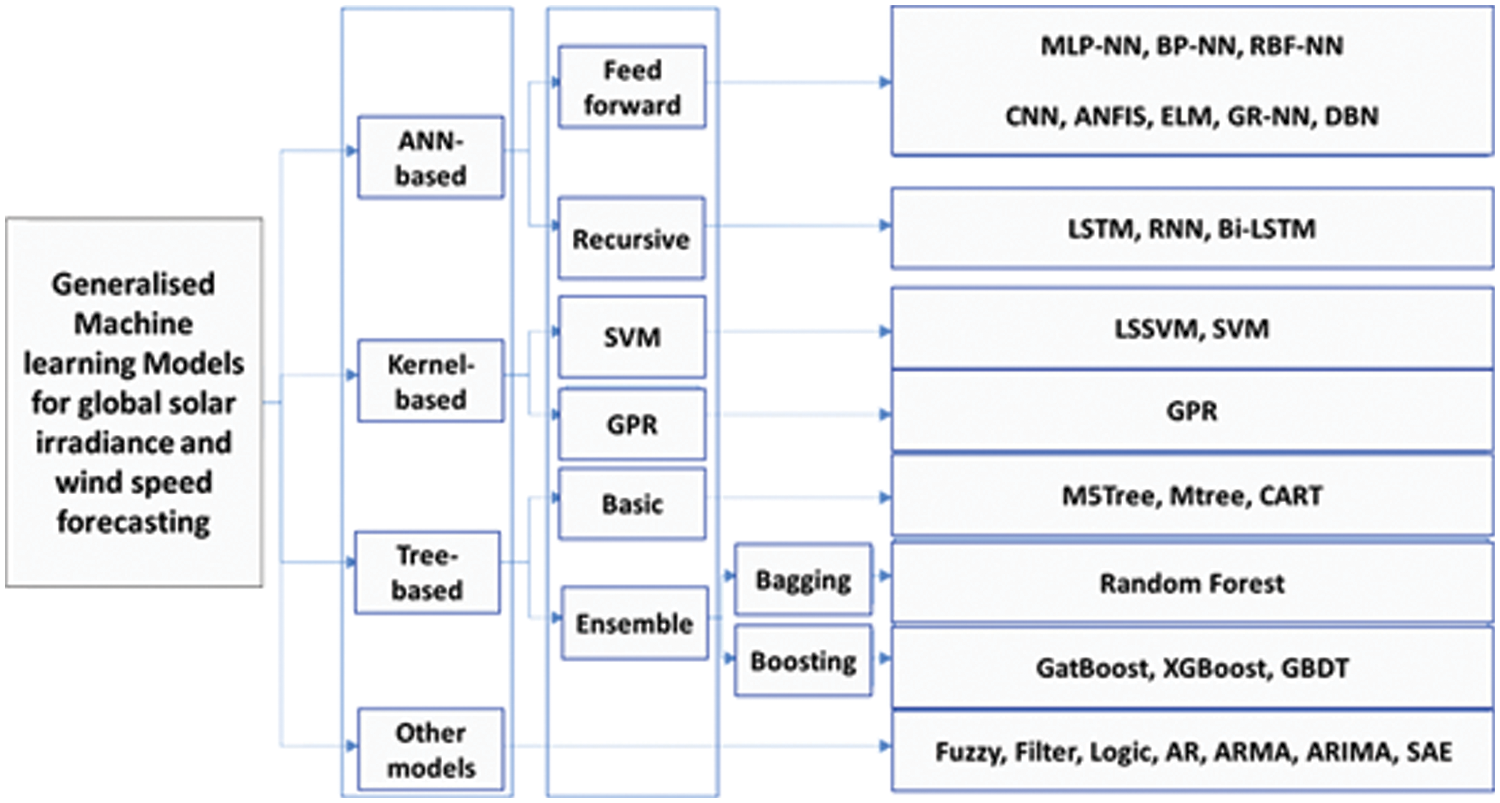
Figure 1: Machine learning models used for global solar irradiance and wind speed forecasting [30]
Kernel-based popular forecasting models include the “support vector machine” (SVM) [38], Least-squares SVM (LSSVM) [39], and Gaussian process regression (GPR). Tree-based solar irradiance and wind speed forecasting models can be categorized into “Gradient boosting decision tree” (GBDT), random forest, Model five tree (M5Tree), and “Classification and regression tree” (CART) [40]. The last category of other models includes autoregressive (AR), “Autoregressive moving average model” (ARMA), “Autoregressive integrated moving average model” (ARIMA) [41,42], SAEs, and fuzzy logic-based forecasting models [43].
As follows from the above literature, the described DL-based forecasting algorithms needed expertise to choose the correct number of data points, making the model less trustworthy and less effective in extracting nonlinear features. Some models also suffered from the problems of gradient disappearance, over-fitting, and excessive network training, while their lack of generalization capacity prevented them from learning complicated patterns. Moreover, the hyperparameters are not sufficiently finetuned to account for the lack of data. Therefore, the present study aimed to address these drawbacks by evaluating deep stacked S2AEs’ effectiveness in solar irradiation and wind speed time series prediction. It was necessary to test the effectiveness of Bi-LSTM-based deep-stacked S2SAE for wind speed and solar irradiance forecasting. Therefore, a novel Bi-LSTM-based deep stacked S2SAE for short-term solar irradiation and wind speed prediction was developed and evaluated in MATLAB. The forecasting performance of the proposed Bi-LSTM-based deep stacked S2SAE model was compared to three other deep and shallow stacked S2SAEs, i.e., the LSTM-based deep stacked S2SAE model, GRU-based deep stacked S2SAE model, and Bi-LSTM-based shallow stacked S2SAE model. Bayesian optimization was used to optimize the hyperparameters of all the forecasting models. The simulated results confirmed the superior performance of the proposed Bi-LSTM-based deep-stacked S2SAE forecasting model relative to other models.
The following section will explain the basic concepts of deep SAE and Bi-LSTM networks before detailing the proposed novel Bi-LSTM-based deep stacked S2SAE forecasting model for solar irradiance and wind speed forecasting.
Autoencoders are among the most significant neural network-based deep learning designs falling under unsupervised machine learning. They operate within three distinct layers: input, hidden, and output. Encoding is handled by the hidden layer, whereas decoding is performed by the output layer. The network is taught to produce a replica of the input. This is made possible by the hidden layer that learns the depictions of the inputs. Because autoencoders are taught to reproduce their input
When autoencoding, the autoencoder can be either under or over-complete. The hidden layer dimensions in an under-complete autoencoder are less than those in the input layer, whereas, in an over-complete autoencoder, they are more. The essential features of the inputs can be captured by an under-complete autoencoder. To train these networks, the backpropagation technique is used. Autoencoders can be used to represent either a linear or a nonlinear transformation. Under-complete autoencoders can be stacked and are used mainly in dimensionality reduction and data denoising [45]. When many autoencoders are stacked in a manner that uses each layer’s output as input to the next, a deep stacked under-complete autoencoder is obtained. The layers are trained unsupervised and independently of one another, and the results from one layer are used to train the next, as shown in Fig. 2. After all of the layers have been trained, the whole network undergoes supervised fine-tuning using backpropagation to optimize its performance by reducing the prediction error.
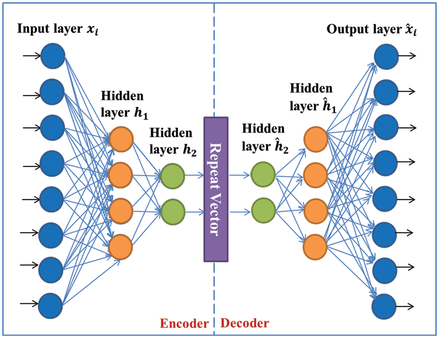
Figure 2: Basic-level architecture of proposed deep SAE
3.2 Deep Bi-directional Long Short-Term Memory Networks
To address the issue of vanishing gradients in RNNs, LSTM networks have been developed [46]. They achieve this by creating a model that can retain data for extended periods. Memory cells in an LSTM network typically include self-loops, as seen in Fig. 3. An input gate, forget gate, and output gate are depicted in the image as the three gates responsible for information flow in an LSTM cell. Memory cell states may be read via the output gate, written into via the input gate, and erased via the forget gate. The self-loops of an LSTM network allow for storing any sequential information that can be encoded on the state of the memory cell.
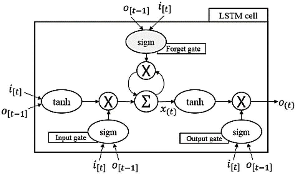
Figure 3: LSTM network single-cell structure [8]
The following equations describe how a single LSTM network cell functions [14]:
where
LSTM cells can be stacked on top of each other to create a deep or multi-layered network. Therefore, each LSTM layer consists of several hidden cells. The LSTM layers used in this study are bidirectional, meaning that the input sequence may be run either forwards or backward [47]. The number of memory cells is doubled in every layer of a Bi-LSTM network. Learning from past and future values gives it an edge over unidirectional LSTM. Fig. 4 depicts the Bi-LSTM layer architecture used in the present study. The difference between an LSTM and a Bi-LSTM layer is that the latter learns and remembers information from input in both the forward and reverse orientations. The forward direction is used to remember past input values, while the backward direction remembers future values. At every time step t, both historical and future data are accessible thanks to the combination of two hidden states storing the information separately (
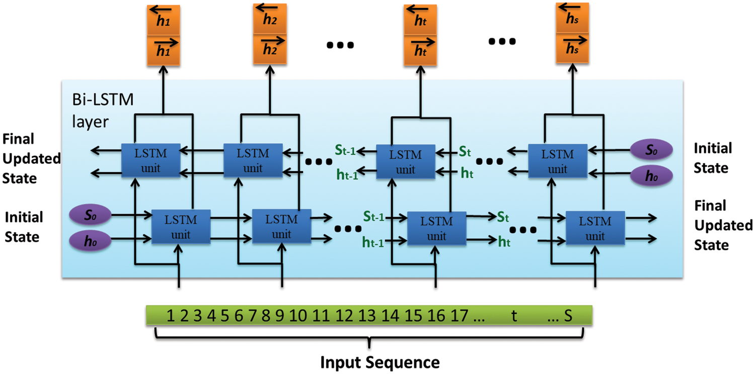
Figure 4: Bi-LSTM layer architecture used for developing a deep stacked autoencoder [14]
3.3 Proposed Bi-LSTM-Based Deep Stacked Autoencoder Sequence-to-Sequence Architecture
This study aimed to evaluate the effectiveness of a novel Bi-LSTM-based deep-stacked S2SAE designed for short-term predictions of both solar irradiation and wind speed. To create a deep-stacked S2SAE prediction model, six Bi-LSTM network layers were stacked on top of one another. The proposed deep model was inspired by [48], where the authors presented the first iteration of an RNN encoder-decoder. There are two main components to the proposed S2SAE methodology: an encoder and a decoder, as already shown in Fig. 2. Fig. 5 depicts the detailed architecture of the proposed Bi-LSTM-based deep stacked S2SAE. The encoder comprises three Bi-LSTM layers that take in the input sequence data, reduce its dimensions, and flatten it into a single vector, known as the repeat vector. This vector contains information about the complete input sequence and is repeated for t timesteps to reconstruct the original encoded sequence. The t timesteps represent the required number of future predictions [49].
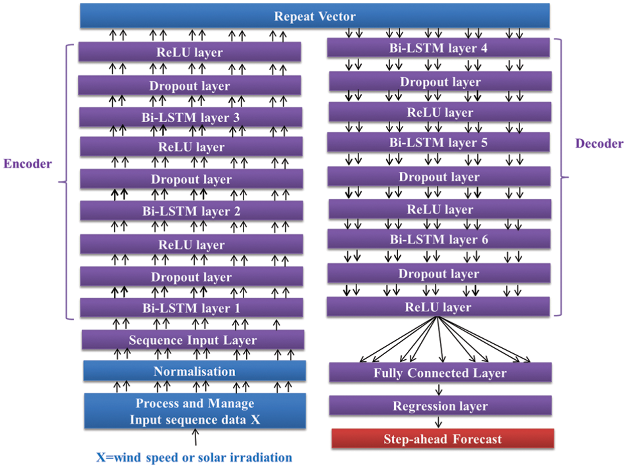
Figure 5: Proposed Bi-LSTM based deep stacked S2SAE
It is worth mentioning that the hidden states of every B-LSTM layer are fed as an input to a dropout layer, which is included to prevent the network from overfitting the data and consequently underperforming with novel values. The dropout layer is designed to operate at the probability of 0.05, which prevents overfitting by arbitrarily assigning 5% of inputs to zero. Similarly, the decoder is composed of three Bi-LSTM layers that receive this vector as an input and utilize it to generate a target sequence. The encoder uses Bi-LSTM cells to turn the input into a hidden state. Therefore, the hidden state of the most recent Bi-LSTM cell is the output vector generated by the encoder. Subsequently, the repeat vector’s reconstructed original sequence input is fed into the first Bi-LSTM-based hidden layer of the decoder. The layer uses this vector as its first hidden state, and the last time step’s output value is fed into the subsequent Bi-LSTM cell for the step-ahead forecast.
By gathering information from several Bi-LSTM layers, the model’s forecasting performance may enhance, and it can understand more complex representations of time-series data in the model’s hidden layers [50]. The outputs from the final dropout layer are sent to the fully connected layer, which converts the outputs into a single number representing the hour-ahead wind speed or solar irradiation for that time step. Finally, a regression output layer is linked so that the performance of the loss function can be tracked as the proposed Bi-LSTM-based deep stacked S2SAE network is being trained.
When developing an ML model, it is crucial to select optimum values of hyperparameters, i.e., parameters whose values are set before the model’s training begins. In RNN, hyperparameters generally include the maximum number of iterations, mini-batch size, number of hidden layers, initial learning rate, momentum, activation functions, and regularization factor. Model-specific considerations dictate specific hyperparameters to be used. There is no optimal set of hyperparameters common to all the models. In the presented study, these included the initial learning rate, the number of hidden neurons in every Bi-LSTM layer, and the L2 regularization (weight decay) factor. The initial learn-rate aids in finding generic patterns in the input sequence, and L2 regularization improves the model’s generalization and prevents overfitting, leading to more accurate forecasts. All the hyperparameters used were optimized using a Bayesian optimization method [51].
Bayesian optimization uses previous knowledge about the function and updates the knowledge gained via experimentation to minimize losses and increase the model’s accuracy. Other parameter-tuning methods, such as a grid and random search, were not used due to their inherent limitations. The shortcomings of a grid search become more apparent as the number of dimensions increases. In contrast, a random search is more akin to the greedy strategy because it stops at local optimum solutions rather than pursuing the global best [52]. These limitations can be solved with the help of Bayesian optimization, which efficiently reveals the black box function of the RNN’s global optima. It handles noisy input smoothly, exploits non-continuous regions, and scales effectively concerning these factors, allowing it to find global minima.
The activation function of a rectified linear unit “ReLU” was used with every Bi-LSTM layer while training the proposed deep stacked S2SAE forecasting model to deal with vanishing gradients. It also speeds up and improves the learning process [53]. In addition, Adam was selected as the optimization technique because it is fast, uses little memory, is resistant to gradient rescaling, and can deal with massive datasets [54]. The end of the training was determined based on two criteria: maximum epochs and early stopping. Early stopping is a regularization method which terminates training before a predetermined number of iterations have been completed by regulating validation loss. In MATLAB, the “ValidationPatience” parameter controls how many times a loss on the validation set can be greater than or equal to the previous lowest loss before the network training process is terminated. This parameter was set to 6, and the maximum number of epochs was 400. The training was automatically stopped when either of these stopping criteria was met.
Figs. 6 and 7 show the training progress of the proposed Bi-LSTM-based deep stacked S2SAE model for solar irradiation and wind speed forecasting, respectively, at optimum hyperparameter values. As is apparent, both training and validation losses and RMSEs were rather significant at the outset of the training but began to decrease as the epochs progressed. Generally, a forecasting model is said to be working effectively when the training and validation loss graphs meet at an intersection. Four hundred epochs were used in the model training, and from epoch 140 onwards in the case of solar irradiation and epoch 100 in the case of wind speed, and the training loss and validation loss curves were met. As such, the graph corroborates the performance of the proposed Bi-LSTM-based deep-stacked S2SAE model. However, for further performance validation and to support conclusions about the deep stacked S2SAE forecasting model’s efficacy in comparison to three other benchmark stacked S2SAEs, “mean absolute percentage error” (MAPE), RMSE, and R-squared (R2) performance metrics were calculated, as given in Eq. (3) [14]. Lower MAPE and RMSE would represent a better forecasting model, and R2 value closer to 1 would indicate a better fit between the forecasting model and the data given.
where
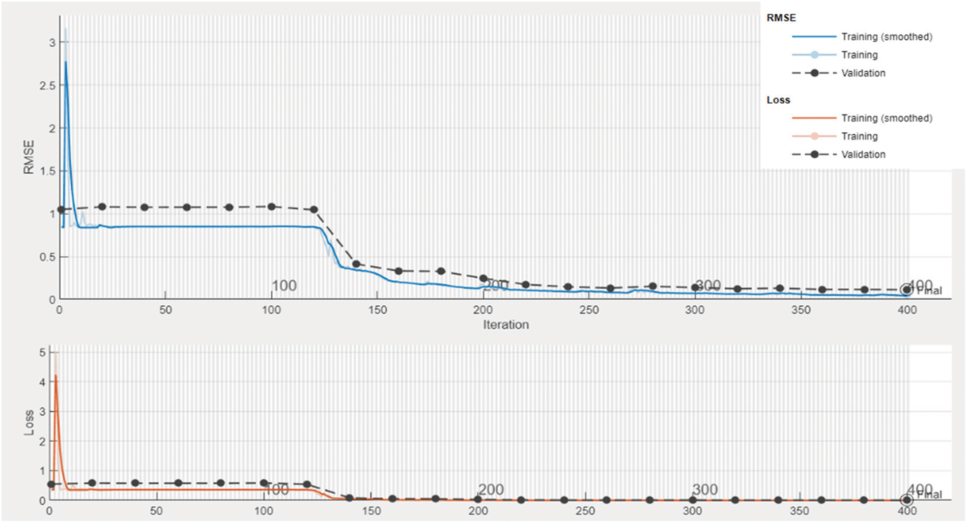
Figure 6: Training progress of proposed the Bi-LSTM-based deep stacked S2SAE model for solar irradiation forecasting
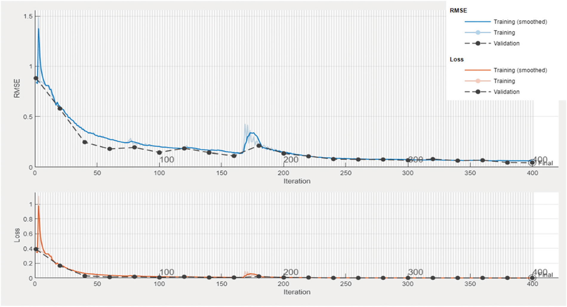
Figure 7: Training progress of the proposed Bi-LSTM-based deep stacked S2SAE model for wind speed forecasting
The forecasting performance of the proposed novel Bi-LSTM-based deep stacked S2SAE model for solar irradiation and wind speed forecasting was compared to three other deep and shallow stacked S2SAEs, i.e., the LSTM-based deep stacked S2SAE model, GRU-based deep stacked S2SAE model, and Bi-LSTM based shallow stacked S2SAE model. Shallow stacked S2SAE has one hidden layer after the input layer on the encoder side and one hidden layer before the output layer on the decoder side, whereas a deep stacked S2SAE has two hidden layers on both sides. All the above stacked S2SAE forecasting models were developed and optimized using Bayesian optimization in MATLAB.
All the models were evaluated relative to annual (January 2021 to January 2022) global horizontal irradiance (GHI) and wind speed hourly data obtained from the “NREL Solar Radiation Research Laboratory (BMS)” publicly available dataset [55]. To save computational time, 2,000 data points were used for training, validating, and testing the S2SAE forecasting models. In the case of solar irradiation stacked S2SAE forecasting models, the training data included hourly GHI readings (W/m2) from January 1, 2021, to March 11, 2021, and validation data included hourly GHI readings (W/m2) from March 12–18, 2021, and the testing data included hourly GHI readings (W/m2) from March 19–25, 2021. In the case of wind speed stacked S2SAE forecasting models, the training data included hourly wind speed readings (m/s) from January 1, 2021, to March 10, 2021, and validation data included hourly wind speed (m/s) from March 11–18, 2021, and the testing data included hourly wind speed (m/s) data from March 19–25, 2021. The GHI values from January 1–6, 2021, are shown in Fig. 8a), and the wind speeds from January 1–5, 2021, are shown in Fig. 8b). Moreover, as some values were missing from the wind data, they were pre-processed using the moving median method to complement the missing values.
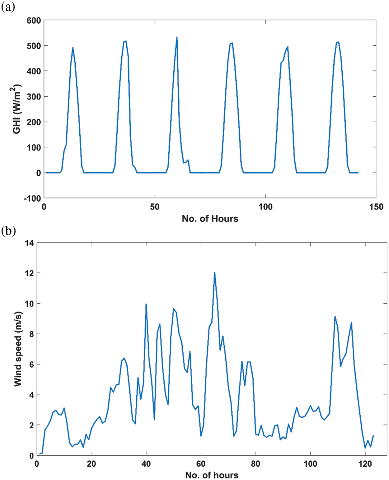
Figure 8: (a) GHI training dataset values (January 1–6, 2021) (b) Wind speed training dataset values (January 1–5, 2021)
The hyperparameters for each deep-stacked S2SAE forecasting model were optimized using at least 30 objective function evaluations using Bayesian optimization. The objective function was to minimize the MAPE. As deep learning models are sensitive to data scaling, the training and validation data were normalized to have unit variance and zero mean. MAPE measures the extent of the network’s underprediction or overprediction, and how successfully the network adopts new, unknown data is measured by the validation RMSE value. Therefore, the iteration with the lowest MAPE and validation RMSE values was selected as the optimal outcome of the experiment. Optimized hyperparameter values used for all the wind speed and solar irradiation forecasting Bi-LSTM-based deep stacked S2SAE models are shown in Table 1. Figs. 9 and 10 compare actual GHI and forecasted hour-ahead GHI values using the proposed Bi-LSTM-based deep-stacked S2SAE.
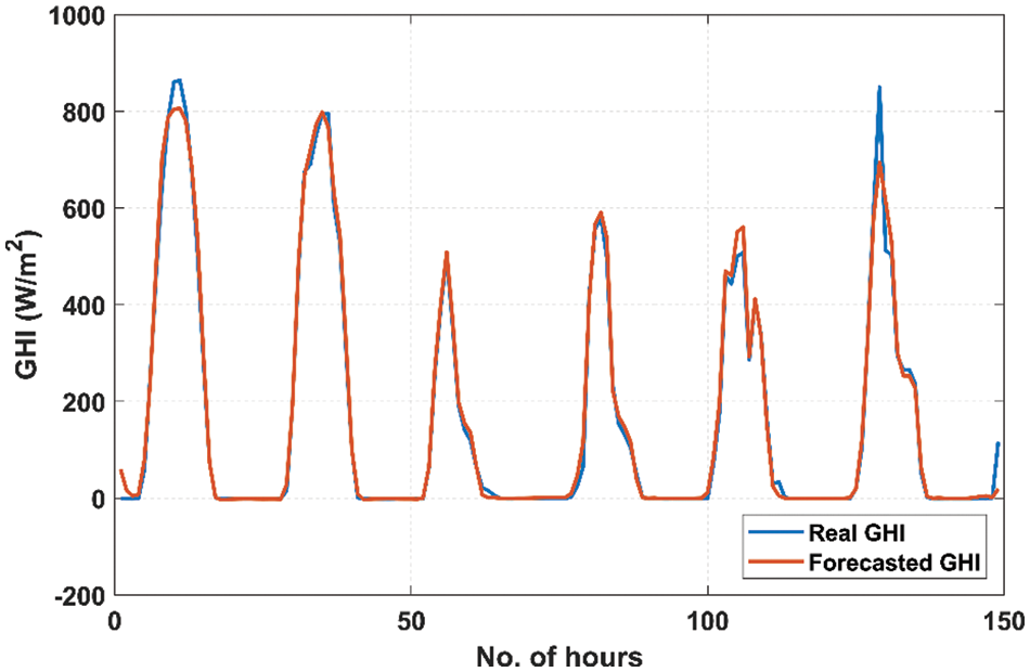
Figure 9: Comparison of actual GHI data with forecasted data using the proposed deep-stacked S2SAE
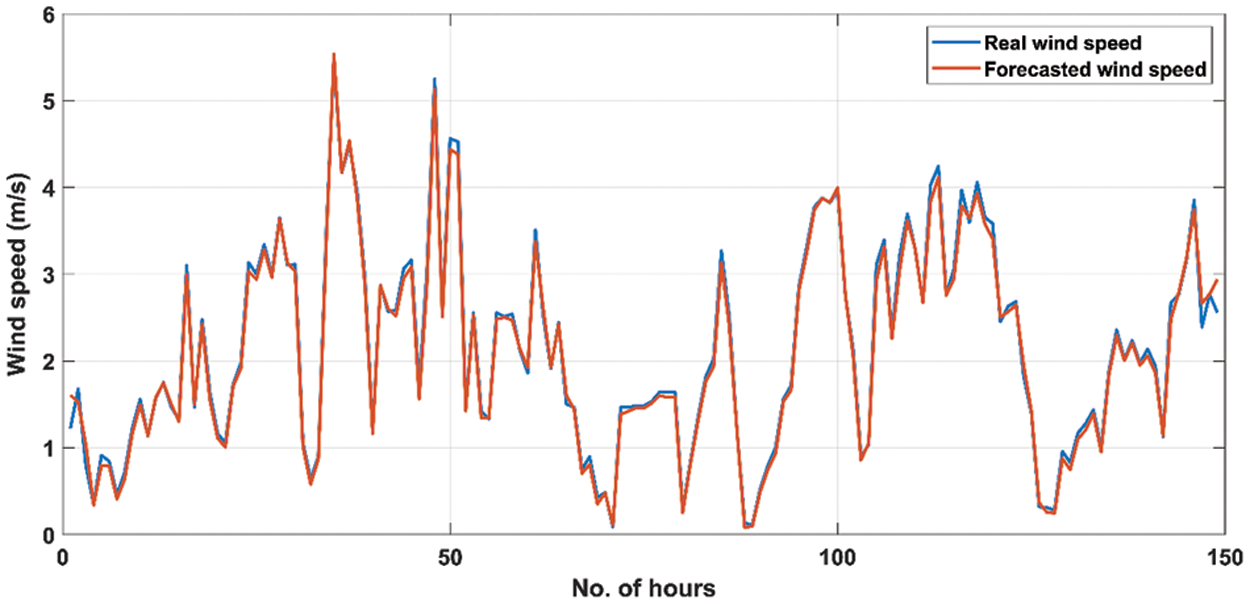
Figure 10: Comparison of actual wind speed data with forecasted data using the proposed deep-stacked S2SAE
Table 2 compares the forecasting performance of the proposed model to three other benchmark models. All the models were developed, trained, and implemented in MATLAB 2022a. It can be seen in Table 2 that in comparison to the other benchmark models, the proposed model achieved the lowest MAPE of 0.2763% when forecasting GHI and the lowest MAPE of 1.58% when forecasting wind speed. Similarly, in comparison to the other benchmark models, it was able to achieve the lowest RMSE value of 0.0358 when forecasting wind speed.
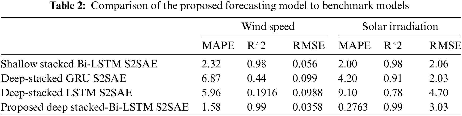
Moreover, when forecasting GHI, its RMSE value was 3.03, which was better than the LSTM-based deep stacked S2SAE and comparable to the GRU-based deep stacked S2SAE and Bi-LSTM-based shallow stacked S2SAE. Likewise, R-squared values reached 0.99 in both cases and were greater than the R-squared values for all the other models, confirming that the developed forecasting model is highly reliable. The lower values of MAPE indicate that the proposed Bi-LSTM deep stacked S2SAE-based forecasting model is 99.7% and 98.42% accurate for solar irradiation and wind speed forecasting, respectively. This would imply that the overall forecasts were only about 0.2763% and 1.58% off from the actual values. Similarly, lower RMSE values indicate that the observed data are very close to the predicted data.
Since the proposed Bi-LSTM-based deep stacked S2SAE can successfully learn crucial unobserved characteristics from time series and subsequently provide accurate predictions, we can confidently say that it is an effective method. The proposed Bi-LSTM-based deep encoder reducesthe input dimension and produces a single vector representation of input time sequence data. Next, the Bi-LSTM-based deep decoder uses this single vector to learn and generate the target sequence. The proposed deep-stacked S2SAE model was able to effectively reconstruct the input sequence and use the reconstruction error to forecast GHI and wind speed, demonstrating its high efficacy. Although LSTM and GRU are not affected by the vanishing gradient problem, they both overfitted and failed to capture the non-linearities in the time sequence data. At each time step, every single Bi-LSTM layer combines the results of the forward and backward layers to generate output. Moreover, unlike other prediction methods, every Bi-LSTM forecast is based on the entire data sequence. Another advantage of the proposed model is that the deep-stacked S2SAE is made without flip the source/target sequence since the Bi-LSTM layer can learn in both forward and reverse directions.
5 Conclusion and Future Research
A novel Bi-LSTM-based deep stacked S2SAE for short-term solar irradiation and wind speed predictions was developed and evaluated in MATLAB 2022a. The forecasting performance of the proposed Bi-LSTM-based deep stacked S2SAE model was compared to three other deep and shallow stacked S2SAEs, i.e., the LSTM-based deep stacked S2SAE model, GRU-based deep stacked S2SAE model, and Bi-LSTM based shallow stacked S2SAE model. Bayesian optimization was used to optimize the hyperparameters of all the forecasting models. The simulated results demonstrated the superiority of the proposed Bi-LSTM-based deep stacked S2SAE forecasting model over the other models. Compared to the other benchmark models, the proposed model achieved the lowest MAPE of 0.2763% when forecasting GHI and of 1.58% when forecasting wind speed. It was also able to achieve the lowest RMSE value of 0.0358 when forecasting wind speed. Moreover, the R-squared value reached 0.99 in both cases and was higher than in all the other models, confirming that the developed forecasting model is highly reliable. The presented study also explored the optimization of the initial learning rate, number of hidden neurons, and regularization factor at constant pre-defined values of other hyperparameters such as momentum and mini-batch size. On this basis, future research can consider optimizing such hyperparameters using nature-inspired algorithms such as artificial bee colony [56] or devising new transfer learning or reinforcement learning-based optimization algorithms.
Funding Statement: This research was funded by Warsaw University of Technology, Faculty of Mechanical and Industrial Engineering from funds for the implementation of KITT4SME (platform-enabled KITs of artificial intelligence for an easy uptake by SMEs) project. The project was funded under the European Commission H2020 Program, under GA 952119 (https://kitt4sme.eu/). The APC was funded by Warsaw University of Technology.
Conflicts of Interest: The authors declare that they have no conflicts of interest to report regarding the present study.
References
1. M. F. Zia, E. Elbouchikhi and M. Benbouzid, “Microgrids energy management systems: A critical review on methods, solutions, and prospects,” Applied Energy, vol. 222, no. 6, pp. 1033–1055, 2018. [Google Scholar]
2. A. Kuriqi, A. N. Pinheiro, A. Sordo-Ward and L. Garrote, “Water-energy-ecosystem nexus: Balancing competing interests at a run-of-river hydropower plant coupling a hydrologic-ecohydraulic approach,” Energy Conversion and Management, vol. 223, pp. 113267, 2020. https://doi.org/10.1016/j.enconman.2020.113267 [Google Scholar] [CrossRef]
3. A. Kuriqi, A. N. Pinheiro, A. Sordo-Ward and L. Garrote, “Flow regime aspects in determining environmental flows and maximising energy production at run-of-river hydropower plants,” Applied Energy, vol. 256, pp. 113980, 2019. [Google Scholar]
4. N. Suwal, X. Huang, A. Kuriqi, Y. Chen, K. P. Pandey et al., “Optimisation of cascade reservoir operation considering environmental flows for different environmental management classes,” Renewable Energy, vol. 158, no. 4, pp. 453–464, 2020. https://doi.org/10.1016/j.renene.2020.05.161 [Google Scholar] [CrossRef]
5. Q. Qdr, “Benefits of demand response in electricity markets and recommendations for achieving them,” US Dept. Energy, Washington, DC, USA, Tech. Rep, 2006. [Google Scholar]
6. A. D. Falehi, “An innovative optimal RPO-FOSMC based on multi-objective grasshopper optimization algorithm for DFIG-based wind turbine to augment MPPT and FRT capabilities,” Chaos Solitons & Fractals, vol. 130, pp. 109407, 2020. [Google Scholar]
7. A. DarvishFalehi, “An optimal second-order sliding mode based inter-area oscillation suppressor using chaotic whale optimization algorithm for doubly fed induction generator,” International Journal of Numerical Modelling: Electronic Networks, Devices and Fields, vol. 35, no. 2, pp. e2963, 2022. [Google Scholar]
8. L. Malka, A. Daci, A. Kuriqi, P. Bartocci and E. Rrapaj, “Energy storage benefits assessment using multiple-choice criteria: The case of Drini River Cascade, Albania,” Energies, vol. 15, no. 11, pp. 4032, 2022. [Google Scholar]
9. S. Kiliccote, D. Olsen, M. D. Sohn and M. A. Piette, “Characterization of demand response in the commercial, industrial, and residential sectors in the United States,” Advances in Energy Systems: The Large-scale Renewable Energy Integration Challenge, pp. 425–443, 2019. [Google Scholar]
10. M. Khalil, A. S. McGough, Z. Pourmirza, M. Pazhoohesh and S. Walker, “Machine learning, deep learning and statistical analysis for forecasting building energy consumption—A systematic review,” Engineering Applications of Artificial Intelligence, vol. 115, no. 11, pp. 105287, 2022. [Google Scholar]
11. K. M. Hamdia, X. Zhuang and T. Rabczuk, “An efficient optimization approach for designing machine learning models based on genetic algorithm,” Neural Computing and Applications, vol. 33, no. 6, pp. 1923–1933, 2021. [Google Scholar]
12. M. Alloghani, D. Al-Jumeily, J. Mustafina, A. Hussain and A. J. Aljaaf, “A systematic review on supervised and unsupervised machine learning algorithms for data science,” in Supervised and Unsupervised Learning for Data Science, Springer Cham: Switzerland, pp. 3–21, 2020. [Google Scholar]
13. F. Emmert-Streib, Z. Yang, H. Feng, S. Tripathi and M. Dehmer, “An introductory review of deep learning for prediction models with big data,” Frontiers in Artificial Intelligence, vol. 3, pp. 4, 2020. [Google Scholar] [PubMed]
14. N. Mughees, S. A. Mohsin, A. Mughees and A. Mughees, “Deep sequence to sequence Bi-LSTM neural networks for day-ahead peak load forecasting,” Expert Systems with Applications, vol. 175, pp. 114844, 2021. https://doi.org/10.1016/j.eswa.2021.114844 [Google Scholar] [CrossRef]
15. A. Rai, A. Shrivastava and K. C. Jana, “A robust auto encoder-gated recurrent unit (AE-GRU) based deep learning approach for short term solar power forecasting,” Optik, vol. 252, no. 3, pp. 168515, 2022. [Google Scholar]
16. Y. Yang, J. Zhong, W. Li, T. A. Gulliver and S. Li, “Semisupervised multilabel deep learning based nonintrusive load monitoring in smart grids,” IEEE Transactions on Industrial Informatics, vol. 16, no. 11, pp. 6892–6902, 2019. [Google Scholar]
17. S. Alwadei, A. Farahat, M. Ahmed and H. D. Kambezidis, “Prediction of solar irradiance over the Arabian Peninsula: Satellite data, radiative transfer model, and machine learning integration approach,” Applied Sciences, vol. 12, no. 2, pp. 717, 2022. [Google Scholar]
18. A. Di Piazza, M. C. Di Piazza, G. La Tona and M. Luna, “An artificial neural network-based forecasting model of energy-related time series for electrical grid management,” Mathematics and Computers in Simulation, vol. 184, no. 3, pp. 294–305, 2021. [Google Scholar]
19. A. Altan, S. Karasu and E. Zio, “A new hybrid model for wind speed forecasting combining long short-term memory neural network, decomposition methods and grey wolf optimizer,” Applied Soft Computing, vol. 100, no. 4, pp. 106996, 2021. [Google Scholar]
20. S. Ghimire, R. C. Deo, N. Raj and J. Mi, “Deep solar radiation forecasting with convolutional neural network and long short-term memory network algorithms,” Applied Energy, vol. 253, pp. 113541, 2019. [Google Scholar]
21. Y. -L. Hu and L. Chen, “A nonlinear hybrid wind speed forecasting model using LSTM network, hysteretic ELM and differential evolution algorithm,” Energy Conversion and Management, vol. 173, no. 2, pp. 123–142, 2018. [Google Scholar]
22. Jaseena K.U. and B. C. Kovoor, “EEMD-based wind speed forecasting system using bidirectional LSTM networks,” in 2021 Int. Conf. on Computer Communication and Informatics, ICCCI 2021, Coimbatore, India, pp. 1–9, 2021. [Google Scholar]
23. M. Alizamir, S. Kim, O. Kisi and M. Zounemat-Kermani, “A comparative study of several machine learning based non-linear regression methods in estimating solar radiation: Case studies of the USA and Turkey regions,” Energy, vol. 197, no. 1, pp. 117239, 2020. [Google Scholar]
24. A. Abayomi-Alli, M. O. Odusami, O. Abayomi-Alli, S. Misra and G. F. Ibeh, “Long short-term memory model for time series prediction and forecast of solar radiation and other weather parameters,” in 2019 19th Int. Conf. on Computational Science and Its Applications (ICCSA), St. Petersburg, Russia, pp. 82–92, 2019. [Google Scholar]
25. X. Liu and Z. Lin, “Impact of COVID-19 pandemic on electricity demand in the UK based on multivariate time series forecasting with bidirectional long short term memory,” Energy, vol. 227, pp. 120455, 2021. [Google Scholar] [PubMed]
26. M. H. Alsharif, M. K. Younes and J. Kim, “Time series ARIMA model for prediction of daily and monthly average global solar radiation: The case study of Seoul, South Korea,” Symmetry, vol. 11, no. 2, pp. 240, 2019. [Google Scholar]
27. A. Djaafari, A. Ibrahim, N. Bailek, K. Bouchouicha, M. Hassan et al., “Hourly predictions of direct normal irradiation using an innovative hybrid LSTM model for concentrating solar power projects in hyper-arid regions,” Energy Reports, vol. 8, no. 1187, pp. 15548–15562, 2022. [Google Scholar]
28. E. Jumin, F. B. Basaruddin, Y. B. Yusoff, S. D. Latif and A. N. Ahmed, “Solar radiation prediction using boosted decision tree regression model: A case study in Malaysia,” Environmental Science and Pollution Research, vol. 28, no. 21, pp. 26571–26583, 2021. [Google Scholar] [PubMed]
29. P. Kumari and D. Toshniwal, “Deep learning models for solar irradiance forecasting: A comprehensive review,” Journal of Cleaner Production, vol. 318, no. 3, pp. 128566, 2021. [Google Scholar]
30. Y. Zhou, Y. Liu, D. Wang, X. Liu and Y. Wang, “A review on global solar radiation prediction with machine learning models in a comprehensive perspective,” Energy Conversion and Management, vol. 235, pp. 113960, 2021. [Google Scholar]
31. Y. Amellas, O. El Bakkali, A. Djebli and A. Echchelh, “Short-term wind speed prediction based on MLP and NARX networks models,” Indonesian Journal of Electrical Engineering and Computer Science, vol. 18, no. 1, pp. 150–157, 2020. [Google Scholar]
32. Y. Zhang, B. Chen, Y. Zhao and G. Pan, “Wind speed prediction of IPSO-BP neural network based on lorenz disturbance,” IEEE Access, vol. 6, pp. 53168–53179, 2018. [Google Scholar]
33. R. H. J. Rani and T. A. A. Victoire, “Training radial basis function networks for wind speed prediction using PSO enhanced differential search optimizer,” PloS One, vol. 13, no. 5, pp. e0196871, 2018. [Google Scholar]
34. K. V. Shihabudheen and G. N. Pillai, “Wind speed and solar irradiance prediction using advanced neuro-fuzzy inference system,” in 2018 Int. Joint Conf. on Neural Networks (IJCNN), Rio de Janeiro, Brazil, pp. 1–7, 2018. [Google Scholar]
35. M. S. Syed, C. V. Suresh and S. Sivanagaraju, “Short term solar insolation prediction: P-ELM approach,” International Journal of Parallel, Emergent and Distributed Systems, vol. 33, no. 6, pp. 663–674, 2018. [Google Scholar]
36. M. M. Lotfinejad, R. Hafezi, M. Khanali, S. S. Hosseini, M. Mehrpooya et al., “A comparative assessment of predicting daily solar radiation using bat neural network (BNNgeneralized regression neural network (GRNNand neuro-fuzzy (NF) system: A case study,” Energies, vol. 11, no. 5, pp. 1188, 2018. [Google Scholar]
37. M. Wang, H. Zang, L. Cheng, Z. Wei and G. Sun, “Application of DBN for estimating daily solar radiation on horizontal surfaces in Lhasa, China,” Energy Procedia, vol. 158, no. 1, pp. 49–54, 2019. [Google Scholar]
38. S. Gangwar, V. Bali and A. Kumar, “Comparative analysis of wind speed forecasting using LSTM and SVM,” EAI Endorsed Transactions on Scalable Information Systems, vol. 7, no. 25, pp. 1–9, 2020. [Google Scholar]
39. A. Zendehboudi, M. A. Baseer and R. Saidur, “Application of support vector machine models for forecasting solar and wind energy resources: A review,” Journal of Cleaner Production, vol. 199, pp. 272–285, 2018. [Google Scholar]
40. J. Moon, Z. Shin, S. Rho and E. Hwang, “A comparative analysis of tree-based models for day-ahead solar irradiance forecasting,” in 2021 Int. Conf. on Platform Technology and Service (PlatCon), Jeju, Korea, pp. 1–6, 2021. [Google Scholar]
41. H. Suyono, D. O. Prabawanti, M. Shidiq, R. N. Hasanah, U. Wibawa et al., “Forecasting of wind speed in Malang City of Indonesia using adaptive neuro-fuzzy inference system and autoregressive integrated moving average methods,” in 2020 Int. Conf. on Technology and Policy in Energy and Electric Power (ICT-PEP), Bandung, Indonesia, pp. 131–136, 2020. [Google Scholar]
42. K. Palomino, F. Reyes, J. Núñez, G. Valencia and R. H. Acosta, “Wind speed prediction based on univariate ARIMA and OLS on the Colombian Caribbean coast,” Journal of Engineering Science and Technology Review, vol. 13, no. 3, pp. 200–205, 2020. [Google Scholar]
43. D. Shah, K. Patel and M. Shah, “Prediction and estimation of solar radiation using artificial neural network (ANN) and fuzzy system: A comprehensive review,” International Journal of Energy and Water Resources, vol. 5, no. 2, pp. 219–233, 2021. [Google Scholar]
44. U. R. Alo, H. F. Nweke, Y. W. Teh and G. Murtaza, “Smartphone motion sensor-based complex human activity identification using deep stacked autoencoder algorithm for enhanced smart healthcare system,” Sensors, vol. 20, no. 21, pp. 6300, 2020. [Google Scholar] [PubMed]
45. P. Thomadakis, A. Angelopoulos, G. Gavalian and N. Chrisochoides, “De-noising drift chambers in CLAS12 using convolutional auto encoders,” Computer Physics Communications, vol. 271, no. 4, pp. 108201, 2022. [Google Scholar]
46. S. Bouktif, A. Fiaz, A. Ouni and M. Serhani, “Optimal deep learning lstm model for electric load forecasting using feature selection and genetic algorithm: Comparison with machine learning approaches,” Energies, vol. 11, no. 7, pp. 1636, 2018. [Google Scholar]
47. X. Tang, Y. Dai, T. Wang and Y. Chen, “Short-term power load forecasting based on multi-layer bidirectional recurrent neural network,” IET Generation, Transmission and Distribution, vol. 13, no. 17, pp. 3847–3854, 2019. [Google Scholar]
48. K. Cho, B. Van Merriënboer, C. Gulcehre, D. Bahdanau, B. Fethi et al., “Learning phrase representations using RNN encoder-decoder for statistical machine translation,” in EMNLP 2014—2014 Conf. on Empirical Methods in Natural Language Processing, Proc. of the Conf., Doha, Qatar, pp. 1724–1734, 2014. [Google Scholar]
49. G. Gong, X. An, N. K. Mahato, S. Sun, S. Chen et al., “Research on short-term load prediction based on Seq2seq model,” Energies, vol. 12, no. 16, pp. 3199, 2019. [Google Scholar]
50. S. Hwang, G. Jeon, J. Jeong and J. Lee, “A novel time series based Seq2Seq model for temperature prediction in firing furnace process,” Procedia Computer Science, vol. 155, no. 9, pp. 19–26, 2019. [Google Scholar]
51. A. H. Victoria and G. Maragatham, “Automatic tuning of hyperparameters using Bayesian optimization,” Evolving Systems, vol. 12, no. 1, pp. 217–223, 2021. [Google Scholar]
52. Y. Sun, B. Xue, M. Zhang and G. G. Yen, “An experimental study on hyper-parameter optimization for stacked auto-encoders,” in 2018 IEEE Congress on Evolutionary Computation (CEC), Rio de Janeiro, Brazil, pp. 1–8, 2018. [Google Scholar]
53. S. R. Dubey, S. K. Singh and B. B. Chaudhuri, “Activation functions in deep learning: A comprehensive survey and benchmark,” Neurocomputing, vol. 503, no. 11, pp. 92–108, 2022. [Google Scholar]
54. D. P. Kingma and J. Ba, “Adam: A method for stochastic optimization,” arXiv preprint arXiv: 1412. 6980, 2014. [Google Scholar]
55. T. Andreas and A. Stoffel, “NREL Solar radiation research laboratory (SRRLBaseline measurement system (BMS); Golden, Colorado (Data); NREL Report No. DA-5500-56488,” 2022. [Online]. Available: https://doi.org/10.5439/1052221 [Google Scholar] [CrossRef]
56. A. Mughees and S. A. Mohsin, “Design and control of magnetic levitation system by optimizing fractional order PID controller using ant colony optimization algorithm,” IEEE Access, vol. 8, pp. 116704–116723, 2020. [Google Scholar]
Cite This Article
 Copyright © 2023 The Author(s). Published by Tech Science Press.
This work is licensed under a Creative Commons Attribution 4.0 International License , which permits unrestricted use, distribution, and reproduction in any medium, provided the original work is properly cited.
 Downloads
 Citation Tools