Image Generation of Tomato Leaf Disease Identification Based on Small-ACGAN

1  Introduction

Plant diseases are a common natural phenomenon that compromises plants’ survival and reproduction. According to the Food and Agriculture Organization (FAO), up to 40% of food crops are destroyed by plant pests and diseases each year, costing the global economy more than $220 billion [1]. For example, as a widely and efficiently cultivated and valuable crop with rich nutritional and economic value, tomatoes might be infected with different diseases, thus negatively impacting the yield and quality of their fruits [2]. Accurate identification of tomato diseases is a critical step for early prevention and control of such damage.

With the progress in artificial intelligence, deep learning for data analytics and image processing has become a rapidly growing field. As an integral branch of deep learning, Convolutional neural networks have made even more significant breakthroughs in detecting and classifying plant leaf diseases [3]. For example, Mohanty et al. [4] used GoogLeNet [5] to identify 26 species with a total of 54,306 leaves and an accuracy of 99.35% on a held-out test set but poor accuracy on another dataset. Ghosal et al. [6] proposed a VGG-16 [7] based CNN architecture, which led to an accuracy of 92.46% on a dataset of rice leaf diseases with a total of 2,156 images in four classes. Jiang et al. [8] used the CNN model ResNet50 and achieved an accuracy of 98.0% on a total of 3,000 datasets for three tomato diseases. However, to improve their accuracy and generalization ability, such networks require a large amount of well-labeled data to train models. Unfortunately, many plant datasets have solid issues, such as uneven distribution or small quantity of leaves per plant type [9]. The main reason is that leaf images are not easy to collect in the case of plant leaf diseases. This results in insufficient datasets to accurately reflect the actual situation. In addition, identifying diseases also requires expertise since it is a highly challenging part of the process. All of those potential issues reflect that research into improving identification accuracy based on small datasets with existing labels is a topic worth exploring within the academic community.

Due to the difficulties in acquiring data samples, some researchers use rotation, blurring, contrast, scaling, illumination, and projection transformations [10] on images to expand datasets and avoid overfitting and low generalization due to insufficient data. However, these results are still simple changes to the original images, making no remarkable improvement to identification accuracy. In order to solve such problems, this paper proposes a novel small-ACGAN model through which data enhancement of plant disease leaves is performed to generate higher-quality images than ACGAN [11] to solve the minor sample recognition problems. The main contributions of this study are summarized as follows:

 1)   The proposal of a small ACGAN that can effectively expand the dataset based on several datasets. First, CA [12] is used in the generator to make the generated images better and the model relatively small. Secondly, the loss function of the discriminator is optimized, and a gradient penalty is added to it to make the training process more stable, improve the model’s generalization ability and alleviate the overfitting problem.

 2)   The dataset is doubled by Generative Adversarial Network (GAN) [13], and the generated images are mixed with the original images as the training set. The results proved that the doubled dataset obtained higher accuracy in the recognition performance of the classification model of CNN, and both exceeded the initial dataset.

 3)   By comparing the accuracy of Deep Convolution GAN (DCGAN) [14], Wasserstein GAN with gradient penalty (WGAN-GP) [15], conditional GAN (CGAN) [16], Faster and Stabilized GAN (FastGAN) [17], and small-ACGAN on three CNN models, it is proved that the method proposed in this paper is indeed more efficient.

 4)   Grape and apple datasets were used to validate the effectiveness and generalizability of small-ACGAN after augmentation.

This paper is structured as follows. Section 1 introduces plant diseases and the need for timely detection; Section 2 presents a literature review on data amplification; Section 3 describes the methods used in this paper; Section 4 describes the experiments and analyzes the results; and Section 5 gives the conclusions.

2  Related Work

2.1 Data Expansion

In the field of deep learning in agriculture, a considerable number of datasets is necessary to improve the performance of network models. However, what we do occasionally notice is that the data available are not sufficient. To address this problem, some researchers have tried to expand their datasets and have obtained better accuracy.

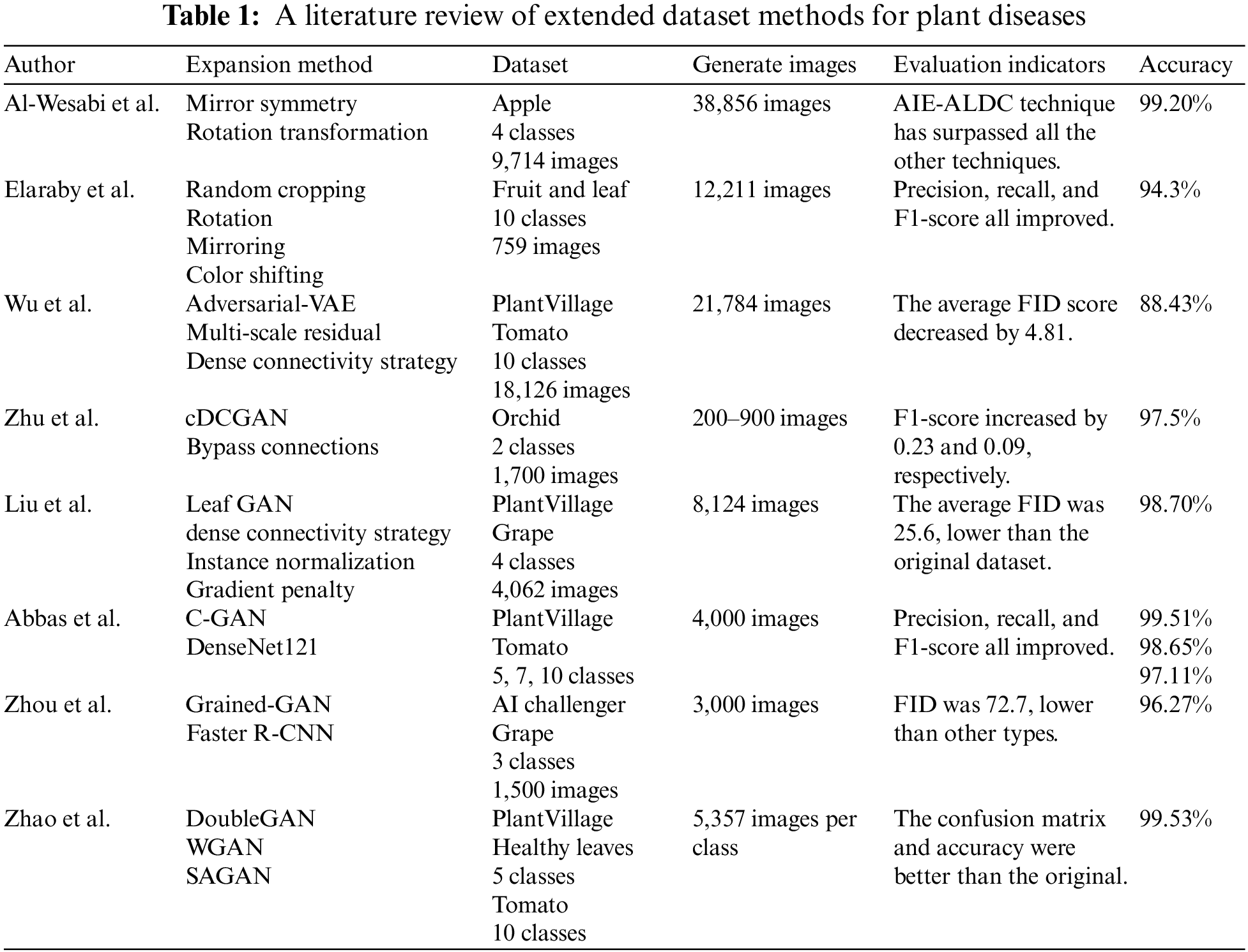
Al-Wesabi et al. [18] proposed an efficient Artificial Intelligence Enabled Apple Leaf Disease Classification (AIE-ALDC) technique, which expanded the dataset by four times using mirror symmetry and rotation transformation based on a random point of the image. They applied a Gaussian function to enhance the image quality, followed by feature extraction with the water wave optimization-capsule network (WWO-CapsNet) [19,20], and then classification with the bidirectional long short-term memory (BiLSTM) [21]. Finally, this method resulted in an accuracy of 99.2% for apple leaf disease identification.

Elaraby et al. [22] improved the optimizer using stochastic gradient descent dynamics (SGDM). Then, with random cropping, rotation, mirroring, and color conversion, 759 images were enhanced to 12,211 with a maximum accuracy of 94.3%. Taking a multi-scale residual learning module, Wu et al. [23] extracted leaf features and integrated a dense connectivity strategy into Adversarial Variational Auto-Encoder (Adversarial-VAE), aiming to generate better-performing tomato disease images.

2.2 Data Expansion Based on GAN

Data augmentation methods generally adopt GAN, which can well illustrate the great advantage of GAN networks in image generation. Overall, a GAN network means two models: one is a generator, and the other is a discriminator. The former creates a near-real image, while the latter determines the image’s authenticity, and they do confrontation training together. In addition, the former has to continuously optimize the generated images so that the latter cannot judge them. The latter, on the other hand, has to optimize itself to make its judgments more accurate. Along with the adversarial training, the two models would become more vital, finally reaching smoothness [13].

Zhu et al. [24] modified conditional deep convolutional GAN (cDCGAN) by adding bypass connections and then strengthened the orchid dataset based on the specified category labels resulting in high-quality fine-grained RGB orchid images. The method expanded the dataset to different multiples and eventually found that the best results were achieved when the number of images increased to 800. The F1 scores for the two datasets increased by 0.23 and 0.09, respectively, with an accuracy of up to 97.5%.

Liu et al. [25] designed a channel-decreasing generator model to derive images. This approach extended twice for a grape dataset with the average Fréchet Inception Distance (FID) [26] of 235.81, which was 25.6 lower than the original dataset. The highest accuracy of the generator reached 98.7%.

Abbas et al. [27] generated synthetic images of tomato leaves by using CGAN and trained a DenseNet121 [28] model based on migration learning. After generating 4,000 images in his way, he mixed them into a tomato training set and classified the leaf images into 5, 7, and 10 classes for each experiment. We also find that the accuracy, recall, and F1 scores are increased compared to the original dataset, with the final precision reaching 99.51%, 98.65%, and 97.11%, respectively. Zhou et al. [29] proposed a grained-GAN to improve Faster Region-based Convolutional Network (Faster R-CNN) [30]. The model generated 1,000 local speckle region sub-images for each category, all of which showed lower FIDs than the GANs of other categories. All five network models finally showed high identification accuracy, with the highest reaching 96.72%.

Zhao et al. [31] proposed DoubleGan by incorporating two GANs. First, WGAN inputted healthy leaves to obtain a pre-trained model; then, the sick leaves were through the pre-trained model for elimination. Later, it applied Self-Attention-GAN (SAGAN) [32] to generate images to expand the dataset. It scaled up to 5,357 leaves of each type and compared them with the original and flipped extended datasets. The experimental results showed a higher accuracy than the original dataset, except for one category, which delivered a slightly lower accuracy. Moreover, the confusion matrix was also influential, with an accuracy of 99.53%.

Table 1 summarizes the methods, the number of generated images, and the accuracy of the expanded plant datasets acquired in the literature above. It is evident from the dataset and generated image columns in Table 1 that all of these methods have a common issue with the need for a large dataset. However, this paper relies on a small dataset for experiments. Moreover, by reading the previously mentioned papers, we found that the expansion multiples of the datasets also differed. Al-Wesabi et al. [18] expanded the dataset four times, Zhu et al. [24] and also Liu et al. [25] expanded it twice, and Abbas et al. [27] expanded it 0.25 times. One of the main focuses of this paper is the frequency of the extension process.

3  Materials and Methods

3.1 Dataset

This paper focused on the tomato dataset publicly available in PlantVillage [33] as the object of study. The dataset contains 18,159 images in ten categories, covering nine types of diseased leaves and one type of healthy leaves. As shown in Table 2, its dataset distribution is still very uneven, with the number of TYL images 14 times more than that of TMV, which can impact the training of the network. Therefore, many studies tend to eliminate datasets with few images to improve accuracy.

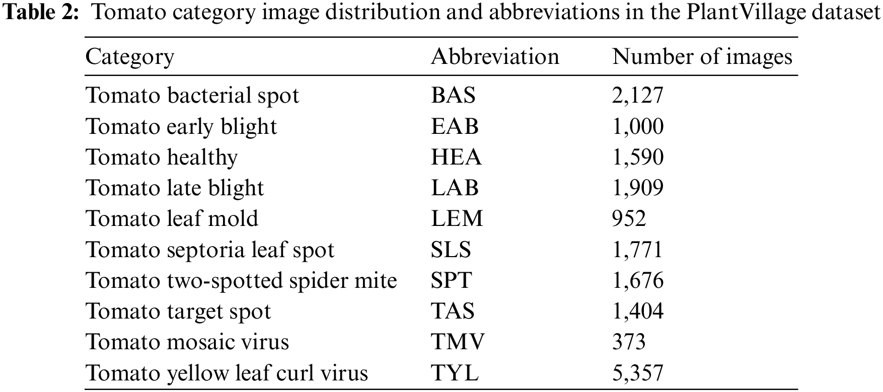
A category of plant leaves may contain only a few dozen or a few hundred images in many datasets. This paper is divided into a training set, a validation set, and a test set in the ratio of 1:1:1 for 300 images selected from each disease category in order to demonstrate that the proposed method can effectively enhance the recognition ability of the network even with a minimum number of data sets. For the convenience of reading and understanding, the names of the tomato leaf diseases are abbreviated, as shown in the second column of Table 2.

3.2 ACGAN

ACGAN is used to extend the dataset in this paper to prevent network overfitting. There are many GAN networks available for data augmentation. For instance, Abbas and Zhu [24,27] used C-GAN and DCGAN, respectively, for data augmentation. However, ACGAN used in this study combined the advantages of them. As to the time of input, compared to C-GAN, ACGAN can make training with labels and reconstruct labels, in addition to generating specific labeled data; moreover, labels can be submitted as feedback to the learning ability of the discriminative network at the time of judgment. Regarding feature extraction, ACGAN resembles DCGAN. It takes a deep convolutional network to perform better extraction of feature values of images, and yet it differs from DCGAN in that it adds image labels.

The architecture diagram of the optimized small-ACGAN in this paper is shown in Fig. 1. The small-ACGAN consists of two kinds of adversarial networks: the generator and discriminator models. The former is mainly to generate fake data as accurately as possible, while the latter is mainly to distinguish the real and fake datasets and determine the categories. If the model is well-trained, the generator will create near-realistic fake images that could scale the dataset nicely. In contrast to CGAN, the loss function of ACGAN is divided into two parts: true-false  LS and classification loss LC. Eqs. (1)–(4) are from ACGAN [11].

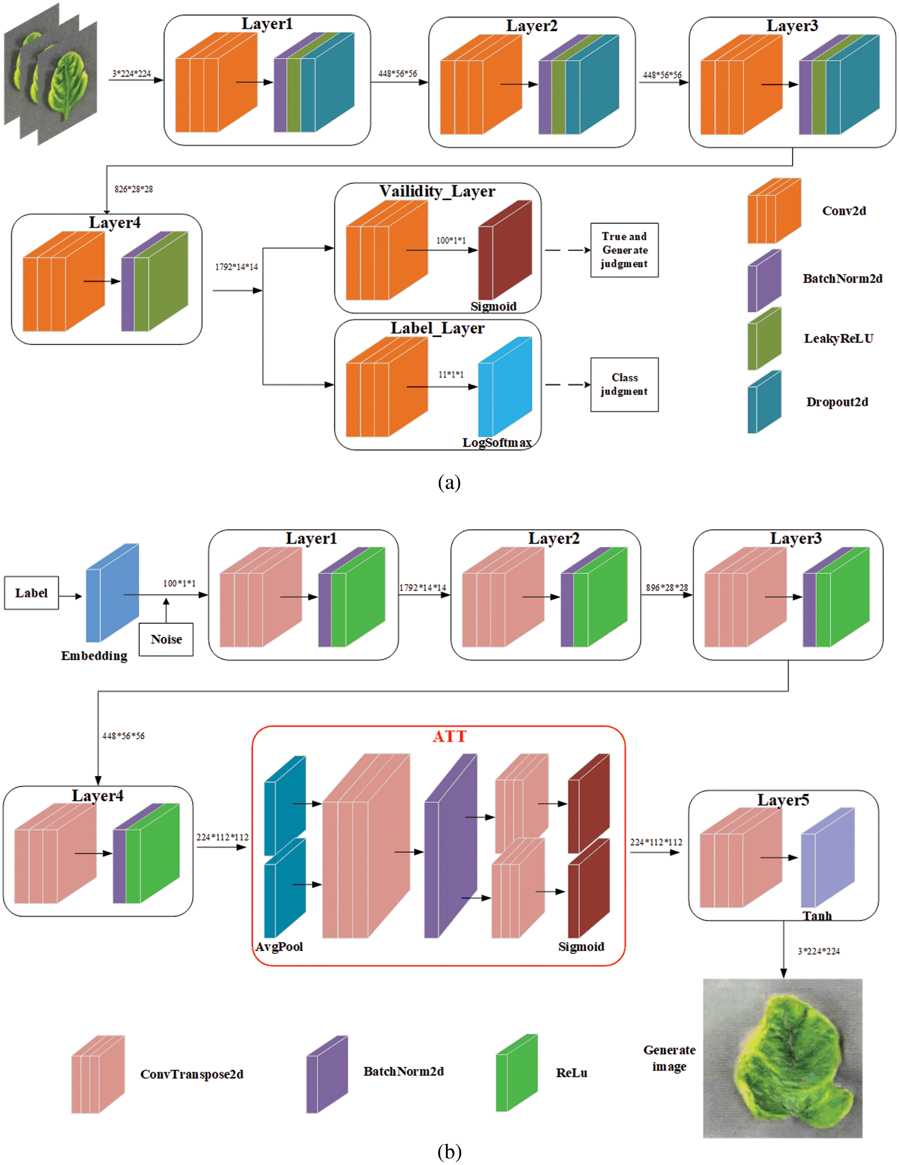
Figure 1: Architecture diagram of small-ACGAN. (a) Discriminator (b) generator

In the aspects of true and false losses:

LS=E[log⁡P(S=real|Xreal)]+E[log⁡P(S=fake|Xfake)](1)

In the aspects of classification loss:

LC=E[log⁡P(C=c|Xreal)]+E[log⁡P(C=c|Xfake)](2)

Eq. (3) is the overall loss of the generator. In order to increase the realism of the image, this method must maximize LC and minimize LS. Eq. (4) is the overall loss of the discriminator. In order to increase the classification accuracy of the discriminator, LD needs to be maximized. The two models become more robust than each other.

LG=LC−LS(3)

LD=LC+LS(4)

3.3 Coordinate Attention

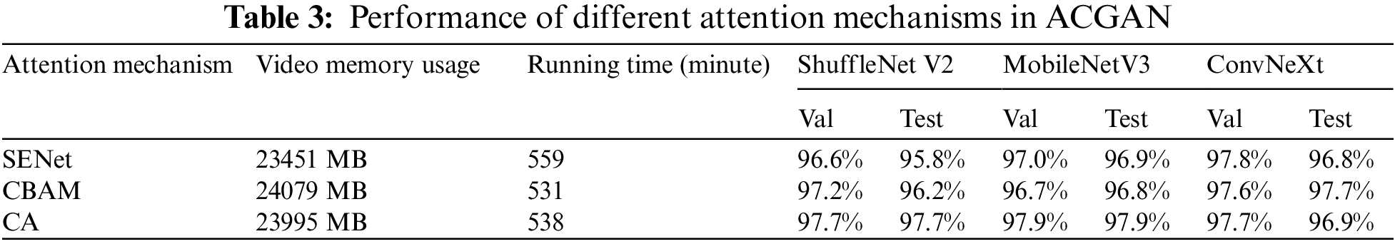
Aiming to investigate the effect of the attention mechanism on the performance of ACGAN, this section conducts comparative experiments on three attention mechanisms, namely Squeeze-and-Excitation Networks (SENet) [34], Convolutional Block Attention Module (CBAM) [35], and CA. It is worth mentioning that all three models are the same except for the attention mechanism. Table 3 shows the comparative results. SENet occupies the little memory and takes the longest time to run, CBAM occupies the most significant memory but takes the shortest time, and CA is in the middle regarding memory size and running time. In classification models, ShuffleNet V2 [36], MobileNetV3 [37], and ConvNeXt [38] all had high accuracy on CA. Therefore, it was suitable to use CA as the primary attention mechanism.

In Fig. 1b, the red box circled is the CA module in small-ACGAN. It decomposes channel attention into two parallel 1D feature encoding processes to efficiently integrate spatial coordinate information into the generated attention maps. One method captures long-range dependencies along one spatial orientation, and the other retains accurate location information. The generated feature maps are then encoded separately to form a pair of direction-aware and location-sensitive feature maps. These can be complementarily applied to the input feature maps to enhance the representation of the targets of interest. Eqs. (5)–(10) are from CA [12].

Specifically, the input feature map X is encoded along the horizontal and vertical coordinate directions using average pooling to obtain feature maps in both the width and height directions, as shown in Eqs. (5) and (6):

zch(h)=1W∑0≤i<Wxc(h,i)(5)

zcw(w)=1H∑0≤j<Hxc(j,w)(6)

Then, the global perceptual field feature maps obtained from Eqs. (5) and (6) are stitched together and fed into the convolution module with a convolution kernel of 1 * 1 to reduce its dimension to the original C/r. Then, the batch-normalized feature map F1 is input into the Sigmoid activation function to obtain the feature map f, as shown in Eq. (7).

f=δ(F1([zh,zw]))(7)

The feature map f is convolved with a 1 × 1 kernel by the original height and width to obtain the feature maps fh and fw with the same number of channels as the original feature map, respectively. Then, the attention weights gh and gw for the height and width directions of the feature map are obtained by the Sigmoid activation function, shown in Eqs. (8) and (9).

gh=σ(Fh(fh))(8)

gw=σ(Fw( fw))(9)

After the above calculation, the attention weights of the input feature map in the height direction and the attention weights in the width direction are obtained. Finally, multiplying and weighting the original feature map will obtain the final feature map with attention weights in the width and height directions, as shown in Eq. (10).

yc(i,j)=xc(i,j)×gch(i)×gcw(j)(10)

3.4 Optimizing the Loss Function

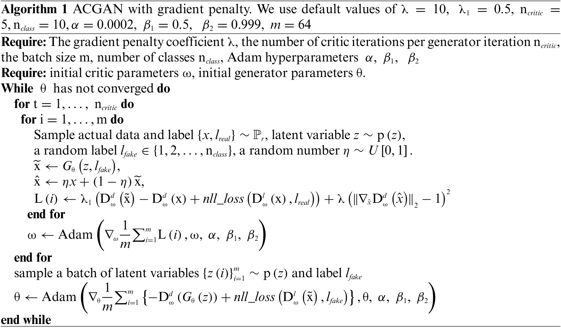
In order to prevent the problem of model collapse and gradient explosion during training, this paper adds a gradient penalty to the loss function of the discriminator of small-ACGAN. This method can link the problem of gradient explosion and make weight correction adaptively, making the training process more stable. In addition, it allows the model to converge faster, improves its generalization ability [15], alleviates the overfitting problem, and produces higher-quality graphs. Algorithm 1 describes the ACGAN with a modified loss function procedure.

Eq. (11) shows the loss calculation for the gradient penalty module. ∇xD(x) denotes the gradient of the discriminator output value in the x-direction. Ex−x^ denotes the mathematical expectation when the input to the discriminator is a randomly interpolated sample x^.

LGP=Ex−x^[(∥∇xD(x)∥2−1)2](11)

The loss of small-ACGAN in this study is shown in Eq. (12). With the adoption of the gradient penalty mechanism, LD can be updated as follows:

LD=(LC+LS)∗0.5+lam_gp∗ LGP(12)

where lam_gp is the hyperparameter and is set to 10 in all experiments.

4  Results

4.1 Experimental Environment

In the experimental section, this paper has used Python 3.8, and the experiment was performed on ubuntu18.04, accelerated by GPU RTX 3090 24G. Table 4 shows the specific parameters used during the experiment, divided into two main experimental sections. One part is assigned to train small-ACGAN. The other part specializes in image classification and utilizes the same parameters in the training and testing of the AlexNet, VGG-16, MobileNetV3, ShuffleNet V2, and ConvNeXt models used in this paper. The same data enhancements, such as panning, rotating, flipping, and scaling, are applied to all images during training and testing.

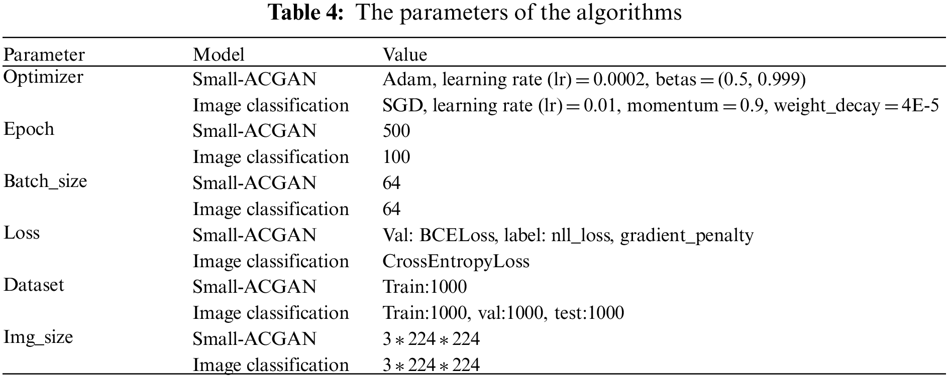
The learning rate is one of the most critical hyperparameters in deep learning. The SGD optimizer works for image classification, so the weight_decay and learning rate are available to calculate the loss value for each batch of samples. Then, the learning rate is updated by the average gradient of the batch. Furthermore, this paper set the momentum [39] to 0.9 so that the update retains the direction of the previous update to a certain extent, which increases the stability and makes the model learn faster with the ability to get rid of the local optimum. Fig. 2 shows the change in the learning rate as the number of training sessions of MobileNetV3 increases.

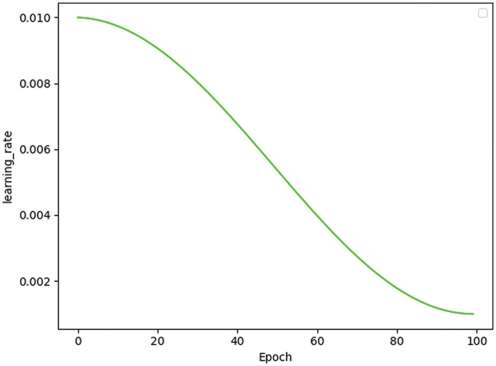
Figure 2: Learning rate change in MobileNetV3

4.2 Evaluation

This study employed the metrics commonly adopted in classification tasks to evaluate the method’s performance. Some methods used were: Accuracy, Precision, Recall, F1 Score, Precision-Recall Curve (P-R Curve), Receiver Operating Characteristic Curve (ROC), Area Under Curve (AUC), and Confuse Matrix. Performance measures can be calculated using the equations from Eqs. (13)–(16).

Accuracy=TP+TNTP+TN+FP+FN(13)

Precision=TPTP+FP(14)

Recall=TPTP+FN(15)

F1−score=2Precision∗RecallPrecision+Recall(16)

where TP = True Positive, TN = True Negative, FP = False Positive, and FN = False Negative.

The ROC is a performance evaluation curve with sensitivity (true positive rate) as the vertical coordinate and specificity (false positive rate) as the horizontal coordinate. The ROC curves of different models for the same data set can be plotted in the same Cartesian coordinate system. The closer the ROC curve is to the upper left corner, the more reliable its corresponding model is. The AUC enables the evaluation of the model, which is the area under the ROC curve: the larger the AUC, the more reliable the model.

4.3 Small-ACGAN Performance

Fig. 3 presents a comparison between the false image and the original image generated based on the method here, and it reveals that the image generated by small-ACGAN works better. Fig. 4 depicts the loss curves of the generator and discriminator during the training of small-ACGAN. Under the gradient penalty mechanism, the generator and discriminator converge rapidly, with neither gradient disappearance nor derivative explosion, and the model has plateaued at the 50th epoch.

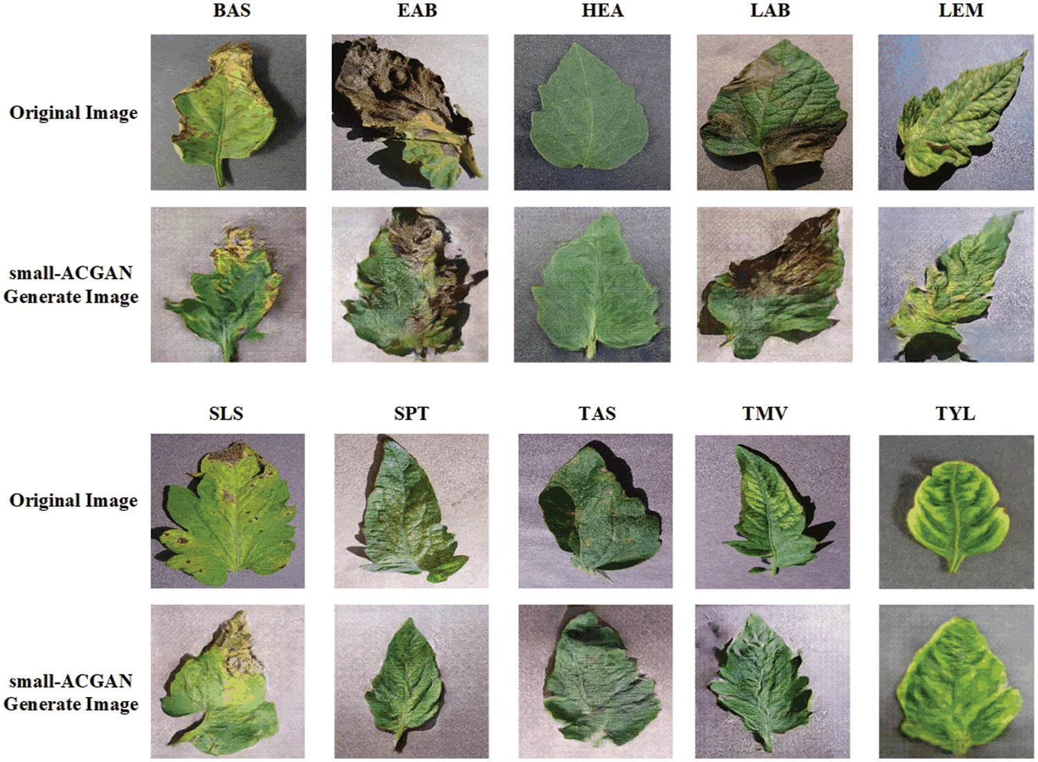
Figure 3: Comparison of original images and small-ACGAN generated images for each category: row 1 is the original image of five categories (Bacterial Spot, Early Blight, Healthy, Late Blight, Leaf Mold), row 2 is the corresponding generated image; row 3 is the original image of five categories (Septoria Leaf Spot, Two-spotted Spider Mite, Target Spot, Mosaic Virus, Yellow Leaf Curl Virus), row 4 is the corresponding generated image

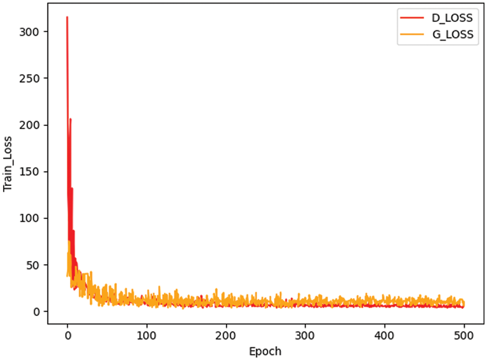
Figure 4: Generator and discriminator loss during training

4.4 Classification Model Performance

4.4.1 Expanded Dataset

In order to explore whether the number of images generated by small-ACGAN affects the performance of the classification model, this paper evaluates the performance of the classifier in four cases (0.25 times, 0.5 times, one time, and two times the extended data of the original training set).

Since the accuracy rate fluctuates during training, the images cannot be judged clearly. That is why using TensorBoard’s smoothing formula facilitates observing performance improvement in various cases, as shown in Eqs. (17) and (18). It is also noticeable from Fig. 5 that the performance of the network model during training is better for the doubled dataset than for the other datasets.

Px−new=(Px−1∗weight+Px)/(weight+1)(17)

weight=(weight+1)∗smooth(18)

where Px denotes the accuracy of the network at the x-th training; weight indicates the dynamic weight; smooth is the smoothing factor; and Px−new stands for the accuracy of the network at the x-th training after smoothing.

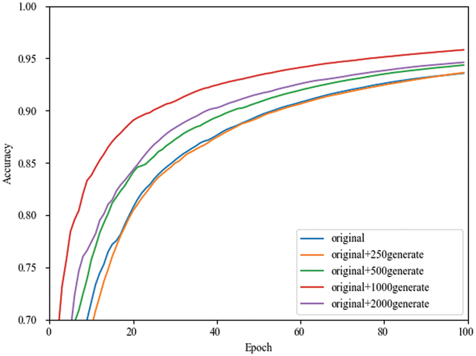
Figure 5: Smoothing curves of the validation set accuracy in MobileNetV3 network for different numbers of expanded datasets

Table 5 shows the effect of expanding the dataset with different multiples on the accuracy of the validation and test sets under the four CNN identification networks. Dataset original means 1000 images from the original dataset, 0.25 times means 1000 original images and 250 generated images, 0.5 times means 1000 original images and 500 generated images, one time means 1000 original images and 1000 generated images, and two times means 1000 original images and 2000 generated images.

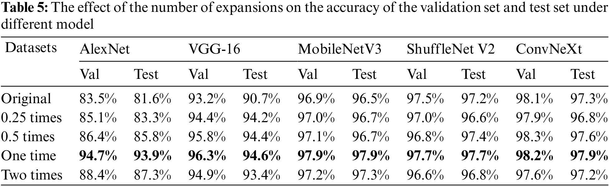
From Table 5, it can be concluded that among the four identification networks, the accuracy of both validation and test sets is the highest when doubling the dataset. Notably, the improvement is more evident for older networks, and there is also about 1% of progress in accuracy in newer networks. Based on the best results after doubling the expansions derived from the experiments in this chapter, this paper chose to double the expansions in the upcoming experiments.

4.4.2 Test Performance

The experiments in this section are mainly to verify the performance of the proposed method and the original and doubled images based on four CNN recognition models for evaluation. Their accuracy, precision, recall, and F1 scores are listed in the Table 6. As shown, compared to the original dataset, each metric improved by 12.23% on average for the AlexNet model, 3.77% for the VGG-16 model, 1.38% for the MobileNetV3 model, and 0.48% for the ShuffleNet V2 model. The fact that the F1 scores are higher than the original ones is also a good indication that small-ACGAN prevents the overfitting of the network and enhances the network model recognition ability.

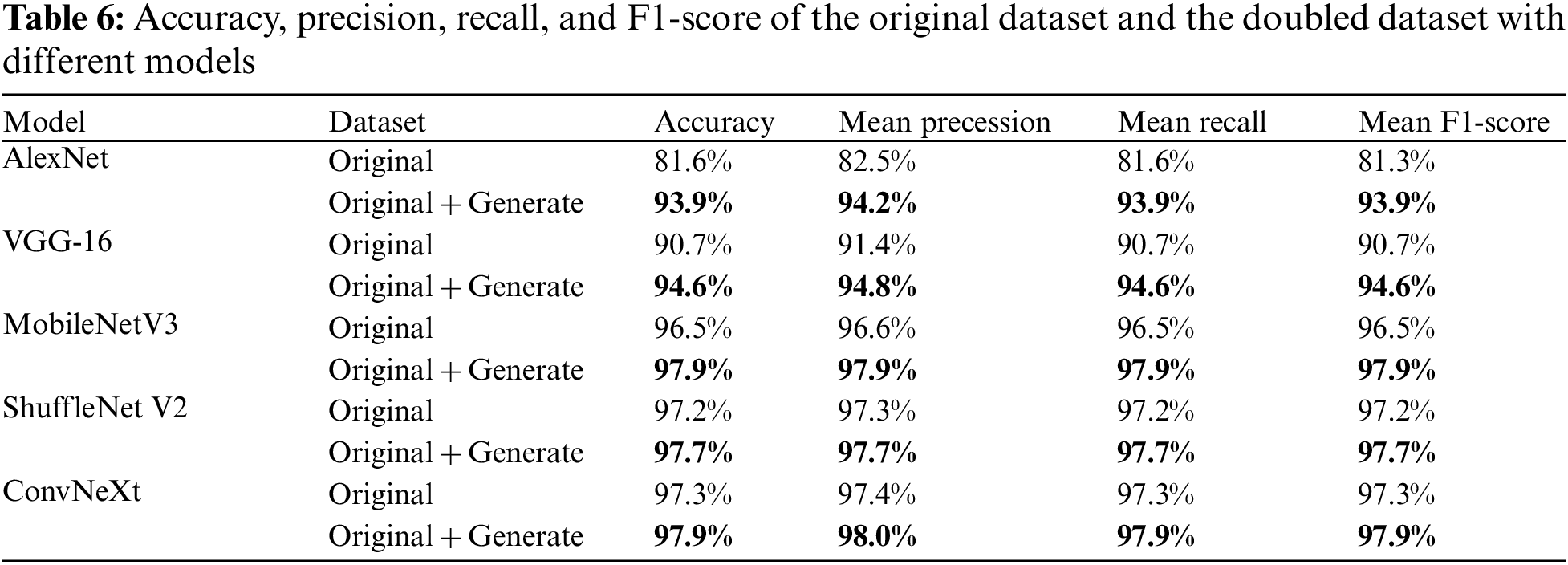
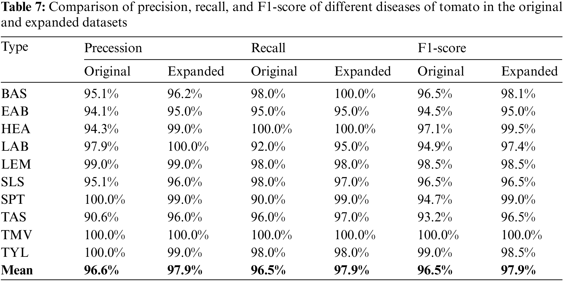
Table 7 compares the precision, recall, and F1 scores for different tomato diseases in the original and extended datasets. The data indicate that the scores of at least 8 of the ten leaf disease classes in the extended dataset are higher than the original ones, and the average values are all higher than the original ones, indicating that the method proposed in this paper is effective for each class of diseases.

Figs. 6 and 7 show the confusion matrix and ROC curves of the images generated by the proposed method in the MobileNetV3 model. In Fig. 6, most of the ten ROC curves lie in the upper left corner, and the AUC area is close to 1. In addition, from the comparison of the confusion matrix of the original dataset and the small-ACGAN dataset in Fig. 7, it can be seen that the proposed method in this paper produces very few false positives and false negatives.

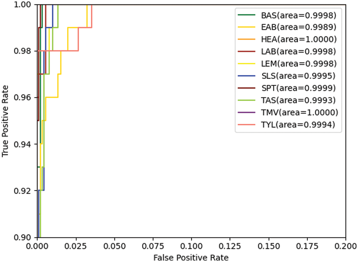
Figure 6: ROC curves based on the expanded dataset and MobileNetV3

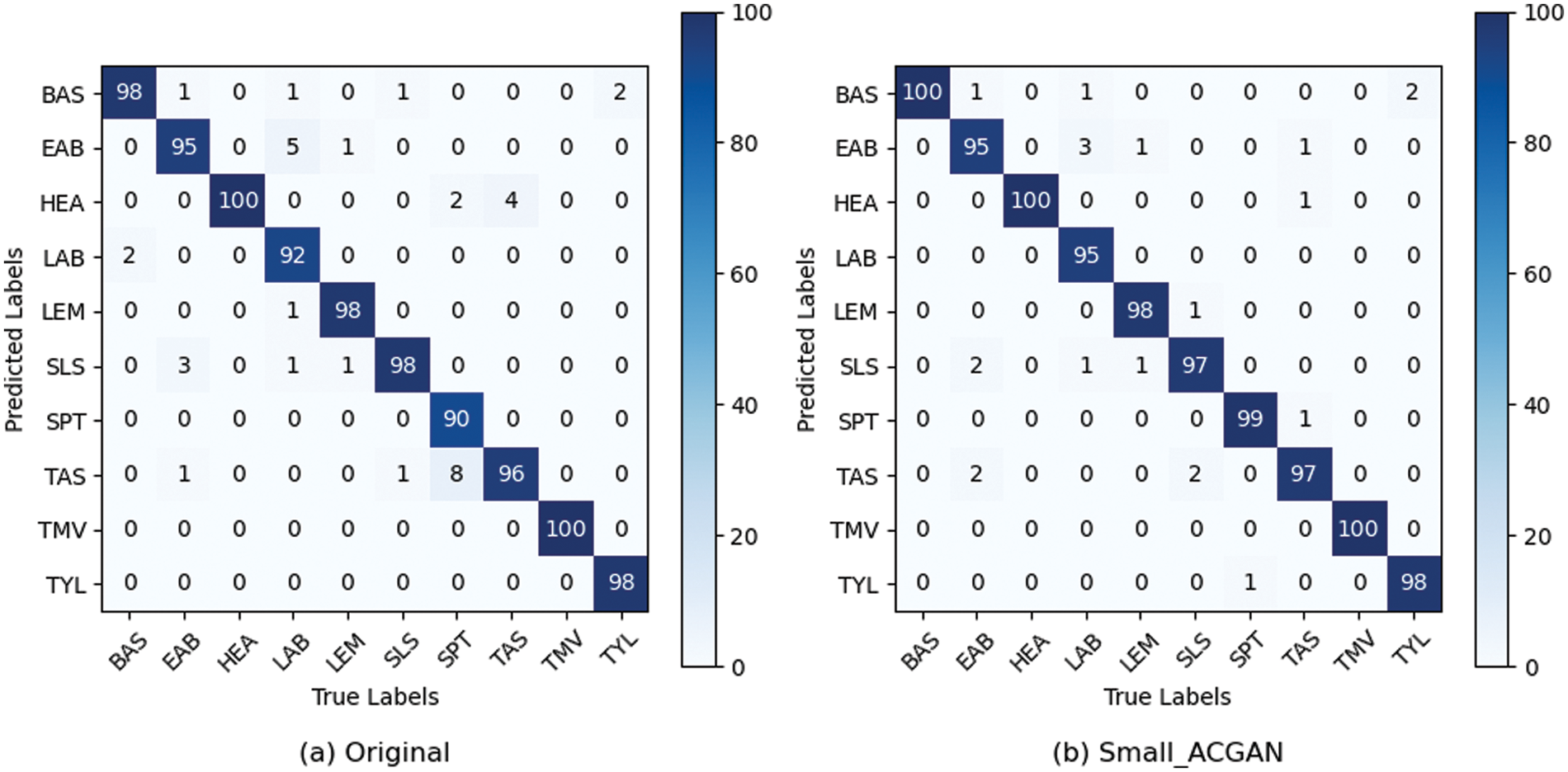
Figure 7: Confusion matrix based on the expanded dataset and MobileNetV3

4.5 Ablation Experiments

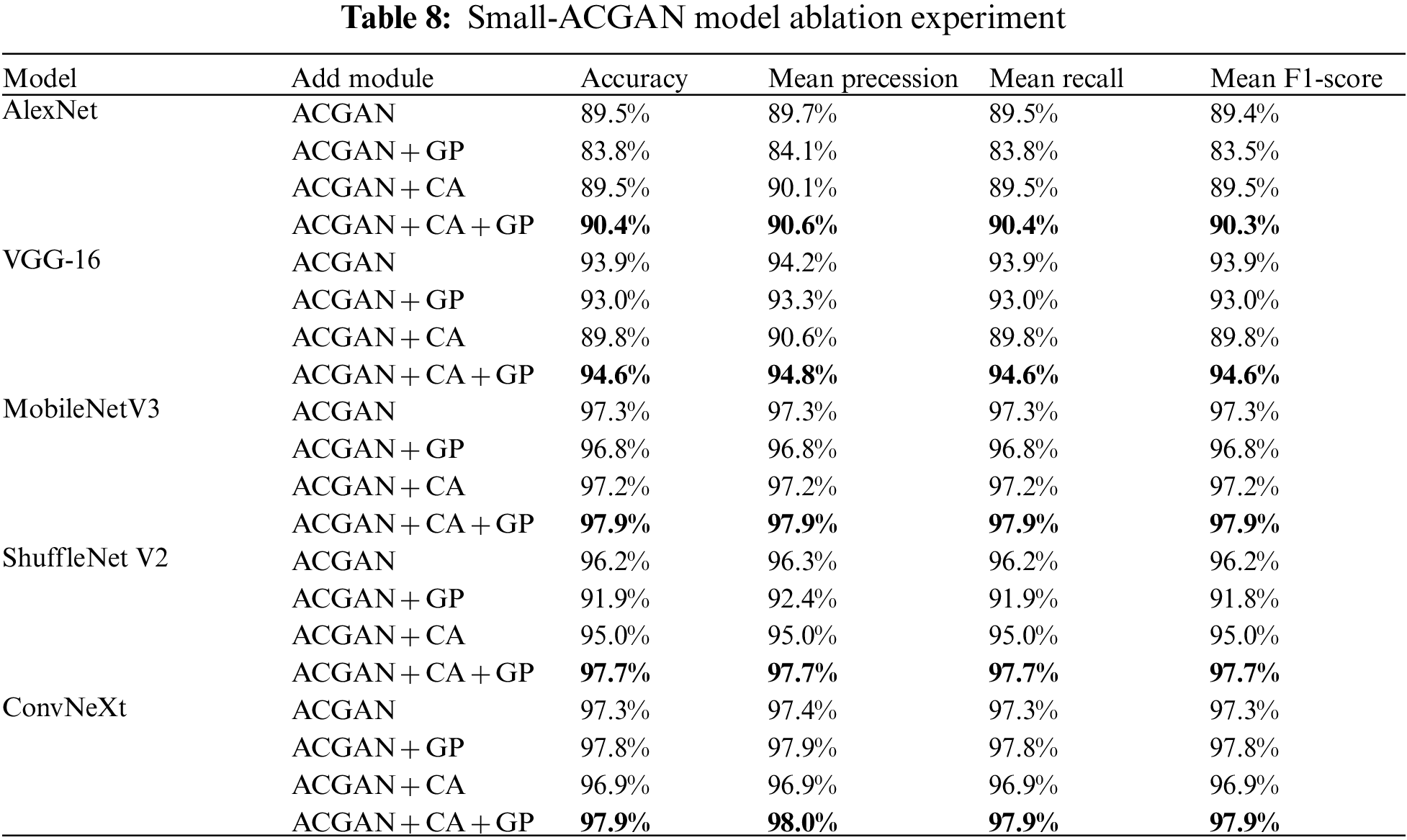
With a focus on improving the ACGAN model, this paper added CA to the ACGAN generator models and applied a gradient penalty mechanism to the discriminator loss while setting up ablation experiments to verify the effectiveness of the fused module. Experiments were conducted separately for ACGAN by adding CA and gradient penalty models. The results are suitable in Table 8, and ACGAN + CA + GP is the small-GAN in this paper. As can be seen from the table, the highest average Accuracy, average Precession, average Recall, and average F1-Score among the five CNN recognition networks is the ACGAN + CA + GP model, the lowest is ACGAN+GP, and the second to last is ACGAN + CA. The outcomes without adding but keeping the two models alone were not very effective; instead, the network model’s accuracy would reach the best level only when combined.

4.6 Comparison Experiments

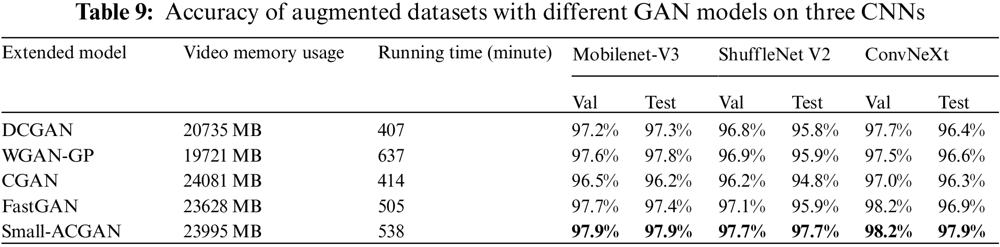
In order to evaluate the effectiveness of the proposed model, this paper compared small-ACGAN with several currently popular GANs. Table 9 indicates the results of these procedures, where the datasets produced by the proposed method outperform the datasets produced by the other GANs in the three CNN classification models. Although small-ACGAN and CGAN consume more video memory, they are convenient because they add classification information to the generator. DCGAN, WGAN-GP, and FastGAN can only be trained and generated one category at a time because they do not have classification information. While WGAN-GP and small-ACGAN take longer to run, mainly because these two GANs have a gradient penalty in the loss function, requiring additional time.

4.7 General Experiments

The experiments in this section choose grapes and apples [33] to verify the generality of small-ACGAN in data scaling. Both datasets have four classes, and each of the four CNN recognition networks was trained with 50 epochs, with other parameters referring to the Image Classification section in Table 4. As can be seen from Table 10, the results of both grape and apple datasets after the expansion using small-ACGAN were better than the original datasets, with an average 2% of improvement in accuracy under the four recognition networks in the grape dataset and an average of 4% of progress in the apple dataset. Fig. 8 illustrates the training accuracy smoothing curves for the original and expanded datasets of grapes under different models. The figure shows that the accuracy of the extended dataset is consistently higher than the original dataset during the training process. Consequently, this section concludes that small-ACGAN applies to the extension of other datasets.

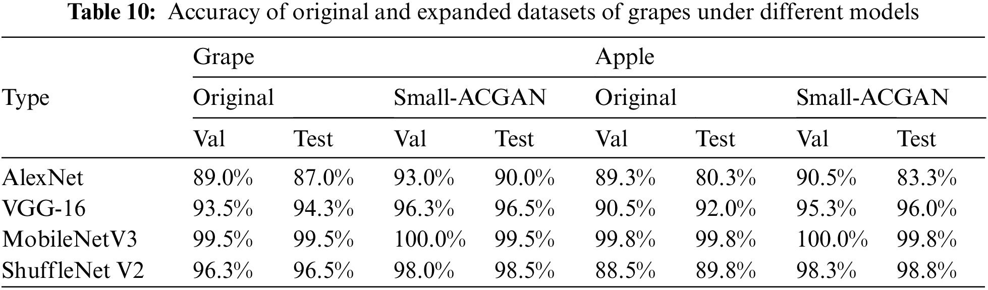
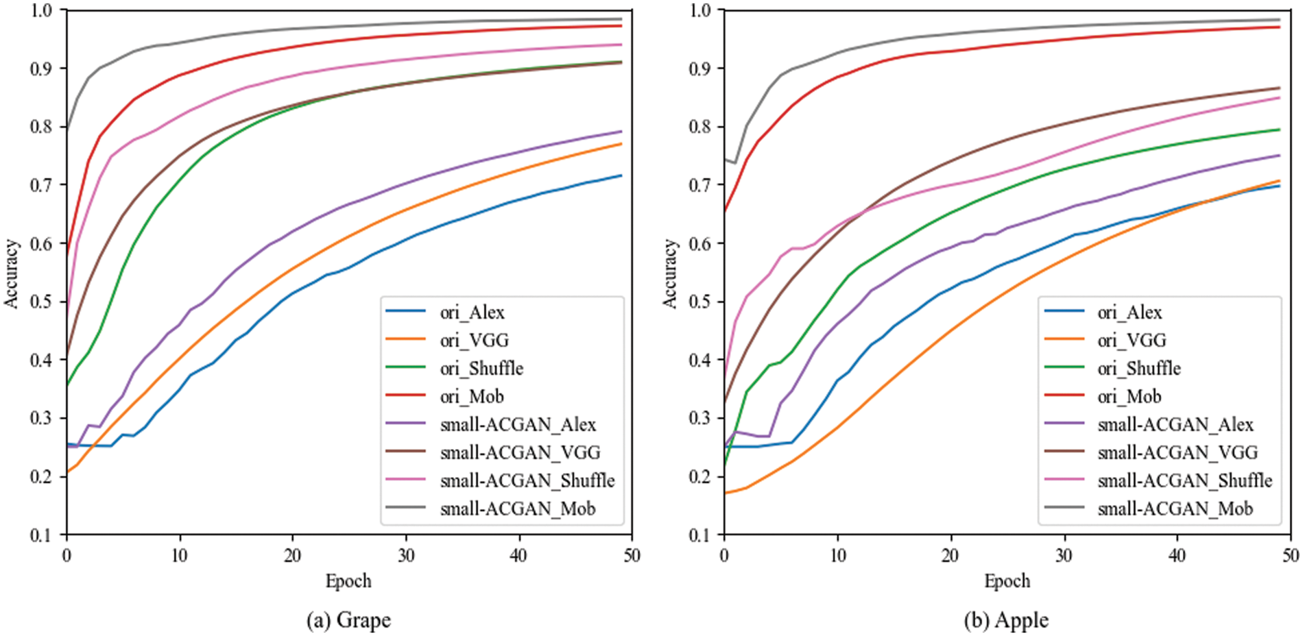
Figure 8: Training accuracy smoothing curves for original and expanded datasets of grapes under different models

5  Conclusion

This paper proposes a small ACGAN based on improving the ACGAN model used for plant disease identification in small samples. The main enhancements of this paper lie in two aspects: network structure and loss function. The experiments compare various attention mechanisms and incorporate CA into the generator of ACGAN to enhance image quality and highlight diseases. Furthermore, this paper adopts a gradient penalty to optimize the discriminator’s loss function for enhancing the training’s stability.

Following the contrast of the data with 0.25 times, 0.5 times, one time, and two times expansions, this paper observed that the best results resulted from doubling the expansion. In addition, the experimental accuracy, precision, recall, and F1-score of the five CNN classifiers on the enhanced dataset improved by an average of 3.74%, 3.48%, 3.74%, and 3.80% compared to the original dataset. In CNN classifier recognition, the dataset expanded by small-ACGAN achieves 94.2% accuracy on AlexNet, 94.8% on VGG-16%, 97.9% on ConvNeXt, 97.7% on ShuffleNet V2%, and 97.9% on MobileNetV3 with AUC close to 1, effectively improving the accuracy of CNN classifier recognition. Moreover, the overall performance of small-ACGAN was better than DCGAN, WGAN-GP, CGAN, and FastGAN.

However, the dataset used in this paper was pre-processed, so the results are pretty good. If the dataset is captured randomly, the generated results will be unsatisfactory. It is also challenging to create images with the current diseases for some datasets that are diseased but not diseased. Another point is that the training time of the method in this paper is slightly longer compared to the random cropping method.

In terms of further efforts, it is desirable to optimize the structure and related parameters of small-ACGAN to reduce the time spent on training and the utilization of video memory during training. There is also a desire to extend small-ACGAN to identify diseases in other parts of the plant, not only leaf diseases.

Acknowledgement: The authors are grateful to all members of the Zhejiang Provincial Key Laboratory of Forestry Intelligent Monitoring and Information Technology Research for their advice and assistance in the course of this research.

Funding Statement: The authors received no specific funding for this study.

Conflicts of Interest: The authors declare that they have no conflicts of interest to report regarding the present study.

References

1. Fao, FAO launches 2020 as the UN’s International Year of Plant Health. [online]. Available: https://www.fao.org/news/story/en/item/1253551/icode/ (Accessed 4.17, 2023). [Google Scholar]

2. Y. Liu, Y. Hu, W. Cai, G. Zhou and J. Zhan et al., “DCCAM-MRNet: Mixed residual connection network with dilated convolution and coordinate attention mechanism for tomato disease identification,” Computational Intelligence and Neuroscience, vol. 2022, pp. 1–15, 2022. [Google Scholar]

3. Y. Li, J. Nie and X. Chao, “Do we really need deep CNN for plant diseases identification?” Computers and Electronics in Agriculture, vol. 178, pp. 105803, 2020. [Google Scholar]

4. S. P. Mohanty, D. P. Hughes and M. Salathé, “Using deep learning for image-based plant disease detection,” Frontiers in Plant Science, vol. 7, pp. 1419, 2016. [Google Scholar] [PubMed]

5. C. Szegedy, W. Liu, Y. Jia, P. Sermanet and S. Reed et al., “Going deeper with convolutions,” in Proc. of the IEEE Conf. on Computer Vision and Pattern Recognition, Boston, Massachusetts, USA, pp. 1–9, 2015. [Google Scholar]

6. S. Ghosal and K. Sarkar, “Rice leaf diseases classification using CNN with transfer learning,” in 2020 IEEE Calcutta Conf. (CALCON), Kolkata, India, pp. 230–236, 2020. [Google Scholar]

7. K. Simonyan and A. Zisserman, “Very deep convolutional networks for large-scale image recognition,” arXiv preprint arXiv:1409.1556, 2014. [Google Scholar]

8. D. Jiang, F. Li, Y. Yang and S. Yu, “A tomato leaf diseases classification method based on deep learning,” in 2020 Chinese Control and Decision Conf. (CCDC), Hefei, China, pp. 1446–1450, 2020. [Google Scholar]

9. F. Zhong, Z. Chen, Y. Zhang and F. Xia, “Zero- and few-shot learning for diseases recognition of Citrus aurantium L. using conditional adversarial autoencoders,” Computers and Electronics in Agriculture, vol. 179, pp. 105828, 2020. [Google Scholar]

10. P. Pawara, E. Okafor, L. Schomaker and M. Wiering, “Data augmentation for plant classification,” in Advanced Concepts for Intelligent Vision Systems: 18th Int. Conf., Antwerp, Belgium, pp. 615–626, 2017. [Google Scholar]

11. A. Odena, C. Olah and J. Shlens, “Conditional image synthesis with auxiliary classifier gans,” in Proc. of the 34th Int. Conf. on Machine Learning, Sydney, Australia, pp. 2642–2651, 2017. [Google Scholar]

12. Q. Hou, D. Zhou and J. Feng, “Coordinate attention for efficient mobile network design,” arXiv preprint arXiv:2103.02907, 2021. [Google Scholar]

13. I. Goodfellow, J. Pouget-Abadie, M. Mirza, B. Xu and D. Warde-Farley et al., “Generative adversarial networks,” Communications of the Acm, vol. 63, no. 11, pp. 139–144, 2020. [Google Scholar]

14. A. Radford, L. Metz and S. Chintala, “Unsupervised representation learning with deep convolutional generative adversarial networks,” arXiv preprint arXiv:1511.06434, 2015. [Google Scholar]

15. I. Gulrajani, F. Ahmed, M. Arjovsky, V. Dumoulin and A. C. Courville, “Improved training of wasserstein gans,” Advances in Neural Information Processing Systems, vol. 30, pp. 5767–5777, 2017. [Google Scholar]

16. M. Mirza and S. Osindero, “Conditional generative adversarial nets,” arXiv preprint arXiv:1411.1784, 2014. [Google Scholar]

17. B. Liu, Y. Zhu, K. Song and A. Elgammal, “Towards faster and stabilized gan training for high-fidelity few-shot image synthesis,” in Int. Conf. on Learning Representations, Vienna, Austria, pp. 2101, 2021. [Google Scholar]

18. F. N. Al-Wesabi, A. Abdulrahman Albraikan, A. Mustafa Hilal, M. M. Eltahir and M. Ahmed Hamza et al., “Artificial intelligence enabled apple leaf disease classification for precision agriculture,” Computers, Materials & Continua, vol. 70, no. 3, pp. 6223–6238, 2022. [Google Scholar]

19. S. Sabour, N. Frosst and G. E. Hinton, “Dynamic routing between capsules,” Advances in Neural Information Processing Systems, vol. 30, pp. 3859–3869, 2017. [Google Scholar]

20. Y. Zheng, “Water wave optimization: A new nature-inspired metaheuristic,” Computers & Operations Research, vol. 55, pp. 1–11, 2015. [Google Scholar]

21. Z. Cui, R. Ke, Z. Pu and Y. Wang, “Stacked bidirectional and unidirectional LSTM recurrent neural network for forecasting network-wide traffic state with missing values,” Transportation Research Part C: Emerging Technologies, vol. 118, pp. 102674, 2020. [Google Scholar]

22. A. Elaraby, W. Hamdy and S. Alanazi, “Classification of citrus diseases using optimization deep learning approach,” Computational Intelligence and Neuroscience, vol. 2022, pp. 1–10, 2022. [Google Scholar]

23. Y. Wu and L. Xu, “Image generation of tomato leaf disease identification based on adversarial-VAE,” Agriculture, vol. 11, no. 10, pp. 9801, 2021. [Google Scholar]

24. F. Zhu, M. He and Z. Zheng, “Data augmentation using improved cDCGAN for plant vigor rating,” Computers and Electronics in Agriculture, vol. 175, pp. 105603, 2020. [Google Scholar]

25. B. Liu, C. Tan, S. Li, J. He and H. Wang, “A data augmentation method based on generative adversarial networks for grape leaf disease identification,” IEEE Access, vol. 8, pp. 102188–102198, 2020. [Google Scholar]

26. M. Heusel, H. Ramsauer, T. Unterthiner, B. Nessler and S. Hochreiter, “Gans trained by a two time-scale update rule converge to a local nash equilibrium,” Advances in Neural Information Processing Systems, vol. 30, pp. 6626–6637, 2017. [Google Scholar]

27. A. Abbas, S. Jain, M. Gour and S. Vankudothu, “Tomato plant disease detection using transfer learning with C-GAN synthetic images,” Computers and Electronics in Agriculture, vol. 187, pp. 106279, 2021. [Google Scholar]

28. G. Huang, Z. Liu, L. Van Der Maaten and K. Q. Weinberger, “Densely connected convolutional networks,” in Proc. of the IEEE Conf. on Computer Vision and Pattern Recognition, Hawaii, USA, pp. 4700–4708, 2017. [Google Scholar]

29. C. Zhou, Z. Zhang, S. Zhou, J. Xing and Q. Wu et al., “Grape leaf spot identification under limited samples by fine Grained-GAN,” IEEE Access, vol. 9, pp. 100480–100489, 2021. [Google Scholar]

30. S. Ren, K. He, R. Girshick and J. Sun, “Faster R-CNN: Towards real-time object detection with region proposal networks,” in Advances in Neural Information Processing Systems, Montreal, Canada, pp. 91–99, 2015. [Google Scholar]

31. Y. Zhang, S. Wa, L. Zhang and C. Lv, “Automatic plant disease detection based on tranvolution detection network with GAN modules using leaf images,” Frontiers in Plant Science, vol. 13, pp. 875693, 2022. [Google Scholar] [PubMed]

32. H. Zhang, I. Goodfellow, D. Metaxas and A. Odena, “Self-attention generative adversarial networks,” in Int. Conf. on Machine Learning, Lugano, Switzerland, pp. 7354–7363, 2019. [Google Scholar]

33. A. Ali, “PlantVillage dataset,” [online]. Available: https://www.kaggle.com/datasets/abdallahalidev/plantvillage-dataset (Accessed 1.12, 2023). [Google Scholar]

34. J. Hu, L. Shen and G. Sun, “Squeeze-and-excitation networks,” in Proc. of the IEEE Conf. on Computer Vision and Pattern Recognition, Salt Lake City, USA, pp. 7132–7141, 2018. [Google Scholar]

35. S. Woo, J. Park, J. Lee and I. S. Kweon, “Cbam: Convolutional block attention module,” in Proc. of the European Conf. on Computer Vision (ECCV), Munich, Germany, pp. 3–19, 2018. [Google Scholar]

36. N. Ma, X. Zhang, H. Zheng and J. Sun, “Shufflenet v2: Practical guidelines for efficient cnn architecture design,” in Proc. of the European Conf. on Computer Vision (ECCV), Munich, Germany, pp. 116–131, 2018. [Google Scholar]

37. A. Howard, M. Sandler, G. Chu, L. Chen and B. Chen et al., “Searching for mobilenetv3,” in Proc. of the IEEE/CVF Int. Conf. on Computer Vision, Seoul, Korea, pp. 1314–1324, 2019. [Google Scholar]

38. Z. Liu, H. Mao, C. Wu, C. Feichtenhofer and T. Darrell et al., “A convnet for the 2020s,” in Proc. of the IEEE/CVF Conf. on Computer Vision and Pattern Recognition, New Orleans, Louisiana, USA, pp. 11976–11986, 2022. [Google Scholar]

39. I. Sutskever, J. Martens, G. Dahl and G. Hinton, “On the importance of initialization and momentum in deep learning,” in Int. Conf. on Machine Learning, Atlanta, Georgia, USA, pp. 1139–1147, 2013. [Google Scholar]