An Improved Fully Automated Breast Cancer Detection and Classification System

1  Introduction

Recently, numerous models have been developed to distinguish and classify breast tumors [1–3]. These methods use various techniques to identify these tumors and are between 98.45% and 99.147% accurate. Unfortunately, many of these methods also take precious time to come to a diagnosis. Consequently, this study aims to develop a new method with reduced processing time, improved accuracy, and promising output.

A breast tumor is a tumor that arises when breast tissue grows unexpectedly. This uncontrollable growth occurs more often in women, though it affects men as well [1–5]. The World Health Organization (WHO) has declared breast cancer one of the most lethal diseases affecting women [3,6]. WHO reports that breast cancer causes more than 600,000 deaths yearly, which could be doubled later [1]. It is considered the leading cause of death among middle-aged women [5–8]. There is a vital need for a reliable and practical model to detect breast tumors early so that healthcare providers can prepare a plan for treatment and recovery [7,8]. Most developed models and utilized datasets categorized the disease as slow-grow (B) or aggressive (M). Hence, the presented algorithm classifies the detected masses into two types, B or M. Most of the symptoms appear in an advanced stage. Diagnosing this disease lately could lead to death as no treatments could cure it permanently [1,2,7,9,10]. Patients may see changes in the shape, size, and appearance of the breast from tumors. In addition, they may experience itching and tenderness at the tumor site [11–14]. In some cases, lumps on the breast occur due to infections which imply no tumors [1,2]. Physicians or pathologists use mammographic images to check whether tumors exist [1,15–22]. Cancer happens due to abnormal changes or uncontrollable growth in lobules or ducts tissues [23,24]. This development is noticed by the naked eye or a suitable device [1]. This technique is the most reliable tool.

This study presents a fully reliable model to diagnose the tumors using two deep-learning techniques and the KNN classifier. This model achieves higher results than others, as [1–5] have reached. The presented algorithm utilizes five datasets with more than 555,000 images of different modalities. Details of this system are in Section 3.

1.1 Research Problem and Motivations

Pathologists manually use their eyes to examine mammographic images to recognize breast cancers [1–3]. Using human eyes in such situations consumes much time and is undependable, especially in extensive health facilities [1]. Recently, some implemented models, such as those in [2–4], achieved less than 98.6% accuracy, whereas some algorithms reached nearly 98.9%, and the system in [1] achieved 99.147%. Consequently, there is a need and necessity to overcome this limitation by developing a fully automated, practical, reliable, and trustworthy model. This research presents a fully automatic approach to locating, detecting, and categorizing breast tumors. Since all datasets contain these types, this approach utilizes different modalities of Magnetic Resonance Imaging (MRI), mammographic, and histopathological images. The developed method classifies tumors as Benign Tumors (BT) or Malignant Tumors (MT) based on the extracted features, such as the radius of the detected tumors, texture, area, and smoothness. In total, 25 characteristics are utilized in this study.

Improving accuracy, reducing death rates, and saving lives by diagnosing breast cancers in their early stage are the motivations of this research. These motivations thrive the authors to conduct this study to propose an effective and practical model.

1.2 Research Contributions

The key contributions of this research are suggesting a consistent CAD method with reliable accuracy and deploying the KNN method to save lives and increase correctness by spotting tumors quickly. In addition, this research aims to reduce the execution time. These purposes inspired the authors to present a fully automated algorithm to discover and appropriately group tumors into their suitable types. This paper is structured as follows; Section 2 includes the related work on the considered disease. The presented model is explained intensively in Section 3. The findings and discussion are shown in Section 4. To conclude the conclusion is in Section 5.

2  Literature Review

Various studies have been conducted to diagnose breast cancer using different datasets. These studies developed different methods discussed in this section.

Alsheikhy et al. in [1] presented a system to detect and group breast tumors using AlexNet and three classifiers. The authors utilized mammographic images, and AlexNet was deployed to perform the algorithm’s deep learning phase. Three datasets from Kaggle were used to train the algorithm. This approach achieved 99.147% accuracy on the testing dataset. It classified the tumors it recognized as benign or malignant. Various image preprocessing approaches were employed to that effect. Several performance metrics were computed to evaluate the implemented model. The authors achieved 99.687% precision, 99.407% recall, 94.871% specificity, and a 99.547% F-score. In [1], the developed system used the fuzzy c-mean technique, the KNN, the Decision Tree, and the Bayes algorithms to detect and classify cancers as benign or malignant. They tested 3400 mammographic images, and every input’s processing time was between 3 and 4.87 s.

The presented method, in contrast to [1], uses two deep learning tools rather than one, namely ResNet50 and AlexNet. These tools were customized and integrated with the KNN algorithm to diagnose and classify breast tumors as Benign Tumors (BT) or Malignant Tumors (MT) because all five datasets utilized categorized cancers as B or M. The presented model was trained with over 60,000 mammographic images and tested on a dataset of 12,000 images. All images were different sizes, and the presented algorithm was able to resize those inputs to be readable by the customized ResNet50 and AlexNet tools. The proposed method achieved 99.38% accuracy. It achieved 99.71% precision, 99.46% recall, 98.08% specificity, and an F-score of 99.67 outperforming the implemented model in [1] by every measurement.

In [2], Akkur et al. presented a novel classification model utilizing machine learning algorithms to diagnose breast cancers in their early stage. This model used feature selection and Bayesian optimization algorithms. Numerous machine learning techniques were applied to two datasets: a Support Vector Machine (SVM), the KNN, the Naive Bayes, Ensemble Learning, and the Decision Tree. These datasets were Wisconsin Breast Cancer Dataset (WBCD) and Mammographic Breast Cancer Dataset (MBCD). The authors utilized the Least Absolute Shrinkage and Selection Operator (LASSO) to determine the most relevant features. The implemented model achieved 97.95%, 98.28%, 98.28%, and 98.28% for accuracy, precision, recall, and F-score, respectively, for both datasets. 764 images were used. In contrast, the proposed method utilized around 72,000 pictures and obtained 99.38%, 99.71%, 99.46%, 98.08%, and 99.67% for all considered performance quantities, respectively, on five datasets. Moreover, two deep learning tools and the KNN algorithm were integrated and customized to reach the highest accuracy. The presented model outstands the method in [2].

Umer et al. in [3] developed a framework to identify breast tumors using deep learning and selection based on histopathological images. Nearly 277,000 images were used. The method deployed three steps: deep learning to extract features, a novel features selection framework that took inputs from the deep learning tool, and use of machine learning algorithms to classify data into two groups: normal and invasive ductal carcinoma. The authors of [3] achieved 92.7% accuracy in their diagnoses. The model they developed also had 87% precision and sensitivity. The presented method in our study utilized 72,000 images and deployed two deep learning tools and the KNN approach to achieve 99.38% accuracy in diagnosis.

Drinkovic et al. in [4] performed a comparative accuracy evaluation between two protocols. These protocols were a modified innovative abbreviated MRI protocol (AMRP) and a standard magnetic resonance protocol (SMRP) to diagnose the disease. This evaluation was conducted on 477 patients using MRI images. 232 patients out of 477 were assigned to AMRP, while the rest were given to SMRP. Those patients performed a core biopsy and a histopathological analysis. The ages of the patients were amidst 13 and 54. The authors declared that their evaluation yielded no significant difference between both protocols regarding specificity and sensitivity. The AMRP protocol yielded 99.05% sensitivity and 59.09% specificity, while another protocol achieved 98.12% and 68.75% for both metrics. The authors provided no information about their obtained accuracy. In contrast, the proposed method was trained and tested on more than 70,000 images using two deep-learning tools and the KNN technique to accurately identify and classify breast tumors. This method achieved 99.38% accuracy, while its specificity and sensitivity values were 98.08% and 99.46%, respectively. These results indicate that the presented model is better than the method in [4] and produces exquisite findings.

In [8], Wang et al. developed a method to diagnose the tumors inside the breast using four datasets to train their algorithm. The authors compared their approach with 13 deep-learning tools. The method developed reached 87.77% accurate diagnoses on the first dataset, 94.64% on the second dataset, and 93.54% on the third dataset on less than 140 images. The low accuracy rate is expected with the small sample size. The authors measured the success of their algorithm using four performance metrics: precision, accuracy, F-score, and accuracy. In comparison, this proposed method uses five metrics, as stated earlier. The authors in [8] accomplished 91.99% average accuracy. In contrast, the presented approach reached 99.38% average accuracy for all five datasets used in testing. The proposed method achieved 99.74% maximum accuracy.

Adebiyi et al. in [25] also implemented a computer-based model to enhance the process of breast cancer diagnosis, testing two machine learning techniques on the Wisconsin Breast Cancer Dataset (WBCD). The authors aimed to investigate breast cancer identification accuracy using two well-known machine learning tools: a Random Forest (RF) algorithm, and a Support Vector Machine (SVM) technique. A feature extraction tool of Linear Discriminant Analysis (LDA) was also used. The model achieved 96.4% accuracy for RF with LDA and SVM with LDA, respectively. In addition, when using RF with LDA, the authors attained 97% precision, 95.6% recall, 95.7% specificity, and a F-score of 96.3%. When they used SVM with LDA, they achieved 96.4%, 95.7%, 97.8%, and 97.8% on the same parameters. The presented CAD model achieves 99.38% accuracy, in contrast, using five datasets with different modalities, while the implemented model in [25] used only one dataset with no images and only written data.

In [26], the authors deployed a Particle Swarm Optimization (PSO) algorithm on a dataset from the University of California Irvine to select relevant features and extract them. This enabled them to classify tumors using an Artificial Neural Network (ANN) technique. The authors reached 97.13% accuracy in their diagnoses. The presented algorithm achieved 99.38% using two deep-learning techniques rather than one.

Afolayan et al. in [27] created a similar technology and suggested using a PSO algorithm with a Decision Tree tool to optimize the classification efficiency of breast tumors using WBCD. The authors reached 92.26% accuracy with this method. The proposed method is 7.164% higher accuracy. These numbers indicate that the given CAD system is better and more helpful for identifying and categorizing breast tumors with different technologies.

In [28], the authors presented a lymphocyte analysis framework technique that deployed a CNN to analyze histology images to identify lymphocytes. This framework contained four steps: preprocessing, scanning, localization, and postprocessing. Identification was conducted using a patch-level procedure. The required features were extracted from data using a dilated convolutional network, an attention mechanism, and a pyramid network. The authors used one dataset, NuClick, to evaluate their method, and achieved 84% and 83% for F-score and precision, respectively. When the authors participated in an open public challenge, the tool measured 76% and 73% for accuracy and F-score, respectively. The presented system uses two Deep Convolutional Neural Network (DCNN) tools to extract the mandatory characteristics from inputs, identify the tumor masses, and categorize these masses accordingly. In contrast, the proposed system used five datasets with different modalities to evaluate the performance in terms of accuracy and other considered quantities. The presented model achieved 99.38% accuracy, outperforming the implemented method in [28] while building on its use of a multistep framework.

Table 1 lists a comparative evaluation of the utilized techniques, achieved results, advantages, and disadvantages of existing approaches to AI-based breast cancer diagnosis tools.

3  The Proposed Algorithm

3.1 Problem Statement

The recently published articles on breast cancer identification and classification, such as those in [1–8], emphasize the importance of diagnosing and labeling tumors quickly and accurately. The authors in [1] attained an average accuracy of 99.147%, with a maximum obtained accuracy of 99.28%. Those authors deployed AlexNet and the Fuzzy C-Means clustering method. In addition, the developed model in [1] computed the values of the remaining performance quantities between 94.871% and 99.687%. Every implemented model in [1,2,4,5,8] took more processing time than anticipated. From a timing point of view, this elongated processing time is a disadvantage. With cancer, every moment counts. Results should be obtained in real-time. Consequently, this study aims to construct and implement a practical, consistent, and reliable method to diagnose and classify breast tumors precisely, correctly, and instantaneously while accomplishing a higher accuracy than preexisting technologies.

3.2 Deep Convolutional Neural Networks (DCNNs)

3.2.1 AlexNet

Various fields, including medicine, education, commerce, and industry, utilize Computer Vision (CV) and Artificial Intelligence (AI) technologies to improve the procedures and outcomes of their associated technologies [1–3]. Specifically, DCNNs have the demonstrated ability to support tracking, detecting, and categorizing objects in a multitude of fields efficiently and with low labor costs. In 2012, two researchers developed AlexNet, a new type of DCNN. Fig. 1 illustrates a general block diagram of AlexNet. This block diagram encompasses ten layers.

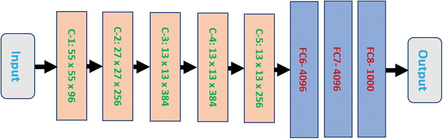
Figure 1: The general block diagram of the AlexNet structure

The block diagram has eight blocks between the first and the last layers. These blocks make up five convolutional layers and three fully connected layers. Each convolutional block is denoted as C-Y, where Y is broken down in ascending order from one to five. Each fully connected layer is characterized as FCX. X refers to the order number from six to eight. Each convolutional block contains its size, while every Fully Connected (FC) layer has a limited number of neurons it can hold.

3.2.2 ResNet 50

ResNet50 stands for Residual Network. It was first implemented in 2015 and is another form of a DCNN. ResNet50, as the name suggests, is comprised of 50 layers. The tool accepts an input size of 224 × 224. Fig. 2 illustrates a general block diagram of ResNet50.

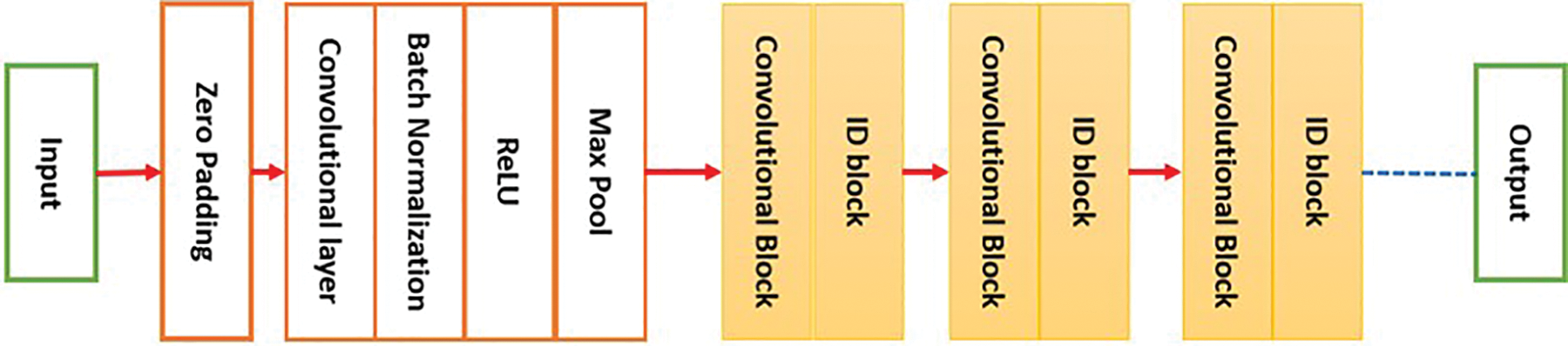
Figure 2: The block diagram of ResNet50

3.3 Datasets

This study utilizes five datasets: four are downloaded from Kaggle, and the remaining one is downloaded from a private site that requires registration and permission to download. These datasets are BreakHis v1 [29], KAU-BCMD [30], MIAS, Breast Histopathology Images (BHI), and BreCaHAD [31]. The dataset BreakHis v1 is almost 4.2 GB, with 7909 images. The images captured 2480 Benign tumors and 5429 Malignant. The second dataset, KAU-BCMD, is 593 MB, with more than 5500 images collected from 2019 to 2020. Among these images are 2717 Benign tumors and 2945 Malignant. The third dataset, MIAS, is 320 MB and contains 322 images. The fourth dataset is 3.1 GB and includes 555,000 images. The fifth dataset is approximately 1 GB and includes 162 images. These five datasets are utilized in the proposed method to train and test the algorithm. Specifically, 60,000 images from the BHI dataset were used for training, while more than 12,000 images from the remaining datasets were used to test and evaluate the model. The number of total extracted features is 25. Table 2 summarizes the properties of each used dataset, including the number of images, ground truth, modality, and dataset type.

3.4 The Proposed Methodology

In the first stage, five datasets are employed to assess and measure the proposed method’s ability to diagnose and classify breast cancer on multiple metrics. All five datasets contain different modalities, as shown in Table 2. All images across datasets were classified as Healthy, Benign Tumors (BT), and Malignant Tumors (MT). The datasets were divided into two groups during the study: 60,000 images were allocated as the training set, and nearly 12,000 images comprised a testing set. The training and testing processes took approximately 13 h.

The output of this study is an Improved, Fully Automated Breast Cancer Identification and Categorization System (IFABCICS) that deploys various image preprocessing techniques, two DCNNs, and the KNN algorithm. The KNN classification algorithm was utilized to classify prospective segmented areas of interest (PoI), or segmented tissues, into either normal or infected tissues. Infected tissues are classified (BT) or (MT).

In the second stage, called the preprocessing stage, numerous procedures and operations are performed, such as background removal, denoising, rescaling, resampling, and intensity normalization, to rescale inputs according to the needs of each utilized DCNN, eliminate noise, and improve the resolution of the inputs, segment images, and transform images to grayscale illustrations. Morphological, mask, Otsu, Discrete Wavelet Transform (DWT), and Principal Component Analysis (PCA) techniques are also applied to attain accurate outputs. Furthermore, Gabor and Laplace’s filters are used. Image segmentation is performed to find a potential area of interest where tumors are likely to be detected. DWT is used to remove noise from the images. Reducing the dimension size of inputs is achieved using the PCA tool; in this research, the achieved dimensional size is 8 × 8.

The next step is to use the KNN algorithm to cluster data into classes: Class 1 and Class 2. Class 1 denotes normal/healthy tissue, while Class 2 represents infected tissue. Class 2 is further classified into BT or MT groups. After that, the grouped data is sent to the DCNNs to start the training process. The KNN algorithm determines the center point for each class and denotes them with an X. The KNN approach runs more than 500 iterations in the training stage to reach maximum accuracy. The training lasts 11 h and obtains characteristic data from 60,000 images, including but not limited to radius, area, texture, and diameter. In total, 1,500,000 characteristics were generated from all inputs in this study. Then, the necessary features enter the categorization stage to label the tumors: benign cancer (BC) and malignant cancer (MC). BC and MC are the same as BT and MT, respectively.

Next, a confusion matrix is generated to show how the presented method classifies tumors into their classes. The obtained outputs are assessed through a comparison procedure with other developed approaches from the related work to determine how its outcomes compare to others.

Fig. 3 depicts a flowchart of the proposed method. This flowchart demonstrates how the presented method propagates data from one stage into another.

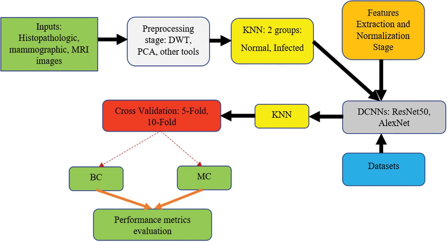
Figure 3: The flowchart of the proposed system

The input and outputs are colored green; the preprocessing stage is colored light gray; the clustering procedures are distinguished in yellow; the feature extraction and normalization phase are colored orange; the deep learning stage is colored dark gray, the datasets are represented in blue, and the cross-validation using the 5-Fold and the 10-Fold sets are shown in red. The second KNN method is used to classify the infected tissues into either (BC) or (MC).

In this study, 5-Fold and 10-Fold Cross-Validations are conducted. Table 3 illustrates how the 5-Fold scheme works.

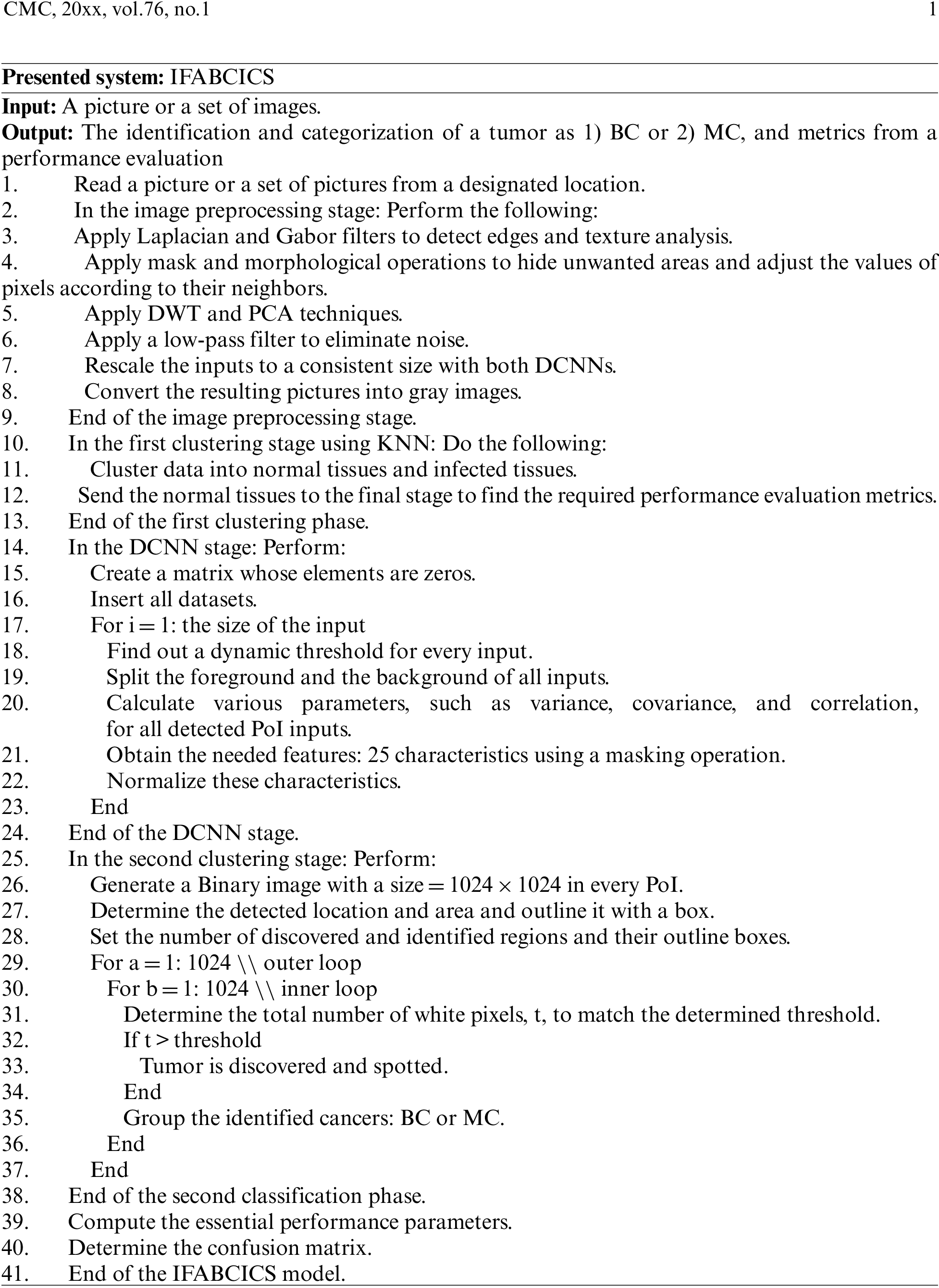
The following pseudo-codes demonstrate how the proposed system is implemented:

Various advantages can be achieved using this method, encapsulated as follows:

A.   The average achieved accuracy is 99.38%, while the maximum reached is 99.74%.

B.   The implemented method works on different modalities.

C.   The proposed method is fully automated.

D.   The algorithm is reliable and stable.

E.   No human intervention is required.

F.   The execution time, or the processing time, is between 2.4 and 3.9 s for each image.

G.   The presented method surpasses other implemented models mentioned in the related work section in all evaluated parameters listed below.

Multiple performance parameters, also referred to as metrics, are evaluated in the presented method, and these parameters are as follows:

1.    True Positive (TP).

2.    False Positive (FP).

3.    True Negative (TN).

4.    False Negative (FN).

5.    Precision (Pr) is computed via Eq. (1):

Pr=TP(TP+FP)(1)

6.    Recall (Rc), also known as sensitivity, is calculated via Eq. (2):

Rc=TP(TP+FN)(2)

7.    Accuracy (Ac) is determined via Eq. (3):

Ac=(TP+TN)(TP+TN+FP+FN)(3)

8.    Specificity (Sp): is computed via Eq. (4):

Sp=TN(TN+FP)(4)

9.    F-score is determined via Eq. (5):

F−Score=2×(Pr×Rc)(Pr+Rc)(5)

4  Results and Discussion

Various evaluation and validation experiments were performed in MATLAB R2017b to verify and test the presented method’s procedures and conclusions. The developed method was assessed over 10,000 times and ran for 13 h to train datasets to reach accurate findings. In the training stage, the for-loop command inside the presented method was constructed to run 15,000 times to let the model learn profoundly and intensely to accomplish reliable outputs. This step is important as two deep learning tools are involved. Multiple scenarios were examined and analyzed to explain and characterize how the proposed method works and propagates outputs to classify breast tumors. The computation of the necessary parameters, quantities, and confusion matrix are provided. A comparative evaluation between the presented model and some developed models is also included.

MATLAB was utilized in all tests because it can handle large amounts of data. It contains various built-in functions and toolboxes to process different types of images. A hosting machine with Windows 11 Pro was used with an Intel Core i7 8th generation central processing unit with 1.8 GHz speed and 16 GB RAM. In this study, two learning rates were utilized: L1 = 0.01 and L2 = 0.0001. L1 was applied to the 5-Fold scheme, while the 10-Fold method used L2.

The evaluated performance parameters are conducted based on quantitative and qualitative quantities. Almost all developed models measured their performance based on these parameters, while a few implemented algorithms computed fewer metrics. Accuracy remains the most critical metric and was measured for all methods. In this study, nearly 12,000 images with different modalities were tested and investigated, and 60,000 images were used for training. The sizes of the testing dataset images were rescaled to be readable by the two used deep learning tools. During the testing stage, an average value for every metric was determined after all images were scanned. The testing dataset required 164 min of processing time, and the proposed method ran for around 7,500 iterations.

Initially, the proposed method reached an average accuracy of 93.71% when 1,300 iterations were run with the 5-Fold scheme. The average accuracy was 91.45% for the 10-Fold scheme. These two values improved significantly when iterations were increased. The obtained average values for the considered performance quantities, namely accuracy, precision, sensitivity, specificity, and F-score, were 92.58%, 92.71%, 93.01%, 92.68%, and 94.13%, respectively, at the end of the Fold-1 stage. At the end of the Fold-5 scheme, the average values of all performance metrics increased by nearly 5.28%, as illustrated in Fig. 4.

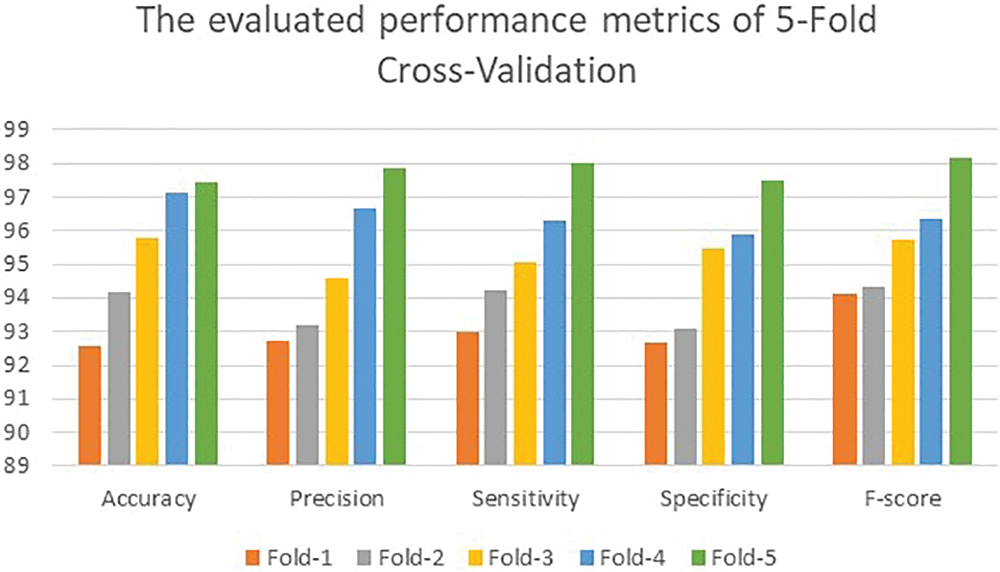
Figure 4: The achieved results of the 5-fold scenario

Fig. 5 depicts the obtained values of the considered performance metrics of the 10-Fold method.

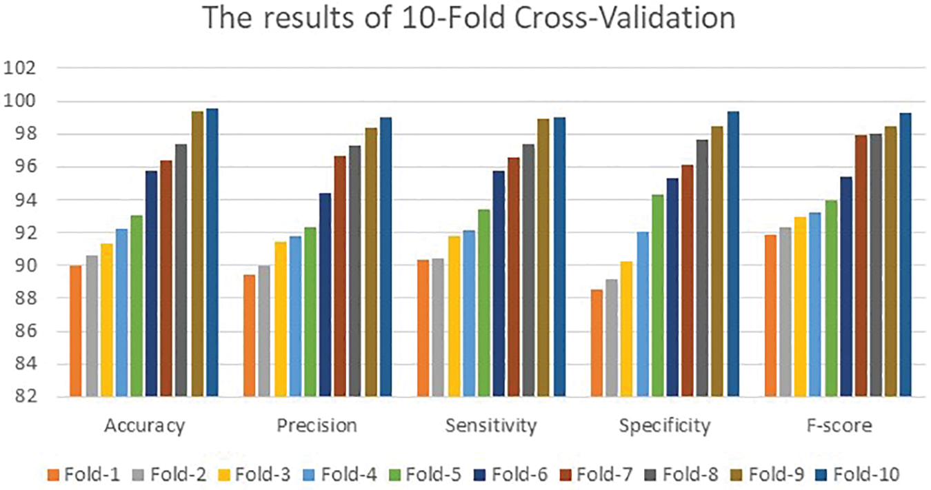
Figure 5: The determining outcomes of the 10-fold cross-validation technique

Fig. 5 also shows that the presented algorithm achieved 90.02%, 89.43%, 90.31%, 88.57%, and 91.86% for the performance metrics in the first fold. The presented algorithm achieved a maximum accuracy of 99.64% and a 99.83% F-score. These two values are higher than what other implemented models have reached. Both Figs. 4 and 5 show that all performance parameters improved after each fold. This improvement reaches its highest values after 3,476 iterations for 5-Fold Cross-Validations and 7,801 iterations of the 10-Fold Cross-Validation. This gap occurs due to the utilized values of the learning rates. The 5-Fold Cross-Validation stage reached its maximum accuracy value at 99.64%. The 10-Fold Cross-Validation part achieved maximum accuracy of 99.51% after more iterations suggesting that the proposed model converges slowly to its highest value due to the small value of the learning rate. The other examined performance metrics follow the same concept illustrated in Fig. 4. Fig. 5 reveals that the developed method accomplished better outcomes than in Fig. 4 since the method learns intensively from the number of iterations utilized.

This study examined 12,000 images with different modalities after the testing stage. Table 4 lists the maximum evaluated performance parameters of the proposed method for the 5-Fold and 10-Fold schemes. All values are given in percentages. The utilized testing dataset has 4,879 confirmed benign cases, 6,213 confirmed aggressive cases, and 908 healthy subjects. The average time spent on every image is between 2.47 to 3.89 s. This difference in the processing times was affected by the tested image’s types and the total number of required extracted features: all images contain 300,000 characteristics. Moreover, the detected tumors’ location, size, area, diameter, and correlation also play significant roles in processing time. All values were obtained after the technology ran 10,000 iterations.

Fig. 6 offers a graphical representation of all considered performance metrics in Table 4.

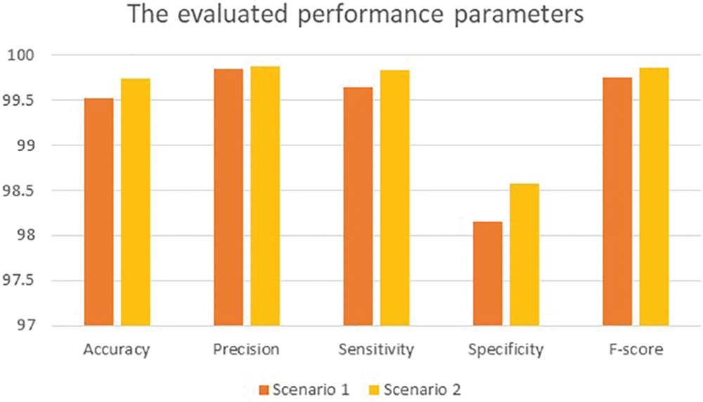
Figure 6: Graphical representation of the obtained results

For simplicity, the 5-Fold scheme is denoted as Scenario 1, while the 10-Fold scheme is represented as Scenario 2. The 10-Fold scheme yields better results, as shown in Fig. 6. The presented model achieved 99.20% accuracy when it deployed L1 and reached 97.7% accuracy when L2 = 0.0001. For the learning rate L1, there were 930 utilized iterations, with 30 epochs used. For the learning rate L2, 2,542 iterations were employed, with 82 epochs used as well. Every epoch for both L1 and L2 included 31 iterations. For both learning rates, 10 and 16 were the minimum and maximum batch sizes. In Scenario 1, the obtained accuracy approaches almost 100% after five epochs and becomes increasingly constant and steady. The loss function reaches zero after five epochs as it moves towards its steady state. The processing time is dependent on the batch sizes: processing a bigger batch size takes a longer time. In Scenario 2, diagnosis and classification took more time since the learning rate was lower. Table 5 shows the proposed method’s classification results for the 12,000 images. Excepting those images classified as Healthy (HB), images are classified as Benign Tumors (BT) and Malignant Tumors (MT). Table 5 lists the values of both for the 10-Fold Cross-Validation. Table 6 demonstrates the presented method’s confusion matrix of the obtained outcomes. Green refers to the adequately recognized and classified classes, while red denotes the improperly identified types.

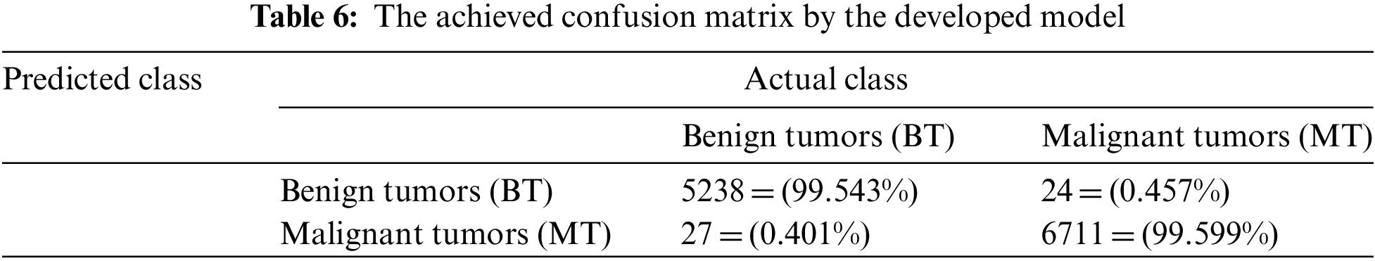
Table 6 shows that the presented model correctly identified and classified 5,238 BT samples out of 5,262 total benign images resulting in 99.543% accuracy. In addition, the implemented algorithm recognized precisely 6,711 MT inputs out of 6,738. The total number of inaccurately classified tumors came to 51 cases of 12,000 samples, which can be categorized as minimal and can be neglected.

Table 7 offers the comparative evaluation between the presented method and some implemented models from the literature. The compared works are [1–4] and [8,12,32,33]. This comparative assessment was based on the methodologies/techniques of each model and five performance parameters. N.I. stands for no information provided. The presented method in this study surpasses all other models in all considered metrics. The developed algorithm achieves the highest values and yields the best results among all compared works.

Fig. 7 illustrates the comparative assessment analysis of accuracy and F-score between the presented method and some recent algorithms.

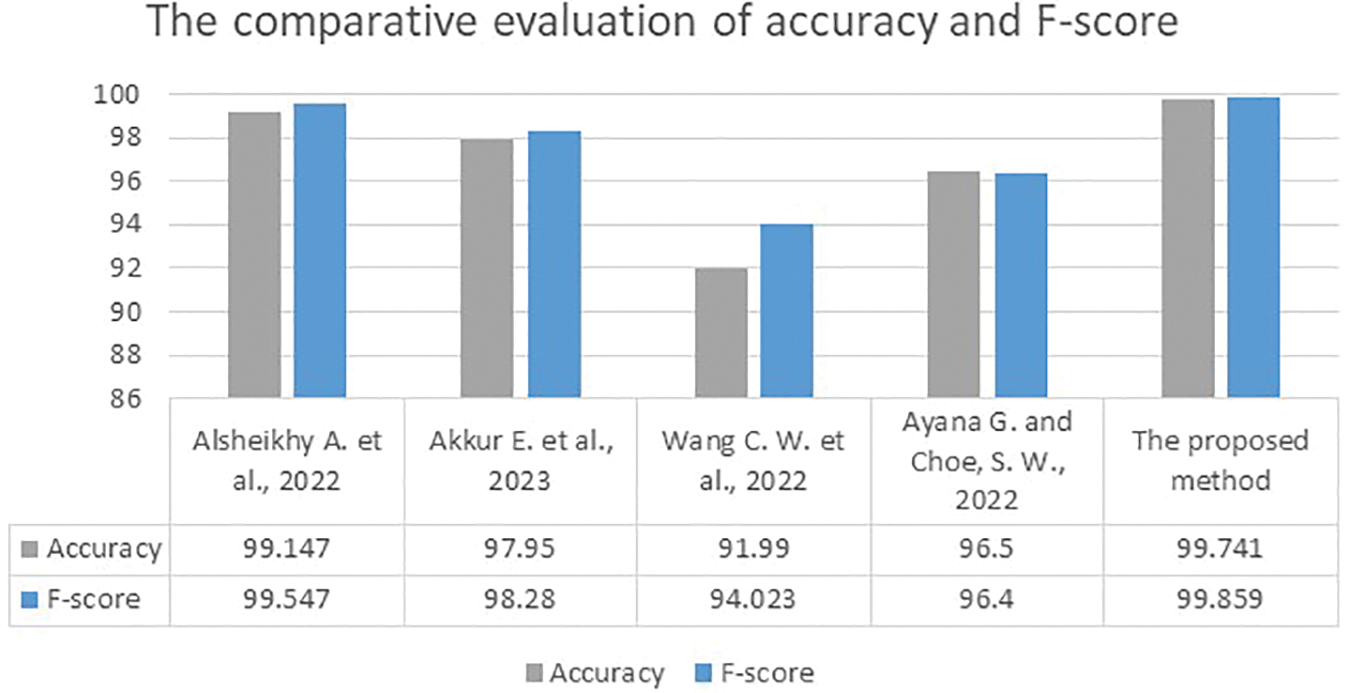
Figure 7: The comparative assessment of accuracy and F-score results between the presented approach and the developed works in [1,2,8,12]

The implemented work in [4] yielded the lowest accuracy and F-score values, while the implemented methods in [2,12] reached moderate accuracy and F-scores between 96.4% and 98.28%. The developed system in [1] achieved the highest values for accuracy and F-score: 99.147% in accuracy and a 99.547% F-Score. Surpassing even this method, the presented approach attained 99.7% accuracy and a 99.85% F-score. Figs. 8–10 depict samples of the obtained outputs of the proposed model.

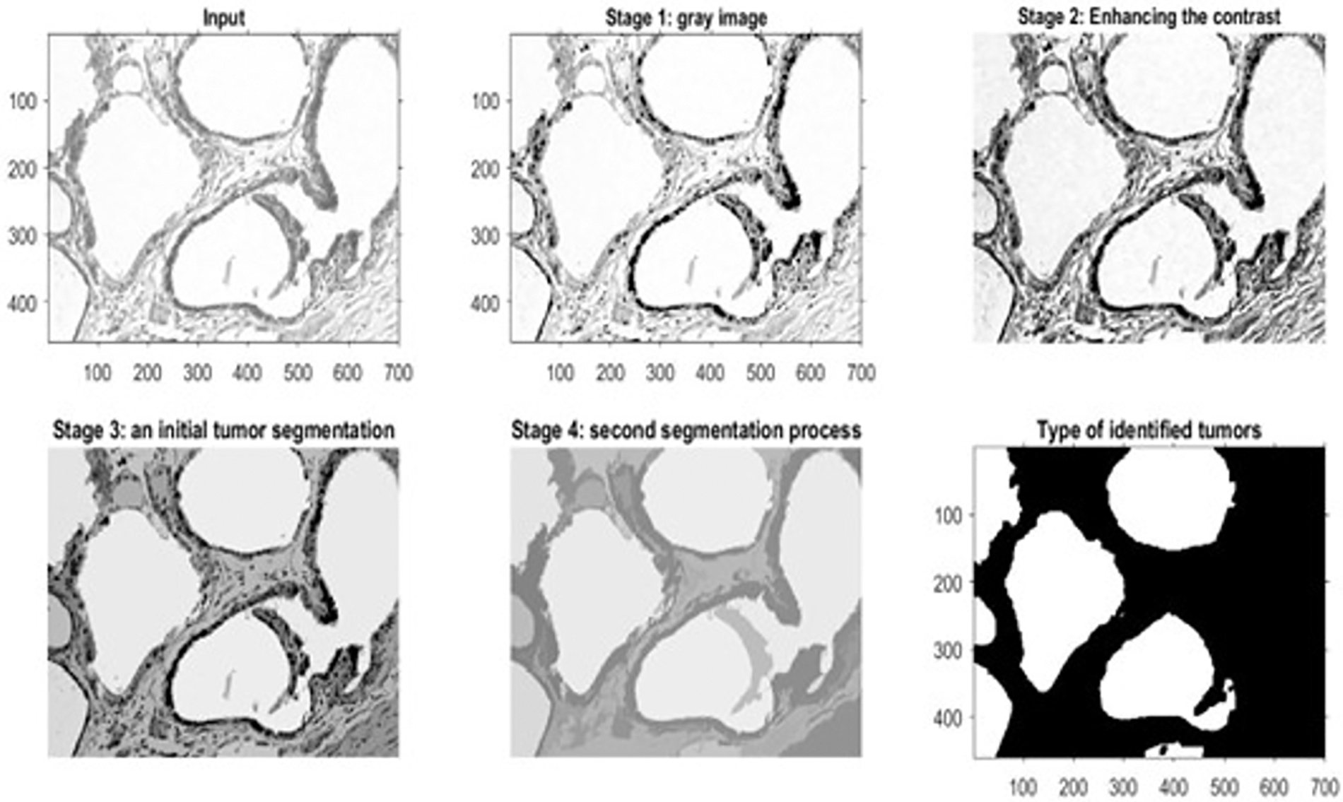
Figure 8: The outputs of a benign histopathology sample

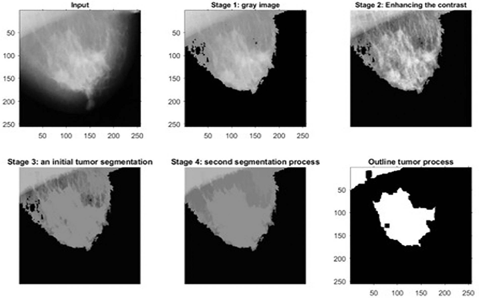
Figure 9: The outputs of a malignant mammographic sample

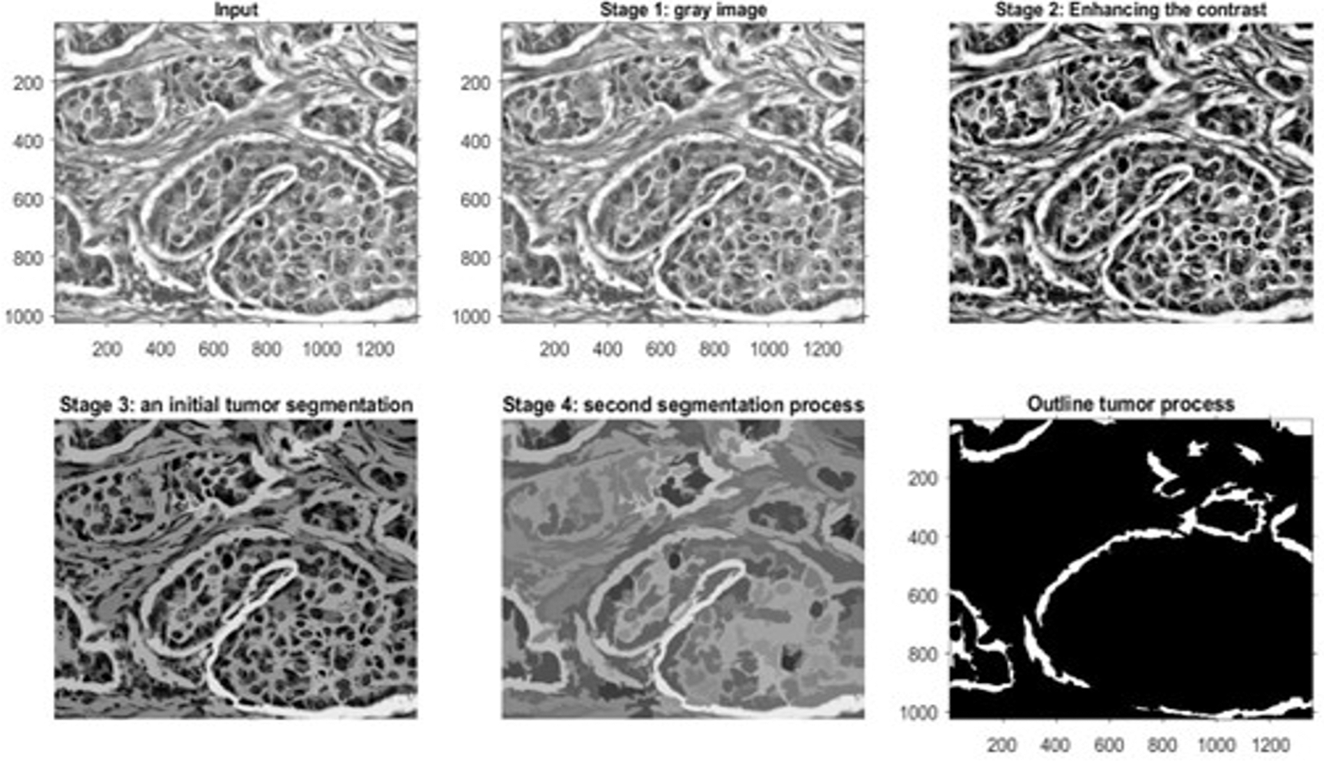
Figure 10: The outputs of a microscopic biopsy malignant sample

Fig. 8 shows the outcomes of the first dataset, which contains histopathological images. These outcomes denote the detected type of breast cancer. Fig. 9 illustrates the results of one sample from the third dataset, a mammographic image, while Fig. 10 represents the results of an example from the fifth dataset. This dataset contains microscopic biopsy images. Every figure includes six subgraphs. These subgraphs present an input sample, a resultant gray image, a contrast enhancement, an initial segmentation stage, a second segmentation stage, and the outlined identified tumor(s). These outputs signify that the presented algorithm properly discovers this disease and classifies its type. Table 8 provides data about the complexity of the presented model in terms of the average processing time per image, floating-Point Operations Per Second (FLOPS), and the total number of utilized parameters in the proposed algorithm.

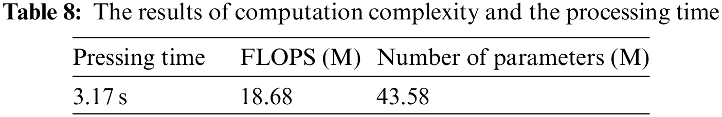
Fig. 11 shows the obtained Receiver Operating Characteristic (ROC) curve by the presented algorithm.

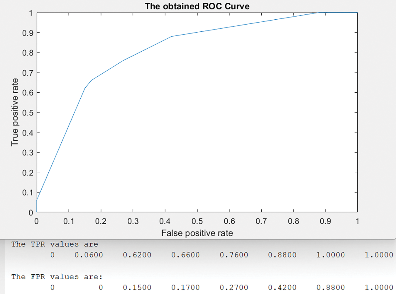
Figure 11: The achieved ROC curve

In the ROC curve, eight threshold values between [0, 1] were used as shown in Fig. 11. For each threshold value, the system calculated the corresponding results of True Positive Ratio (TPR) and False Positive Ratio (FPR) as displayed in the same figure. The best validation of Mean Squared Error (MSE) occurs at epoch 12 with a value = 0.00024845. The evaluated results of the presented algorithm indicate that it distinguishes and categorizes breast tumors, small or big, with higher accuracy than developed methods. Table 4 shows all values of the presented model when it is applied to a test dataset with two K-Fold Cross-Validation techniques and K = 5 and 10. Fig. 6 depicts the results of all considered performance parameters between two modules: Scenario 1 and Scenario 2. Table 5 provides insight into how many data inputs were distinguished and correctly classified. Fig. 6 demonstrates the proposed method’s graphical representation of the obtained classification results, while Table 6 depicts the achieved confusion matrix. The correctly detected and classified tumors are highlighted in green, while the improperly identified and categorized tumors are shown in red. Table 7 displays the comparative evaluation analysis and results between some developed models and the presented method. These findings show that the proposed model surpasses all other algorithms on all considered metrics. No previously presented technique reaches the accuracy rate obtained by the implemented approach in this study. Fig. 7 similarly demonstrates accuracy, F-score analysis, and comparison between the proposed method’s developed models in [1,2,8,12]. Both analyses show that the presented algorithm yields the best results of any extant technology for breast cancer detection and classification.

The proposed method in this study customizes and integrates two (DCNNs), AlexNet and ResNet50, to achieve the highest outcomes. These two tools are incorporated with the KNN algorithm to perform intensive learning, detection, and classification operations. The findings show that the resulting method perfectly identifies and categorizes tumors, as depicted in the preceding diagrams. The processing time of the 10-Fold Cross-Validation when L2 = 0.0001 was 21 min when the proposed method ran for 2542 iterations, which indicates that the method operates at an adequately rapid rate. Even with the quick processing time, this model achieves 99.7% accuracy with a 99.85% F-score, providing exquisite findings and confirming that the method is applicable and can be employed in healthcare facilities effectively and immediately.

The current challenges that physicians and pathologists face are how to detect breast cancer early, how to perform the identification at a low cost, and last, but not least, how to reduce death rates by providing treatment as soon as possible. These challenges are best addressed with a practical, reliable, and trustworthy system that requires no special hardware and operates cost-effectively.

5  Conclusion

The approach presented in this study shows a robust, accurate, beneficial, and economical model to appropriately distinguish and accurately categorize breast cancers from different modalities, mammographic, MRI, and histopathological images. This method involves various filters and tools, such as the Gabor filter, DWT, PCA, KNN, ResNet50, and AlexNet, to produce favorable conclusions. The implemented model has the very critical ability to classify cancers as malignant or benign, allowing physicians to address any cancer as its seriousness requires. Normal, healthy tissue, referred to as healthy in this research, are also able to be categorized. The proposed algorithm was evaluated and tested on the five datasets. The obtained outcomes mark that the implemented model outstands all other implemented models regarding all considered quantities. The accuracy is enhanced by 0.598% compared to what was achieved. Finally, the implemented model delivers considerable enhancements regarding accuracy and F-score. Moreover, the execution time for this approach improves quietly and more quickly than preexisting models. The limitation of the presented model is in the specificity parameter, and its estimation is less than other considered quantities.

In future work, the authors hope to develop a novel model to detect breast tumors using blood or urine samples. We hope every future model made can predict the disease quickly with less than 5% of an acceptable error margin.

Acknowledgement: The authors extend their appreciation to the Deanship of Scientific Research at Northern Border University, Arar, KSA for funding this research work through the project number “NBU-FFR-2023-0009”.

Funding Statement: The authors extend their appreciation to the Deanship of Scientific Research at Northern Border University, Arar, KSA for funding this research work through the project number “NBU-FFR-2023-0009”.

Conflicts of Interest: The authors declare that they have no conflicts of interest to report regarding the present study.

References

1. A. Alsheikhy, Y. Said, T. Shawly, A. K. Alzahrani and H. Lahza, “Biomedical diagnosis of breast cancer using deep learning and multiple classifiers,” Diagnostics, vol. 12, no. 11, pp. 1–15, 2022. [Google Scholar]

2. E. Akkur, F. Turk and O. Erogul, “Breast cancer diagnosis using feature selection approaches and Bayesian optimization,” Computer Systems Sciences and Engineering, vol. 45, no. 2, pp. 1017–1031, 2023. [Google Scholar]

3. M. J. Umer, M. Sharif, M. Alhaisoni, U. Tariq, Y. J. Kim et al., “A framework of deep learning and selection-based breast cancer detection from histopathology images,” Computer Systems Sciences and Engineering, vol. 45, no. 2, pp. 1001–1016, 2023. [Google Scholar]

4. M. Drinkovic, I. Drinkovic, D. Milevcic, F. Matijevic, V. Drinkovic et al., “Diagnostic and practical value of abbreviated contrast enhanced magnetic resonance imaging in breast cancer diagnostics,” Cancers, vol. 14, no. 22, pp. 1–13, 2022. [Google Scholar]

5. W. Ming, F. Li, Y. Zhu, Y. Bai, W. Gu et al., “Unsupervised analysis based on DCE-MRI radiomics features revealed three novel breast cancer subtypes with distinct clinical outcomes and biological characteristics,” Cancers, vol. 14, no. 22, pp. 1–20, 2022. [Google Scholar]

6. R. Benaka, D. Szaboova, Z. Gulasova, Z. Hertelyova and J. Radonak, “Classic and new markers in diagnostics and classification of breast cancer,” Cancers, vol. 14, no. 22, pp. 1–22, 2022. [Google Scholar]

7. M. Madani, M. M. Behzadi and S. Nabavi, “The role of deep learning in advancing breast cancer detection using different imaging modalities: A systematic review,” Cancers, vol. 14, no. 22, pp. 1–36, 2022. [Google Scholar]

8. C. W. Wang, K. Y. Lin, M. A. Khalil, K. L. Chu and T. K. Chao, “A soft label deep learning to assist breast cancer target therapy and thyroid cancer diagnosis,” Cancers, vol. 14, no. 22, pp. 1–30, 2022. [Google Scholar]

9. T. M. Hanis, N. I. R. Ruhaiyem, W. N. Arifin, J. Haron, W. F. W. Abdul Rahman et al., “Over-the-counter breast cancer classification using machine learning and patient registration record,” Diagnostics, vol. 12, no. 11, pp. 1–19, 2022. [Google Scholar]

10. S. H. Shovon, J. Islam, M. N. A. K. Nabil, M. Molla, A. I. Jony et al., “Strategies for enhancing the multi-stage classification performances of HER2 breast cancer from hematoxylin and eosin images,” Diagnostics, vol. 12, no. 11, pp. 1–21, 2022. [Google Scholar]

11. D. S. Gahrouei, F. Aminolroayaei, H. Nematollahi, M. Ghaderian and S. S. Gahrouei, “Advanced magnetic resonance imaging modalities for breast cancer diagnosis: An overview of recent findings,” Diagnostics, vol. 12, no. 11, pp. 1–18, 2022. [Google Scholar]

12. G. Ayana and S. W. Choe, “BUVITNET: Breast ultrasound detection via vision transformers,” Diagnostics, vol. 12, no. 11, pp. 1–14, 2022. [Google Scholar]

13. J. Jayandhi, J. S. L. Jasmine and S. M. Joans, “Mammogram learning system for breast cancer diagnosis using deep learning SVM,” Computer Systems Sciences and Engineering, vol. 40, no. 2, pp. 491–503, 2022. [Google Scholar]

14. D. S. Cherlin, J. Mwaiselage, K. Msami, Z. Heisler, H. Young et al., “Breast cancer screening in low-income countries: A new program for downstaging breast cancer in Tanzania,” BioMed Research International, vol. 2022, Article ID 9795534, pp. 9, 2022. [Google Scholar]

15. X. Jia, X. Sun and X. Zhang, “Breast cancer identification using machine learning,” Mathematical Problem in Engineering, vol. 2022, Article ID 8122895, pp. 8, 2022. [Google Scholar]

16. M. U. Nasir, T. M. Ghazal, M. A. Khan, M. Zubair, A. Rahman et al., “Breast cancer prediction empowered with fine-tuning,” Computational Intelligence and Neuroscience, vol. 2022, Article ID 5918686, pp. 9, 2022. [Google Scholar]

17. A. Rasool, C. Buntemgchit, L. Tiejian, R. Islam, Q. Qu et al. “Improved machine learning-based predictive models for breast cancer diagnosis,” International Journal of Environmental Research and Public Health, vol. 19, no. 6, pp. 1–19, 2022. [Google Scholar]

18. J. Nebhan and P. M. Ferreira, “A chopper negative-r delta-sigma ADC for audio MEMS sensors,” Computer Modeling in Engineering & Sciences, vol. 130, no. 2, pp. 607–631, 2022. [Google Scholar]

19. G. Bianchini, C. D. Angelis, L. Licata and L. Gianni, “Treatment landscape of triple-negative breast cancer expanded options, evolving needs,” Nature Reviews Clinical Oncology, vol. 19, no. 2, pp. 91–113, 2022. [Google Scholar] [PubMed]

20. N. Harbeck, F. P. Liorca, J. Cortes, M. Gnant, N. Houssami et al., “Breast cancer,” Nature, vol. 5, no. 1, pp. 1–29, 2019. [Google Scholar]

21. E. S. McDonald, A. S. Clark, J. Tchou, P. Zhang and G. M. Freedman, “Clinical diagnosis and management of breast cancer,” The Journal of Nuclear Medicine, vol. 57, no. 2, pp. 9s–16s, 2016. [Google Scholar] [PubMed]

22. B. Smolarz, A. Z. Nowak and H. Romanowicz, “Breast cancer-epidemiology, classification, pathogenesis and treatment (review of literature),” Cancer, vol. 14, no. 10, pp. 1–27, 2022. [Google Scholar]

23. S. Rajagopal, T. Thanarajan, Y. Alotaibi and S. Alghamdi, “Brain tumor: Hybrid feature extraction based on unet and 3dcnn,” Computer Systems Science and Engineering, vol. 45, no. 2, pp. 2093–2109, 2023. [Google Scholar]

24. A. F. Subah, O. I. Khalaf, Y. Alotaibi, R. Natarajan, N. Mahadev et al., “Modified self-adaptive Bayesian algorithm for smart heart disease prediction in IoT system,” Sustainability, vol. 14, no. 21, pp. 14208, 2022. [Google Scholar]

25. M. O. Adebiyi, M. O. Arowolo, M. D. Mshelia and O. O. Olugbara, “A linear discriminant analysis and classification model for breast cancer diagnosis,” Applied Sciences, vol. 12, pp. 11455, 2022. [Google Scholar]

26. M. O. Adebiyi, J. O. Afolayan, M. O. Arowolo, A. K. Tyagi and A. A. Adebiyi, “Breast cancer detection using a PSO-ANN machine learning technique,” In: T. Amit Kumar, (Ed.Using Multimedia Systems, Tools, and Technologies for Smart Healthcare Services, Chapter No. 7, pp. 96–116, New Delhi, India: National Institute of Fashion Technology, IGI Global, 2022. [Google Scholar]

27. J. O. Afolayan, M. O. Adebiyi, M. O. Arowolo, C. Chakraborty and A. A. Adebiyi, “Breast cancer detection using particle swarm optimization and decision tree machine learning technique,” in Intelligent Healthcare Infrastructure, Algorithms and Management, Singapore: Springer, pp. 61–83, 2022. [Google Scholar]

28. Z. Rauf, A. Sohail, S. H. Khan, A. Khan, J. Gwak et al. “Attention-guided multi-scale deep object detection framework for lymphocyte analysis in IHC histology images,” Microscopy, vol. 72, no. 1, pp. 27–42, 2022. [Google Scholar]

29. F. A. Spanhol, L. S. Oliveira, C. Petitjean and L. Heutte, “A dataset for breast cancer histopathological image classification,” IEEE Transaction on Biomedical Engineering, vol. 63, no. 7, pp. 1455–1462, 2016. [Google Scholar]

30. A. S. Alsolami, W. Shalash, W. Alsaggaf, S. Ashoor, H. Refaat et al., “King abdulaziz university breast cancer mammogram dataset (KAU-BCMD),” Data, vol. 6, no. 11, pp. 1–15, 2022. [Google Scholar]

31. A. Aksac, D. J. Demetrick, T. Ozyer and R. Alhajj, “BreCaHAD: A dataset for breast cancer histopathological annotation and diagnosis,” BMC Research Notes, vol. 12, pp. 1–3, 2019. [Google Scholar]

32. J. Lu, Y. Wu, M. Hu, Y. Xiong, Y. Zhou et al. “Breast tumor computer-aided detection system based on magnetic resonance imaging using convolutional neural network,” Computer Modeling in Engineering and Sciences, vol. 130, no. 1, pp. 365–377, 2022. [Google Scholar]

33. M. M. Zafar, Z. Rauf, A. Sohail, A. R. Khan, M. Obaidullah et al. “Detection of tumour infiltrating lymphocytes in CD3 and CD8 stained histopathological images using a two-phase deep CNN,” Photodiagnosis and Photodynamic Therapy, vol. 37, no. 102676, pp. 1–32, 2022. [Google Scholar]