Spatial Correlation Module for Classification of Multi-Label Ocular Diseases Using Color Fundus Images

1  Introduction

Over the last several decades, an alarming increase in the prevalence of vision-threatening OD disorders such as age-related macular degeneration (AMD), diabetic retinopathy (DR), cataracts, and uncorrected refractive errors, as well as trachoma, has been seen. The results of a recent study on the vision that was carried out by the World Health Organization (WHO) indicate that the number of individuals all over the world who suffer from some kind of visual impairment has now surpassed 2.2 billion. At least 45 percent of these potential outcomes were either avoidable or do not currently have a remedy that is considered to be adequate [1]. Blindness and other kinds of visual impairment (such as myopia, astigmatism, hypermetropia, and presbyopia) are most often caused by trachoma, cataracts, and uncorrected refractive issues [2]. The WHO estimates that more than 153 million people have some form of visual impairment as a consequence of uncorrected refractive problems; approximately 18 million people are bilaterally blind as a result of cataracts; and approximately one million people have been identified as having trachoma. Research has shown that AMD, which is responsible for 8.7% of all occurrences of blindness globally, is the leading cause of blindness, especially in industrialized nations (or 3 million people). The number of cases is projected to reach 10 million by the year 2040, according to current projections [3]. In addition, recent research [4–6] has shown that DR is responsible for 4.8% of the 37 million cases of blindness that are reported worldwide (i.e., 1.8 million persons). According to the WHO [6], more than 171 million people throughout the globe were living with diabetes in the year 2000. It is expected that this population would reach 366 million by the year 2030 [7]. A little under half of people who have diabetes are unaware that they have the ailment. About two percent of those who have diabetes will become blind, and the other ten percent will have serious visual impairment after 15 years [8]. In addition, after having diabetes for 20 years, around 75% of patients will have some form of diabetic complication [9]. As a consequence of this, the diagnosis and treatment of ODs as soon as possible are very necessary to forestall the irreversible loss of vision [10]. Because they cause damage to the retina, persistent floaters have the potential to cause a loss of vision that is irreversible, and maybe even total blindness [11–13]. Several different imaging methods have been developed throughout the years as a means of assisting in the detection of ODs. Two imaging methods that are often used are CFI and optical coherence tomography (OCT) [14]. The OCT creates cross-sectional images of the retina, and eye issues may be diagnosed by measuring the thickness of the retina [15]. To identify any possible problems, CFI performs monitoring of the inside surfaces of the eyes. Both of these diagnostic approaches are effective in the early-stage diagnosis of ODs. CFI, on the other hand, is a more cost-effective and efficient method, and frequent fundus examination with CFI is advised for asymptomatic patients, particularly the elderly [16,17]. The advancement of many common types of OD, such as diabetic retinopathy (DR), cataracts, and AMD, begins with very few early visual signs [18]. This makes it difficult to accurately diagnose the disease in its early stages. In addition, human review of the vast amounts of data that are supplied by CFI is a process that is both challenging and time-consuming [19]. There is a scarcity of radiologists in less developed regions who are competent to do manual analysis since this method is no longer economically feasible. Not only is there an urgent need for automated models to reduce the amount of labor that ophthalmologists have to do, but they are also required to improve the diagnostic precision of imaging-based procedures [20].

CNN has made major advancements in the realm of medical imaging over the last several years [21,22]. For the diagnosis of ODs, CNNs have shown exceptional performance in a range of fields, ranging from the categorization of diseases to the identification of objects. To locate the fovea centers in OCT photographs, Liefers et al. [9] used a classification method that worked pixel by pixel. Meng et al. [14] suggested the use of a two-stage CNN model to identify optical discs included inside CFI. Zekavat et al. [15] were able to separate intraretinal fluid from extraretinal fluid on OCT images by using CNNs. To segregate the multiple retinal layers and accumulated fluid in OCT images, Gu et al. [5] built an encoder-decoder network that they called ReLayNet. Retinal vessels were segmented in CFI by Zhang et al. [6] using a combination of CNN and connected random fields. Despite the remarkable results, relatively little research has been done to address the problem of multi-label OD classification using CFI [23]. Because a single patient may have numerous distinct types of OD, this presents a problem. Because there is a larger probability that patients would suffer from more than one OD, it is vital to optimize models that are capable of handling multi-label OD categorization. According to a study [11], the coexistence of myopia is associated with an increase in the number of false-negative predictions made about the classification of glaucoma patients. Even though previous research has produced outstanding results in their respective aims, these findings may not apply to situations that occur in the real world where it is impossible to avoid encountering complicated circumstances.

In addition to the issues that have previously been brought out, there is a dearth of research that identifies OD on the level of the individual patient. The great majority of current research investigates the issue on the level of the picture by comparing and contrasting the CFI that is generated by the left eye and the right eye when they are considered apart from one another. A patient-level diagnosis that incorporates information from bilateral CFI should contribute to a more successful approach, as shown by research [20], which discovered that the bilateral eyes are tightly related in terms of the development of OD. The diagnosis made at the patient level has the potential to serve as a preliminary screening for individuals who are at a high risk of developing the illness. The study [22] is especially relevant in the context of situations in which it is necessary to maintain ongoing, extensive surveillance of high-risk patients. The vast majority of current CNN-based OD classification research employs networks created for natural picture analysis rather than networks with architectural optimization, which leads to a drop in classification accuracy.

In this study, we discuss the challenge of classifying CFI-based patient-level multi-label OD (PLML_OD) data. The spatial correlation network (SCNet) serves as the foundation for the PLML_OD that has been suggested. The CFI from both the left and right eyes are used as inputs for the model that has been presented. The outputs are the associated probability of a patient developing a certain OD. A backbone CNN module, a SCNet module for feature refinement and fusion, and a classification module for the creation of classification outputs are the key components that make up the model that has been suggested. The process of feature extraction, which consists of the left and right CFI, is the responsibility of the backbone CNN module. A public CFI dataset [23] is used to demonstrate that our proposed PLML_OD model provides impressive classification performance. An extensive investigation of the results was carried out for this research. In particular, we investigate the performance boost brought about by an increase in the number of connections between nodes in a network and show that there is a clear connection between model complexity and performance. The major contributions of this study are given below:

1)   In this study, we propose a novel PLML_OD model based on SCNet. The proposed model contains a backbone CNN (i.e., DenseNet-169) for the classification of seven different types of OD. In addition, SCNet is a one-of-a-kind module that was created to successfully combine the features that were gathered from both the left and right CFI. SCNet, because it takes into account the links between the recovered qualities, results in an improvement of those attributes.

2)   On a CFI dataset that is accessible to the public, the classification performance of our proposed model with the meticulously constructed strategy of feature correlation and fusion achieves a much higher level of success than the performance of several baseline methods that use direct feature concatenation.

3)   The ablation experiments demonstrate that our proposed model produces superior results as compared to the state-of-the-art methods.

The remaining parts of this article will be presented in the following order. Section 2 discusses recent works of literature. In Section 3, the proposed PLML_OD model for OD classification that makes use of CFI is presented in depth. The circumstances of the experiments, the results of the experiments, and an analysis of the suggested technique in comparison to other approaches are discussed in Section 4. The fifth section concludes this investigation. Additionally, future directions are suggested in this section.

2  Literature Review

This section explores the many diagnostic approaches that are currently in use for OD. Additionally, we discuss the limitations that currently exist and highlight the key methods and solutions that are provided by the suggested system to overcome the existing shortcomings. Transfer learning was employed by Wang et al. [24] to extract characteristics of the CFI. Afterward, ML-C which was based on issue transformation was used to apply those features. The authors made use of a multi-label dataset that had a total of eight distinct labels. They employed the histogram equalization technique on images taken in both black and white and color. After that, two different categorization schemes were tried out on the two different photo collections. At last, they determined the average sigmoid output probability by averaging the results of the two models. The poor network speed is making it difficult for them to complete their task since the dataset they are using has a big number of odd ODs that are categorized as “other ailments.” In addition to this, their system suffers from the problem of data imbalance since there is insufficient information for some types of illnesses in their database. As a result, specific information on some of the acquired qualities is unclear. Mayya et al. [25] identified eight DR lesions in CFI by making use of a graph convolution network, also known as a GCN. Laser scars, drusen, cup disc ratio, hemorrhages, retinal arteriosclerosis, microaneurysms, and both hard and soft exudates were some of the eight main forms of DR lesions. For feature extraction, they used ResNet-101, and then after that, they used two convolutional layers, each of which had a 3 × 3 kernel, stride 2, and adaptive max pooling. Finally, they used a fully supervised learning method called XGBoost. The improved accuracy of their model as well as the values for the receiver operating characteristic suggested an increased capacity to recognize laser scars, drusen, and hemorrhage lesions. Their approach, on the other hand, was unable to detect microaneurysms, soft or hard exudates, or hard exudates [12]. This is mostly because microaneurysms, which showed extremely little red dots within the capillaries of the retina, were found to be the cause of the condition. Because of this, the model was unable to differentiate between the backdrop of the CFI and the microaneurysms that were present in them. On the other hand, soft and hard exudate lesions frequently followed a large number of other fundus lesions at the same time, which made it difficult for the model to extract the characteristics of all fundus lesions. The ODIR2019 dataset was used by Dipu et al. [26] to identify eight ODs using transfer learning. They contrasted the findings by analyzing the functioning of many different cutting-edge DL networks, such as Resnet-34, EfficientNet, MobileNetV2, and VGG-16. After putting the cutting-edge algorithm through its training on the dataset that was used, the authors subsequently reported their findings. Through the process of computing the accuracy, they evaluated the overall performance of the models. The models were organized as a result of the accuracy being implemented into VGG-16, Resnet-34, MobileNetV2, and EfficientNet. The authors, on the other hand, did not propose a unique paradigm for the identification of ODs. In addition, the computation of ACC by itself was inadequate to evaluate the performance of the model. In a computer-aided design (CAD) system, Choi et al. [27] suggested using random forest transfer learning in conjunction with VGG-19. This was done to improve the system’s overall performance. By analyzing a relatively limited dataset, they were able to distinguish eight distinct types of OD. They concluded that the number of categories that needed to be identified could be whittled down to three while maintaining the same level of precision. However, after increasing the number of categories to 10, they discovered that the level of accuracy dropped by around thirty percent. The authors attempted to employ an ensemble classifier that contained transfer learning, and as a consequence, they saw a little improvement in accuracy of 5.5% as a direct result of their efforts. Despite the enhancement, the authors were unable to obtain a satisfactory level of performance since the data were flawed and had inconsistencies.

Based on our earlier analysis of the most current studies, we can conclude the limits of their ability to recognize multiple ODs. These limitations are: 1) multi-label classes affect the performance of the model, especially if there are inadequately many training data points. 2) Some systems are too cautious and cannot be deployed in the real world because the data sets that they employ are either inconsistent or insufficient. We provide a novel PLML_OD for correctly diagnosing the different ODs produced by various CNN models via the use of CFI to solve the constraints that have been encountered in the past. To increase the size of the training dataset without incurring the risks of overfitting or data imbalance, we use a method known as the borderline synthetic minority oversampling technique (BL-SMOTE). On the other hand, SMOTE helps to improve the overall performance of the product. Following transformation, we employ BL-SMOTE to maintain the integrity of the labels. In addition, we provide a one-of-a-kind PLML_OD to extract features by making use of SCNet so that we can deliver correct results. The method that has been proposed can assess the possibility of each ailment among the seven ODs that are shown in each image. In the end, we evaluated the performance of the system using a total of six different metrics, and we contrasted our findings with those of other systems and models already in existence.

3  Materials and Methods

This section contains the dataset description, proposed methodology, and the detail of performance evaluation metrics.

3.1 Dataset Description and Data Augmentation

The PLML_OD model that we recommend is instantiated with the use of a CFI dataset that is publically available to the public [23]. Ocular Disease Intelligent Recognition (ODIR-2019), which is part of the 2019 University International Competition, supplies the dataset. The dataset contains eight different categorization groups, including the normal control group (N) and seven illness groups (diabetes (DB), glaucoma (GL), cataract (CA), age-related macular degeneration (AMD), hypertension (HT), myopia (MP), and abnormalities (AB)). Both the CFI and other information, such as the patient’s age, are used in the construction of the labels that are applied at the patient level. There are 5000 examples included with the first version of the CFI, and 4,020 of those instances have been commented on and made available to the public. The distribution of 4,020 patient cases among eight different categories is seen in Fig. 1.

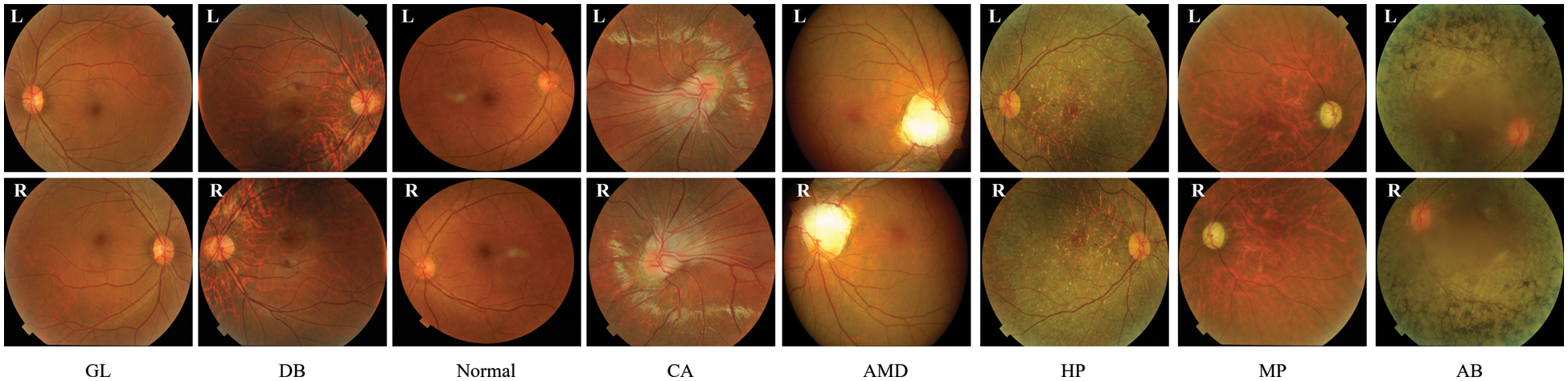
Figure 1: Sample of OD fundus images

We make use of these CFI so that we can assess how well our model operates when it is applied. Training is performed on each combination of the first two folds in the cross-validation process, and testing is performed on the third fold in the process. This is done because the amount of data is not very enormous. Therefore, the BL-SMOTE technique is applied to increase the size of the CFI dataset. The BL-SMOTE method is applied to the minority classes such as GL, CA, AMD, MP, AB, and HT. The detailed summary of the dataset with and without using BL-SMOTE methods is presented in Table 1. The 8,800 cases are split into three folds with a random distribution of 6,160 for training, 880 for validation, and 1,760 for testing respectively. Finally, we provide the average results of the test folds over three different sets of cross-validation tests.

3.2 Proposed Model

The overall layout of the PLML_OD that has been suggested may be seen in Fig. 2. PLML_OD is comprised of its major constituent parts, which are the CNN backbone, the SCNet, and the final classifier.

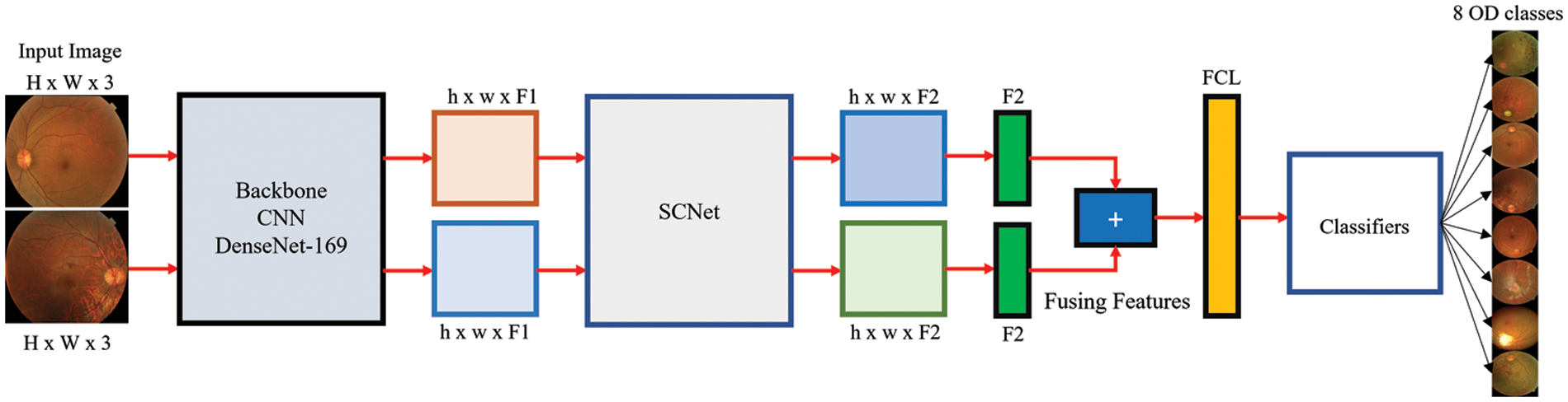
Figure 2: Architecture of proposed PLML_OD model

3.2.1 Backbone CNN

The inputted pairs of CFIs are used to generate two separate sets of features, which are then extracted using CNN. Given the left and right CFI, Ll, and Rr (where Ll, Rr ∈ OH x W x RGB, where the height and width of the input CFIs are denoted by H and W, respectively, and RGB refers to the three-color channels i.e., red, green, and blue), the outputs of the backbone CNN are Dl and Dr (where Dl, Dr ∈ OH x W x F), where F represents the number of extracted features. Since the process of feature extraction does not include the sharing or fusing of any information, there is no need that registration to take place between the paired CFIs. As the backbone of our CNNs, we make use of a wide variety of DenseNet approaches. These approaches do not contain layers that are completely linked to one another.

3.2.2 SCNet

SCNet takes two feature sets from the CNN that acts as its backbone and then constructs two feature sets that correspond to these feature sets by analyzing their correlations. The scheme of SCNet used in this study is shown in Fig. 3.

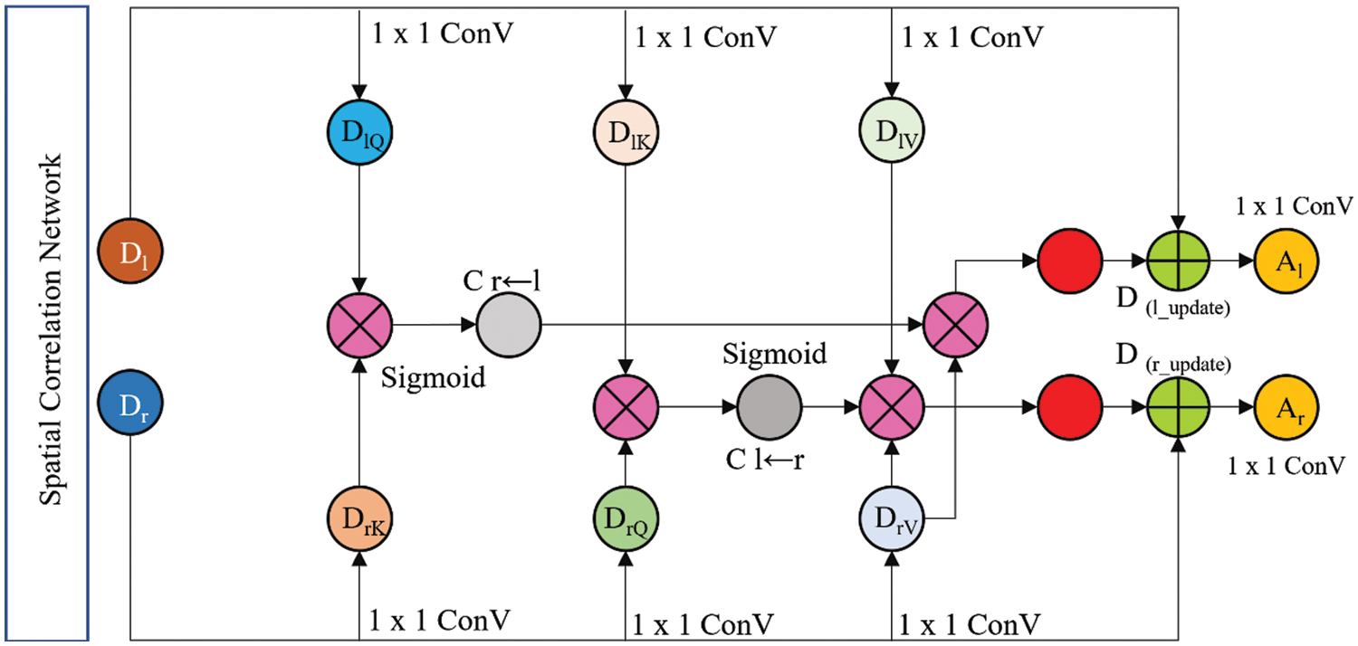
Figure 3: Proposed SCNet architecture

Through the utilization of these sets, it is conceivable to ascertain the pixelwise link that exists between the two input feature sets Ll and Rr. In the beginning, each of the two feature sets is split up into its constituent query (Q), key (K), and value (V) features (DlQ, DlK, and DlV for features of the left CFI, and DrQ, DrK, and DrV for features of the right CFI, where DlQ, DlK, DlV ∈ OH x W x F′, and DrQ, DrK, DrV ∈ OH x W x F′′`) by 1 × 1 convolutions (ConV). Eqs. (1)–(3) are used for extracting features from inputted pairs of CFI.

DIQ=L(Dl;PlQ),DrQ=L(Dr;PrQ)(1)

DlK=L(Dl;PlK),DrK=L(Dr;PrK)(2)

DlV=L(Dl;PlV),DrV=L(Dr;PrV)(3)

where L denotes a linear 1 × 1 ConV and P refers to the pertinent parameters. The dimensions of the converted Q/K and V features are denoted by F′ and F′′, respectively. The empirical value of F′ and F′′ is 1024. The pixel-wise correlation weights were calculated after that by using the transformed features (Cl←r∈O(H×W)(H×W)) are calculated as the inner product adjusted by the sigmoid function (SF). These weights are used to combine the information obtained from the right CFI with that which was retrieved from the left CFI. Eq. (4) is used to aggregate the pairwise correlation by using SF.

Cl←r∈O(H×W)(H×W)=Sigmoid(DlQDrKT)(4)

It is possible to calculate the correlation weights (Cr←l∈O(H×W)(H×W)) like the previous one to combine the information obtained from the left CFI with the information gathered from the right CFI. Eq. (5) is used to measure the correlation weights by using SF.

Cr←l∈O(H×W)(H×W)=Sigmoid(DlQDrKT)(5)

The correlation weights are a representation of the interactions that take place between each CFI site pair. After the weights have been collected, the two sets that were produced from the backbone CNN undergo refinement to their respective values such as Dl_update ∈ OH x W x F′′ and Dr_update ∈ OH x W x F′′ by multiplying the weight maps that correspond to each set. The following Eqs. (6),(7) are used to measure Dl_update and Dr_update:

Dl_update=Cl←r×DrV(6)

Dr_update=Cr←l×DlV(7)

The last element of the SCNet process involves fusing the features that were acquired from the bilateral CFI. Fig. 3 illustrates how the concatenation of four different feature sets leads to the achievement of fusion. In this step, the left input CFI feature set Dl_update is concatenated with the updated left input CFI feature set Dr_update. Eq. (8) is used to measure the SCNet.

M={Al,Ar}(8)

Al=L([Dl,Dl_update]T;PAl)(9)

Ar=L([Dr,Dr_update]T;PAr)(10)

Put Eqs. (9), (10) into Eq. (8). Additionally, Al and Ar are the output of M, and M represents the SCNet (see Eq. (11)).

M={L([Dl,Dl_update]T;PAl),L([Dr,Dr_update]T;PAr)}(11)

3.2.3 Classifiers

To transform the two feature sets that are produced by SCNet into two feature vectors, the process known as global average pooling (GAP) is carried out. After that, they are merged into a single string, and then that string is sent on to the module that does the final classification. The classifier is composed of two fully connected layers (FCLs), of which only one is activated by ReLU and the other is not activated by it. ReLU only triggers one of the FCLs in the classifier. The dimensionality of the concatenated features was lowered as a direct result of the use of the first FCL. This was an immediate consequence of using the first FCL. Consider, for instance, the DenseNet-169 backbone, which is accountable for determining the accurate size of every feature. If one looks at the data that CNN has supplied, one will see that the dimension of the concatenated feature is 2048. After having its value lowered to 1024 by the first FCL, it will remain at that level for the rest of the calculations. When using the second FCL, the features are compressed down to an eighth dimension, which corresponds to the many categories that are used for classification. After this stage has been completed, the eight-dimensional features may be compared to the ground-truth disease classification labels. After this comparison has been made, the network loss can then be determined.

3.2.4 Loss Function

After a softmax activation has been performed, the conventional cross-entropy loss algorithm for eye diseases CFI classification is implemented. This algorithm is more useful in situations where the categories are mutually exclusive. In light of this and taking into account the findings of previous studies [19–21], we use a multi-label soft margin loss to solve the multi-label OD classification issue. The loss function is mathematically expressed in Eq. (12):

L= −1G∑G=1Gr[G]log⁡(σ(O^[G]))+(1−r[G])log(1−σ(O^[G]))(12)

where G denotes the categories, sigmoid activation is denoted by σ, r ∈ {0, 1} the reference label, and the output of the network is represented by O^.

3.3 Performance Metrics

The official ODIR-2019 challenge suggests calculating the kappa score (KS), the F1 score, the area under the receiver operating curve (AUC), accuracy (ACU), and the average (AVG) of the three to evaluate the classification performance of various models. Eqs. (13)–(21) are used to measure these performance metrics. The statistics are computed using the whole dataset, and then they are averaged across all of the patients.

KS=Mo−Me1−Me(13)

Mo=∑h=1hTPh∑h=1h(TPh+FNh)(14)

Me=∑h=1hTPh∗(TPh+FNh)N2(15)

F1score=2TP2TP+FN+FP(16)

AUC=∫a=01TPR(FPR−1(a))dx(17)

TPR=TPTP+FN(18)

FPR=FPFP+TN(19)

ACU=TP+TNTP+TN+FP+FN(20)

AVG=1(KS)+(F1score)+(AUC)(21)

where TP and TN represent the true positive and true negative, respectively. N represents the number of samples used in the process of testing. Additionally, FP shows the value of a false positive, and FN is used to denote the false negative.

4  Results and Discussions

This section shows the experimental findings acquired on the publically available OD dataset, comparing the proposed PLML_OD model to various baselines. Additionally, the ablation study of the proposed model is also performed in this section.

4.1 Experimental Setup

To study the impact that DenseNet models of varying depths have on the process of feature extraction, we use CNNs as the backbone of our system and use DenseNet models. Models that have already been pre-trained on ImageNet are put to use in the process of initializing the backbone CNNs. The CFI has differing resolutions as a result of the fact that the information was acquired from several different sites or hospitals utilizing a variety of devices. First, each CFI is scaled down to a resolution of 299 by 299 pixels. Random cropping of 224 × 224 photo patches is done as part of the image improvement process that is performed during network training. During the testing phase, the alternate method of center cropping is utilized. Keras was used in the implementation of both the proposed PLML_OD model and the baseline models. In addition, the programming of the approaches that are not immediately related to convolutional networks is done in Python. The experiment was carried out using a computer running the Windows operating system, which was equipped with an 11 GB NVIDIA GPU and 32 GB of RAM.

4.2 Models Configuration

The PLML_OD model that has been presented is tuned to perfection by adjusting its many hyperparameters. The stochastic gradient descent (SGD) optimizer is the key tool that is used while training networks with the multi-label classification loss function specified by Eq. (11). The poly learning rate degradation approach is now being used to bring the initial learning rate (LR) down from its setting of 0.001 as a starting point. The intensity level is presently set at 0.90. Each experiment is performed for a total of one hundred epochs, and the information received from the very last epoch is the one that is recorded.

4.3 Results of Classification Using a Variety of Backbones CNNs

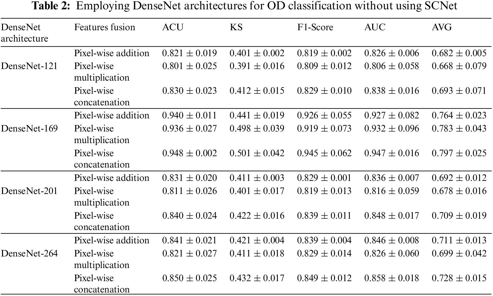
The process of independently obtaining features from bilateral CFI is within CNN's purview. Backbone CNNs with varied depths may extract features with varying degrees of abstraction from the data. Without specifying an explicit fusion technique, the features that are generated by the backbone CNN is instantly combined using addition, pixel-wise multiplication, or concatenation. Table 2 provides a further explanation of the findings. Among the many different processes for fusing, feature concatenation is the one that yields the best results. When working with a CNN that has a deep backbone, pixel-wise multiplication is the method that works best. The second point is that the performance of CNNs with a stronger backbone is superior. When comparing the results of models with a DenseNet-169 backbone and feature concatenation to those with a DenseNet-201, we find that the KS, AUC, F1-score, ACU, and final AVG are all improved by 8.8%, 2.4%, 2.4%, and 4.5%, respectively. It indicates a stronger ability of the OD to differentiate between higher abstraction elements. In conclusion, it has been shown that models that use DenseNet-121 eventually hit a performance plateau, and replacing it with a DenseNet-169 backbone has minimal influence on the situation. Research that is similar to this one reveals that the performance of a network cannot rise linearly with the number of connections between nodes [21]. The three possible explanations for this. The first issue has to do with the problem of the gradient disappearing. When there is more information available, optimizing a network becomes a more difficult task [14]. The second aspect that contributes to the inefficient use of the enormous quantity of features developed for deep networks is a decline in the reuse of those features [15]. Because the network is not fully trained since there are only a limited amount of training samples that may be accessed.

4.4 Improved Classification Performance Using SCNet

The potential results of activating SCNet are outlined in Table 3. Even with an increasing network depth, the general performance trend has not changed, just as was the case before the SCNet was put into place. When dense feature correlations are included in classification models built using SCNet, classification accuracy is increased in a manner that is not reliant on the backbone CNNs and is more constant. Take the model that has a DenseNet-169 for example. The use of SCNet improves the performance of CNN in all four parameters by corresponding percentages of 4.2%, 1.9%, 1.1%, and 1.7%. Comparing the outcomes achieved with and without SCNet with the use of paired t-tests reveals, with a p-value that is less than 0.05, that SCNet may considerably increase classification performance as measured by the KS, the F1-score, and the final AVG score. When alternative backbone CNNs are used, performance reaches a plateau of the same sort as when utilizing the original CNN. The average score of networks that have DenseNet-201 as their backbone is 1.3% higher than the average score of networks that have DenseNet-121 as their backbone. On average, the performance of a network with a DenseNet-169 backbone is 2.4% better than the performance of a network with a DenseNet-121 or DenseNet-201 backbone. However, as compared to networks with DenseNet-201 backbone, those with DenseNet-264 backbone only increase AVG by a meager 0.5%. The comparison of the results obtained using and without using SCNet are graphically presented in Fig. 4. It’s not necessary to use the deepest possible backbone CNN, due to the additional processing complexity that comes along with raising the network depth. This topic will be covered in the part that comes after this one.

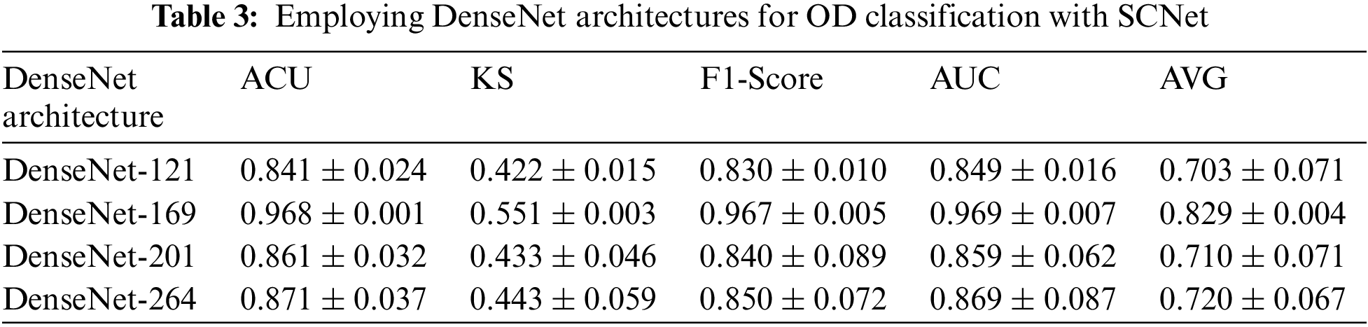
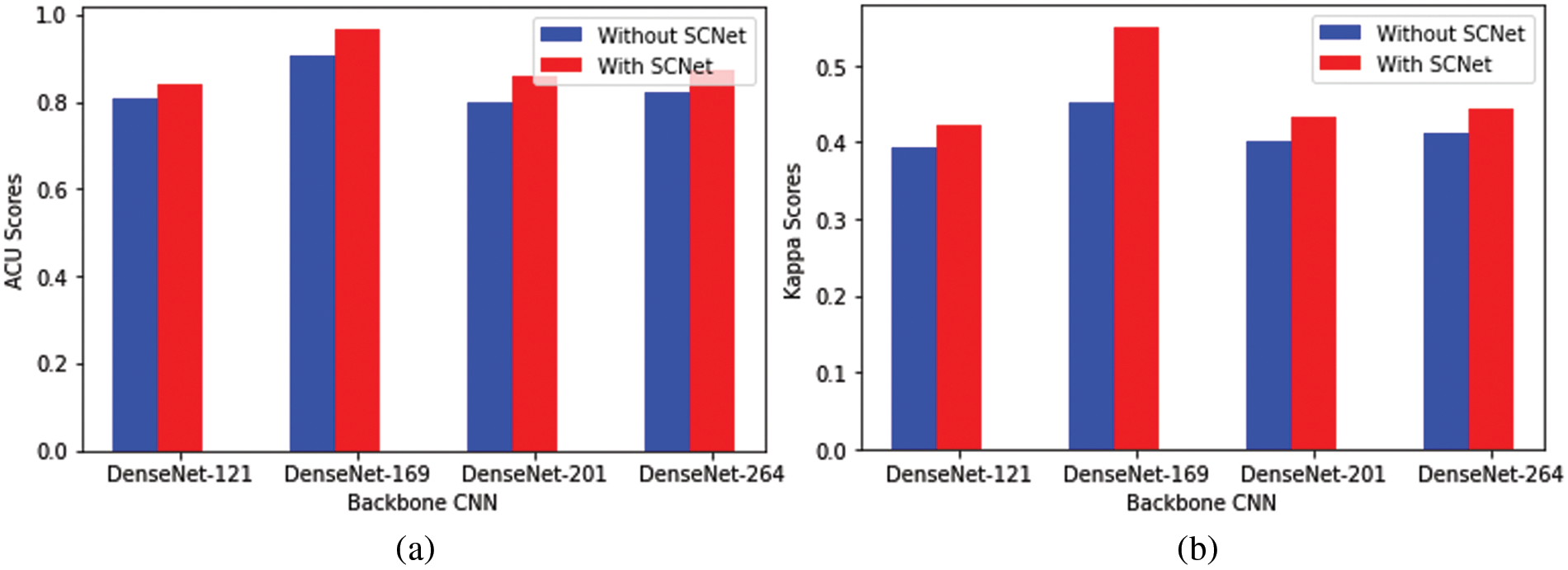
Figure 4: Comparison of the performance of several backbone CNNs for classification. (a) Represents the backbone CNN’s performance with and without using SCNet in terms of ACU, (b) Represents the backbone CNN’s performance with and without using SCNet in terms of Kappa Score

The retrieved features were used to train four backbone CNN classifiers. The grid search approach was used to optimize the hyperparameters. The 5-fold cross-validation method is used to train the models that are being used. To test the model, several different performance criteria were used for the task of detecting different types of OD. Fig. 5 presents the confusion matrices for DenseNet architecture using SCNet. With DenseNet-169, the model identified 215 out of 220 OD instances and incorrectly categorized two cases as CA, one case as DB, one case as HP, and one case as normal. The model correctly predicted the class label for each normal instance. In the example of DenseNet-121 (in which extracted characteristics were utilized to train the model), the model correctly identified 199 cases of AB disease out of 220 total cases but incorrectly labeled 21 cases as normal and other OD diseases such as AMD, CA, DB, GL, HP, and MP. There were 202 instances of AMD illness, and DenseNet-264 correctly predicted their class label. However, 18 cases were incorrectly categorized as normal or other forms of OD. DenseNet-201 correctly predicted the class label for 199 out of 201 DB illness cases. However, it incorrectly identified two instances as normal.

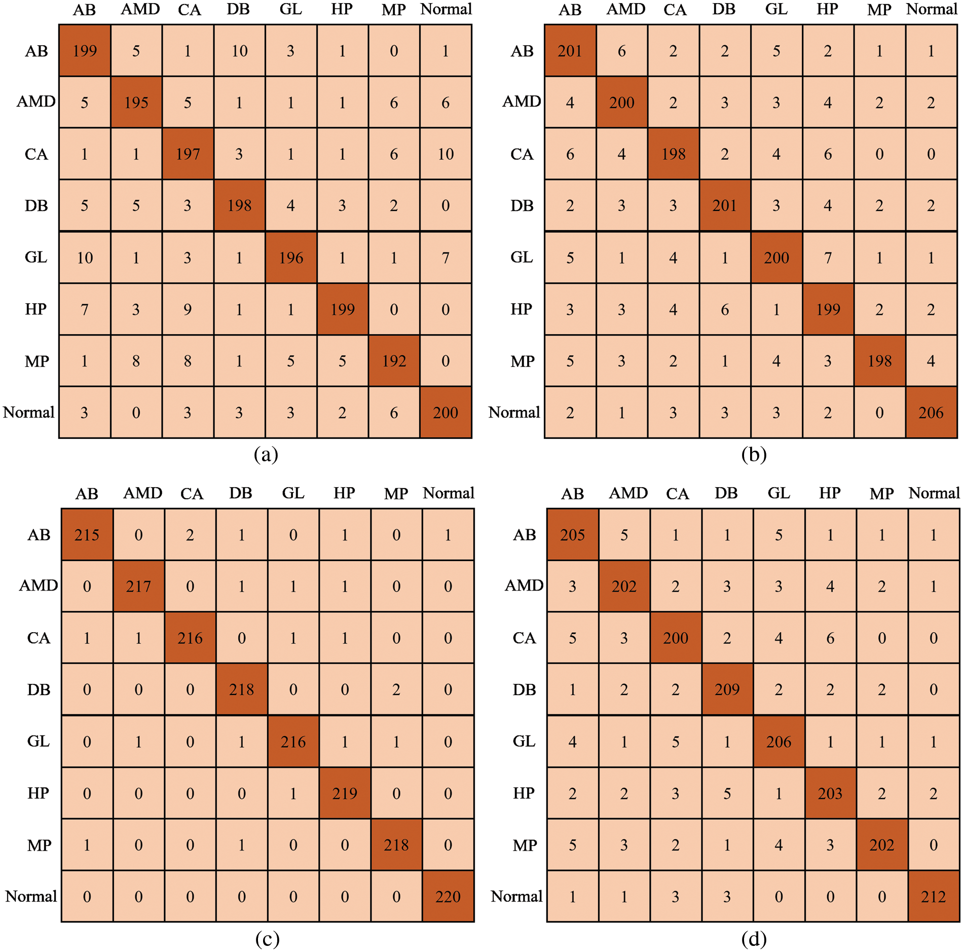
Figure 5: Confusion matrix; (a) DenseNet-121, (b) DenseNet-201, (c) Proposed Model, and (d) DenseNet-264

4.5 DenseNet Architecture Computational Complexities

Table 4 has a description of the complexity of the network, and Fig. 6 contains a presentation of the classification metrics about the number of floating-point operations per second (FLOPs), as well as the parameters of the network. Because of this, we can compare the outcomes of categorization in a way that is both objective and equitable.

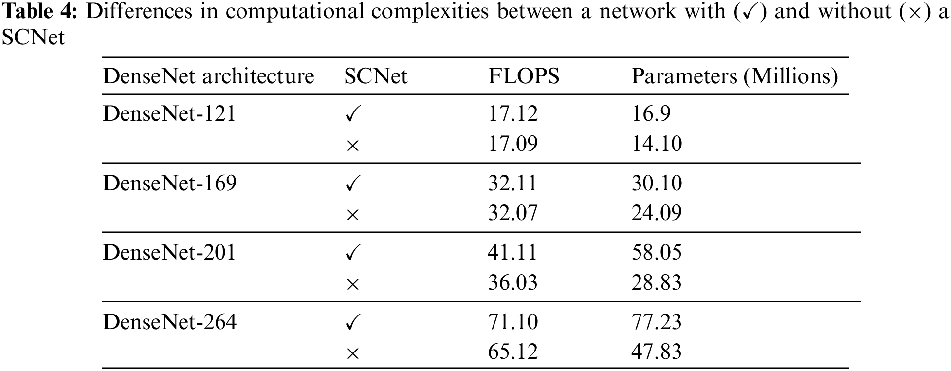
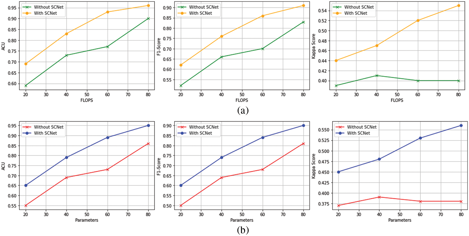
Figure 6: The outcomes of the PLML_OD model that has been proposed (a) Classification performance for FLOPs (b) Configurations for model total trainable parameters

Even when FLOPs or networks are taken into contemplation, the suggested PLML_OD approach may still be much more advanced than the baseline. Networks with a DenseNet-169 backbone and SCNet can outperform baselines with a DenseNet-201 and DenseNet-264 backbone while using a much lower number of FLOPs. This demonstrates that the increasing complexity of networks is not the sole factor contributing to the extremely accurate categorization conclusions produced by the suggested method. It is possible to enhance the categorization of OD at the level of the individual patient by considering the connection between the left and right CFI. To get improved classification performance, it is very necessary to make advantage of the information that is provided by both CFI. This is because the diagnosis at the level of the patient is of great significance [25]. Even if the introduction of SCNet only results in a moderate rise in FLOPs, the network parameters will almost certainly see a significant expansion. This is notably the case for baselines that are supported by the DenseNet-201 and DenseNet-264 backbones.

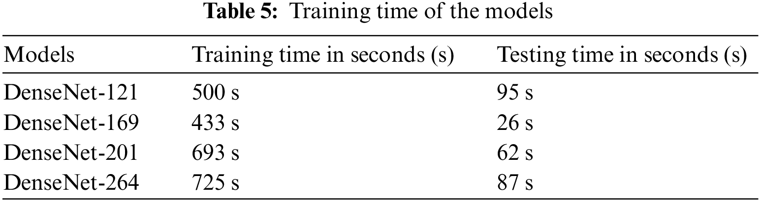
Table 5 presents the training time of the proposed model and other backbone models. The results show that DenseNet-121 takes 500 seconds (s) to train on the entire dataset. The DenseNet-169 and DenseNet-201 models take 433 and 693 s, respectively, to train. The DenseNet-169 model takes less training time as compared to other models. The reason behind this is the total trainable parameters of DenseNet-169 are less than other models (see Fig. 6b).

4.6 Ablation Study

In this research, we worked to design the novel model by including the SCNet, in addition to developing more advanced versions of the DenseNet-169 and the multi-label soft margin loss function. We used the control variable strategy to statistically analyze the experimental data while simultaneously controlling a variable to determine whether or not the proposed PLML_OD model is valid for use with eight OD, including the normal condition. At the time of experiments, the accuracy and kappa score values of each model were investigated and compared with the assistance of metrics to establish the significance of the enhanced module to the model. Experiment 1 demonstrates the basic SCNet model, Experiment 2 demonstrates the implementation of the DenseNet-169 model, and Experiment 3 compares the DenseNet-169 model with a multi-label soft margin loss function and SCNet. Table 6 presents the detailed results of the experiment.

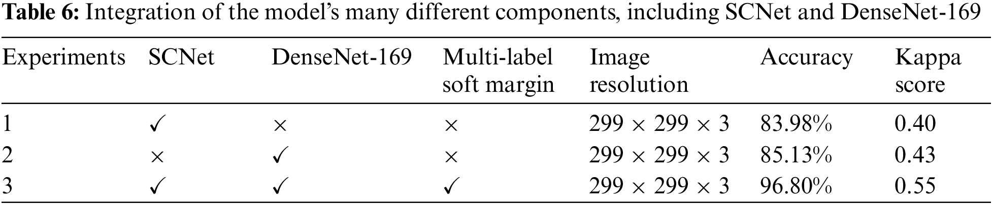
When the results of Experiment 1 are compared with Experiment 2, it is clear that DensNet-169 leads to an improvement of 1.15% in the model’s average OD classification accuracy. When we combined the SCNet and DenseNet with multi-label soft margin loss function to develop the proposed PLML_OD model in Experiment 3. The results reveal that the proposed model improved by 11.67% as compared to Experiment 2 in classifying OD.

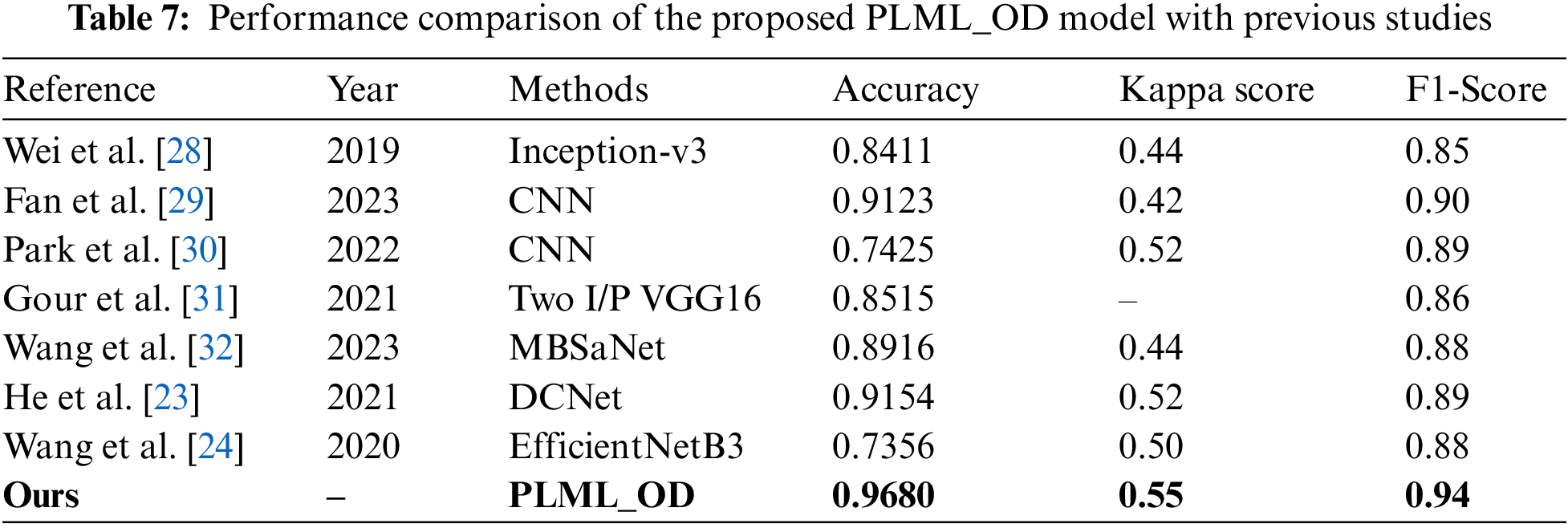
4.7 Comparison with State-of-the-arts

In this subsection, the superior performance of the proposed PLML_OD model is verified by comparing it with state-of-the-art methods. Wei et al. [28] designed a novel inception-v3 model and achieved an accuracy of 0.84 for classifying the ocular disease. In a study [29–31], they developed a CNN model for the detection of glaucoma using a fundus image. They attained an accuracy of 0.91, a Kappa score of 0.42, and an F1 score of 0.90. Wang et al. [32] proposed a novel model named MBSaNet and achieved an accuracy of 0.89. A detailed comparison of the proposed model with previous studies in terms of many evaluation metrics is discussed in Table 7.

5  Conclusion

A classification model for PLML_OD eye illnesses was constructed with the aid of three fundamental modules for this research investigation. These modules included a CNN backbone, a SCNet, and a classifier for the creation of classification scores. The most cutting-edge component of our network's architecture is called SCNet, and it enables pixel-wise feature correlation to be carried out by making use of the two sets of data acquired by the backbone CNN from both the left and the right CFI. After this stage, the processed features are merged to provide a patient-level representation of the features to be ready for the final patient-level OD classification. The classification performance of the proposed model has been evaluated on the publically available dataset of seven different OD. The proposed model achieved a classification accuracy of 96.80% in classifying OD. The result reveals that the proposed model performs superior as compared to the baseline models as well as the state-of-the-art classifiers. We believe that our model would assist the eye specialist in identifying OD. The limitation of the study is that a dataset contains a less number of images and is imbalanced; however, to handle this issue BL-SMOTE is applied. In the future, we will develop a federated learning-based collaborative model with the help of several hospitals by keeping in mind patient data privacy.

Funding Statement: The authors received no specific funding for this study.

Conflicts of Interest: The authors declare that they have no conflicts of interest to report regarding the present study.

References

1. C. Perdomo, J. Oscar and A. G. Fabio, “A systematic review of deep learning methods applied to ocular images,” Ciencia e Ingeniería Neogranadina, vol. 30, no. 1, pp. 9–26, 2022. [Google Scholar]

2. W. Xiao, H. Xi, H. W. Jing, R. L. Duo, Z. Yi et al., “Screening and identifying hepatobiliary diseases through deep learning using ocular images: A prospective, multicentre study,” The Lancet Digital Health, vol. 3, no. 2, pp. e88–e97, 2021. [Google Scholar] [PubMed]

3. Z. Wang, Z. Yuanfu, Y. Mudi, M. Yan, Z. Wenping et al., “Automated segmentation of macular edema for the diagnosis of ocular disease using deep learning method,” Scientific Reports, vol. 11, no. 1, pp. 1–12, 2021. [Google Scholar]

4. P. S. Grewal, O. Faraz, R. Uriel and T. S. T. Matthew, “Deep learning in ophthalmology: A review,” Canadian Journal of Ophthalmology, vol. 53, no. 4, pp. 309–313, 2018. [Google Scholar] [PubMed]

5. H. Gu, G. Youwen, G. Lei, W. Anji, X. Shirong et al., “Deep learning for identifying corneal diseases from ocular surface slit-lamp photographs,” Scientific Reports, vol. 10, no. 1, pp. 1–11, 2020. [Google Scholar]

6. K. Zhang, L. Xiyang, L. Fan, H. Lin, Z. Lei et al., “An interpretable and expandable deep learning diagnostic system for multiple ocular diseases: qualitative study,” Journal of Medical Internet Research, vol. 20, no. 11, pp. e11144, 2018. [Google Scholar] [PubMed]

7. H. Malik, S. F. Muhammad, K. Adel, A. Adnan, N. Q. Junaid et al., “A comparison of transfer learning performance versus health experts in disease diagnosis from medical imaging,” IEEE Access, vol. 8, no. 1, pp. 139367–139386, 2020. [Google Scholar]

8. D. Wang and W. Liejun, “On OCT image classification via deep learning,” IEEE Photonics Journal, vol. 11, no. 5, pp. 1–14, 2019. [Google Scholar]

9. B. Liefers, G. V. Freerk, S. Vivian, V. G. Bram, H. Carel et al., “Automatic detection of the foveal center in optical coherence tomography,” Biomedical Optics Express, vol. 8, no. 11, pp. 5160–5178, 2017. [Google Scholar] [PubMed]

10. T. Nazir, I. Aun, J. Ali, M. Hafiz, H. Dildar et al., “Retinal image analysis for diabetes-based eye disease detection using deep learning,” Applied Sciences, vol. 10, no. 18, pp. 6185, 2020. [Google Scholar]

11. D. S. Q. Ting, R. P. Louis, P. Lily, P. C. John, Y. L. Aaron et al., “Artificial intelligence and deep learning in ophthalmology,” British Journal of Ophthalmology, vol. 103, no. 2, pp. 167–175, 2019. [Google Scholar] [PubMed]

12. O. Ouda, A. M. Eman, A. A. E. Abd and E. Mohammed, “Multiple ocular disease diagnosis using fundus images based on multi-label deep learning classification,” Electronics, vol. 11, no. 13, pp. 1966, 2022. [Google Scholar]

13. T. K. Yoo, Y. C. Joon, K. K. Hong, H. R. Ik and K. K. Jin, “Adopting low-shot deep learning for the detection of conjunctival melanoma using ocular surface images,” Computer Methods and Programs in Biomedicine, vol. 205, pp. 106086, 2021. [Google Scholar] [PubMed]

14. X. Meng, X. Xiaoming, Y. Lu, Z. Guang, Y. Yilong et al., “Fast and effective optic disk localization based on convolutional neural network,” Neurocomputing, vol. 312, no. 2, pp. 285–295, 2018. [Google Scholar]

15. S. M. Zekavat, K. R. Vineet, T. Mark, Y. Yixuan, K. Satoshi et al., “Deep learning of the retina enables phenome-and genome-wide analyses of the microvasculature,” Circulation, vol. 145, no. 2, pp. 134–150, 2022. [Google Scholar] [PubMed]

16. B. Hassan, Q. Shiyin, H. Taimur, A. Ramsha and W. Naoufel, “Joint segmentation and quantification of chorioretinal biomarkers in optical coherence tomography scans: A deep learning approach,” IEEE Transactions on Instrumentation and Measurement, vol. 70, pp. 1–17, 2021. [Google Scholar]

17. Y. Yang, L. Ruiyang, L. Duoru, Z. Xiayin, L. Wangting et al., “Automatic identification of myopia based on ocular appearance images using deep learning,” Annals of Translational Medicine, vol. 8, no. 11, pp. 7–22, 2020. [Google Scholar]

18. K. Y. Wu, K. Merve, T. Cristina, J. Belinda, H. N. Bich et al., “An overview of the dry eye disease in sjögren’s syndrome using our current molecular understanding,” International Journal of Molecular Sciences, vol. 24, no. 2, pp. 1580, 2023. [Google Scholar] [PubMed]

19. L. Faes, K. W. Siegfried, J. F. Dun, L. Xiaoxuan, K. Edward et al., “Automated deep learning design for medical image classification by health-care professionals with no coding experience: A feasibility study,” The Lancet Digital Health, vol. 1, no. 5, pp. 232–242, 2019. [Google Scholar]

20. J. Kanno, S. Takuhei, I. Hirokazu, I. Hisashi, Y. Yuji et al., “Deep learning with a dataset created using kanno saitama macro, a self-made automatic foveal avascular zone extraction program,” Journal of Clinical Medicine, vol. 12, no. 1, pp. 183, 2023. [Google Scholar]

21. P. Li, L. Lingling, G. Zhanheng and W. Xin, “AMD-Net: Automatic subretinal fluid and hemorrhage segmentation for wet age-related macular degeneration in ocular fundus images,” Biomedical Signal Processing and Control, vol. 80, no. 2, pp. 104262, 2023. [Google Scholar]

22. C. S. Lee, J. T. Ariel, P. D. Nicolaas, W. Yue, R. Ariel et al., “Deep-learning based, automated segmentation of macular edema in optical coherence tomography,” Biomedical Optics Express, vol. 8, no. 7, pp. 3440–3448, 2017. [Google Scholar] [PubMed]

23. J. He, L. Cheng, Y. Jin, O. Yu and G. Lixu, “Multi-label ocular disease classification with a dense correlation deep neural network,” Biomedical Signal Processing and Control, vol. 63, no. 24, pp. 102167, 2021. [Google Scholar]

24. J. Wang, Y. Liu, H. Zhanqiang, H. Weifeng and L. Junwei, “Multi-label classification of fundus images with efficientnet,” IEEE Access, vol. 8, pp. 212499–212508, 2020. [Google Scholar]

25. V. Mayya, K. Uma, K. S. Divyalakshmi and U. A. Rajendra, “An empirical study of preprocessing techniques with convolutional neural networks for accurate detection of chronic ocular diseases using fundus images,” Applied Intelligence, vol. 53, no. 2, pp. 1548–1566, 2023. [Google Scholar] [PubMed]

26. N. M. Dipu, A. S. Sifatul and K. Salam, “Ocular disease detection using advanced neural network based classification algorithms,” Asian Journal for Convergence In Technology, vol. 7, no. 2, pp. 91–99, 2021. [Google Scholar]

27. J. Y. Choi, K. Y. Tae, G. S. Jeong, K. Jiyong, T. U. Terry et al., “Multi-categorical deep learning neural network to classify retinal images: A pilot study employing small database,” PloS One, vol. 12, no. 11, pp. e0187336, 2017. [Google Scholar] [PubMed]

28. D. Wei, P. Ning, L. Si-Yu, W. Yan-Ge and T. Ye, “Application of iontophoresis in ophthalmic practice: An innovative strategy to deliver drugs into the eye,” Drug Delivery, vol. 30, no. 1, pp. 2165736, 2023. [Google Scholar] [PubMed]

29. R. Fan, A. Kamran, B. Christopher, C. Mark, B. Nicole et al., “Detecting glaucoma from fundus photographs using deep learning without convolutions: Transformer for improved generalization,” Ophthalmology Science, vol. 3, no. 1, pp. 100233, 2023. [Google Scholar] [PubMed]

30. K. B. Park and Y. L. Jae, “SwinE-Net: Hybrid deep learning approach to novel polyp segmentation using convolutional neural network and Swin Transformer,” Journal of Computational Design and Engineering, vol. 9, no. 2, pp. 616–632, 2022. [Google Scholar]

31. N. Gour and K. Pritee, “Multi-class multi-label ophthalmological disease detection using transfer learning based convolutional neural network,” Biomedical Signal Processing and Control, vol. 66, no. 3, pp. 102329, 2021. [Google Scholar]

32. K. Wang, X. Chuanyun, L. Gang, Z. Yang, Z. Yu et al., “Combining convolutional neural networks and self-attention for fundus diseases identification,” Scientific Reports, vol. 13, no. 1, pp. 1–15, 2023. [Google Scholar]