
 Submit a Paper
 Propose a Special lssue
 Open Access
ARTICLE
Increasing Crop Quality and Yield with a Machine Learning-Based Crop Monitoring System
1 College of Information Science Technology, Hainan Normal University, Haikou, 571158, China
2 School of Information Engineering, Qujing Normal University, Qujing, 655011, China
3 Department of Computer Science, COMSATS University, Islamabad, 45550, Pakistan
* Corresponding Authors: Anas Bilal. Email: ; Haixia Long. Email:
Computers, Materials & Continua 2023, 76(2), 2401-2426. https://doi.org/10.32604/cmc.2023.037857
Received 18 November 2022; Accepted 19 June 2023; Issue published 30 August 2023
 View Full Text
 Download PDF
Abstract
Farming is cultivating the soil, producing crops, and keeping livestock. The agricultural sector plays a crucial role in a country’s economic growth. This research proposes a two-stage machine learning framework for agriculture to improve efficiency and increase crop yield. In the first stage, machine learning algorithms generate data for extensive and far-flung agricultural areas and forecast crops. The recommended crops are based on various factors such as weather conditions, soil analysis, and the amount of fertilizers and pesticides required. In the second stage, a transfer learning-based model for plant seedlings, pests, and plant leaf disease datasets is used to detect weeds, pesticides, and diseases in the crop. The proposed model achieved an average accuracy of 95%, 97%, and 98% in plant seedlings, pests, and plant leaf disease detection, respectively. The system can help farmers pinpoint the precise measures required at the right time to increase yields.Keywords
Nomenclature
| AI | Artificial Intelligence |
| ML | Machine learning |
| DL | Deep learning |
| IoT | Internet of Things |
| SVM | Support vector machine |
| CNN | Convolutional neural networks |
| RBF | Radial basis function |
| SVD | Singular value decomposition |
| IV3 | Iveption-V3 |
Most people think of ‘agriculture’ as cultivating crops and rearing livestock. It makes a significant contribution to a nation’s overall economic health. Agriculture is responsible for producing plenty of raw materials and processed food items. Textile and other industrial sectors rely on cotton and jute, among other natural resources, to create a wide range of goods. Providing food and raw materials for other industries is a significant benefit of agriculture. Crops were grown using time-honored methods passed down from generation. Most individuals throughout the globe frame their documents using traditional methods. It includes farming practices that farmers have recommended with more expertise. Even in the modern age of computing, a country’s progress is tied to its ability to produce crops and be self-sufficient in agricultural products [1]. The quantity of food available depends on the quality of agriculture. Still, with the world’s population expanding at an alarming rate, farmers have had to abandon vast swaths of land, and the resulting decline in soil fertility is plain to see [2]. Due to the imprecision of these methods, a significant amount of effort and time will need to be invested. Smart farming is closely linked to digital technology, including robots, electronic gadgets, sensors, and automation tools.
Smart agriculture has replaced conventional farming due to the smart agriculture road plan in the agricultural business. Humans have been cultivating the earth to get food for sustenance. Agriculture is a technique that has long evolved from version 1.0 to version 4.0. Farmers utilized agricultural implements, including a sickle and a pitchfork, throughout the seventeenth century, known as Agriculture 1.0 [3]. The roadmap of agricultural generations from 1.0 to 4.0, shown in Fig. 1, aids researchers in understanding the many problems and challenges encountered in smart farming. People and animals carried out the tasks during the first agricultural revolution when agriculture operations were organized customarily. The second agricultural revolution brought about some changes, but the bulk of the labor was still manual and time-consuming. The third generation saw the introduction of new technology that made the growth of agricultural operations more practical. But inadequate knowledge and a lack of expertise result in poor management of the farming activity. The era of modern agriculture has changed since the fourth generation with its array of technologies, including big data, blockchain, machine learning, swarm intelligence, cyber-physical systems, deep learning, Internet of Things (IoT), autonomous robotics systems, generative adversarial networks, and cloud edge-fog computing emerged.
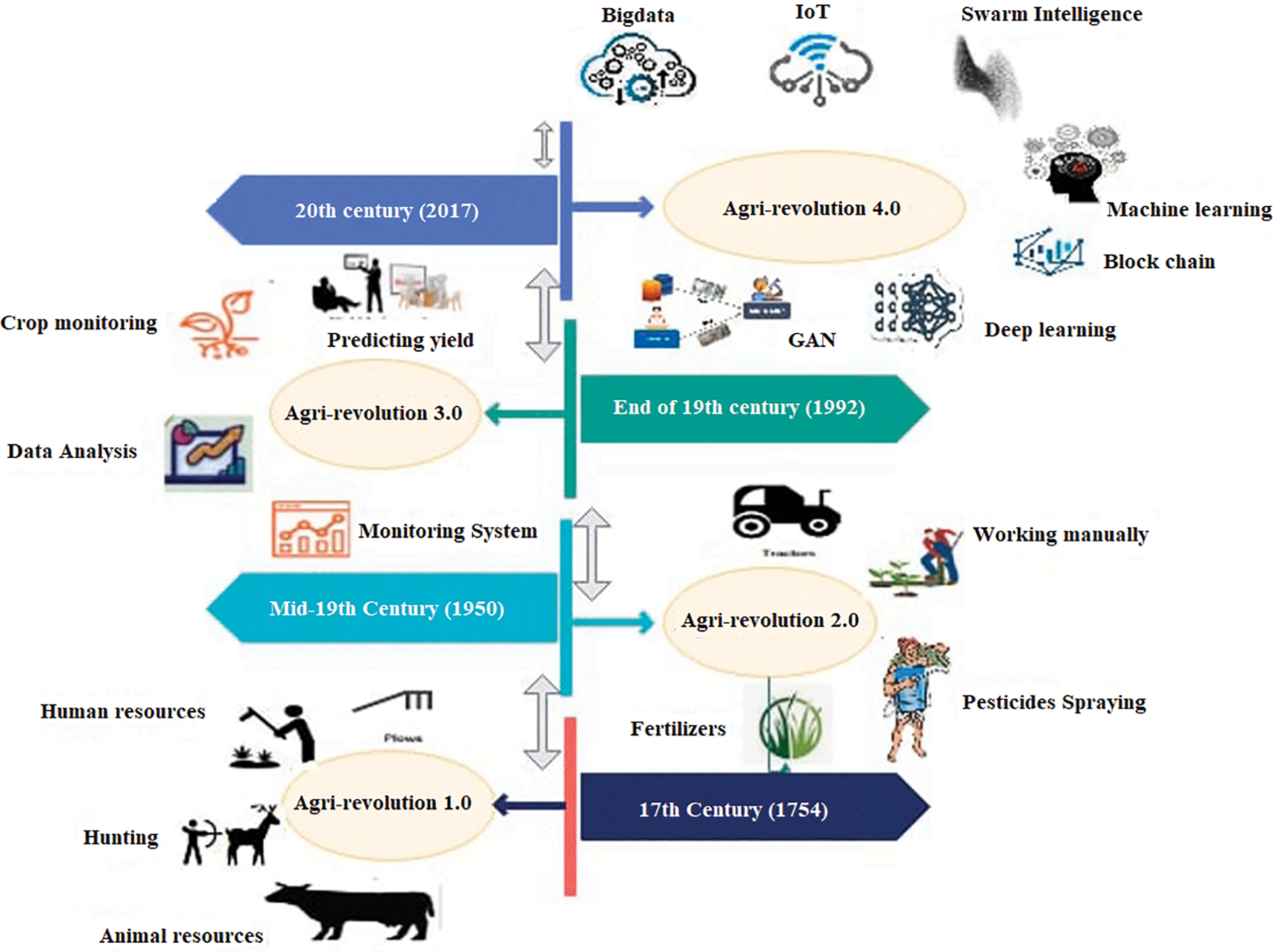
Figure 1: Road map of the agri generation 1.0–4.0 [10]. Adapted with permission form ref. [11], copyright © 2022
Agriculture 4.0 has just seen a new revolution due to computer vision. Scientists are developing computer vision systems for automated illness diagnosis [4,5]. Machine Learning, Data Science, Deep Learning, IoT [6–8], and blockchain [9] are just a few of the technologies described above that deal primarily with data and are extremely helpful for comprehending and offering fantastic insights into data. In order to gain insights into crop growth as well as aid in decision-making, these cutting-edge technologies are cast off in numerous agricultural practices, like choosing the finest crop for a given location and classifying elements that would rescind the crops, like insects, weeds, as well as crop diseases. Soil preparation, land management, water monitoring, weed identification, pesticide recommendation, spotting damaged crops, and cost calculation are the seven critical agricultural phases. Monitoring physical factors, such as weather and geological properties, is called land management. This is crucial since different climatic conditions exist all across the world and might have an impact on crops.
The unpredictable nature of rainfall, a significant component of the earth’s climate, directly affects biological, water management, and agricultural systems [12]. So that crop management may be made simpler, methods that help estimate rainfall in advance are needed. A vital part of agriculture is the soil. Soil depth affects a range of factors, including anchoring, anchoring, storing moisture and nutrients, mineral reserves, anchoring, and rooting [13]. Testing the soil is the first stage in the preparation of the soil. It entails determining the soil’s existing nutrient stages as well as the appropriate quantity of nutrients fed to a particular soil depending on its productiveness and the requirements of the crop. A variety of essential soil factors, including potassium, phosphorus, organic carbon, nitrogen, boron, as well as soil ph, are being categorized using the results from the soil test report [14]. Agriculture that uses Irrigation is crucial to soil and water conservation. Complex data may be employed to preserve irrigation performance as well as consistency when evaluating systems concerning soil, water, climate, as well as crop facts [15].
Plants that are growing where they are not wanted are known as weeds. It contains non-intentionally seeded plants. Crop yields are decreased by weed competition for nutrients, water, light, as well as space with agricultural plants. Reduce the quality of farm goods, resulting in irrigation water loss and making harvesting machines more challenging to operate. More about the crucial parts of today’s smart agriculture, including the production cycle, process, and supply chain.
And most importantly, the current state and significant discoveries of smart agriculture are discussed. Using the data in Fig. 2 Adapted from [10] shows the intelligent agricultural field works. Weeds and pests may reduce the economic value of agricultural areas. Farmers regularly spray standardized pesticides over the field twice throughout the growing season to suppress weeds and pests. However, this approach has led to excessive herbicides, which are bad for the environment, non-target animals, and people [16]. Plant diseases significantly reduce the quality as well as quantity of agricultural products and have a disastrous impact on food safety. In extreme cases, plant diseases may completely preclude grain harvesting.
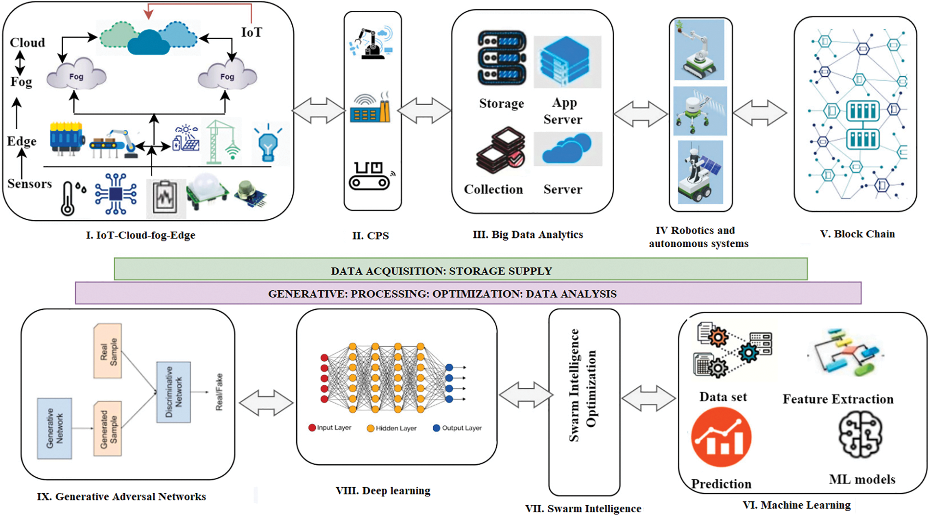
Figure 2: Smart farming technologies [10]. Adapted with permission form ref. [11], copyright © 2022
There are several reasons why a machine-learning-based approach for crop recommendation, plant seedlings, pests, and plant leaf disease detection can be highly motivating:
• Improved crop yield: Crop recommendation systems that utilize machine learning algorithms can analyze a range of data, including soil and climate conditions, to suggest the most appropriate crops for a given area. This can lead to more efficient use of resources and higher crop yields.
• Early detection of plant diseases: Identifying plant diseases early can help farmers take the necessary steps to prevent the spread of the disease and minimize the impact on crop yields. Machine learning-based systems can detect plant diseases from images of leaves and provide a quick diagnosis.
• Reduced pesticide use: Pest detection systems can help farmers identify pest infestations before they become severe. By catching infestations early, farmers can target only the affected areas and minimize the use of pesticides, reducing the environmental impact and saving costs.
• Increased efficiency: Machine learning-based systems can automate time-consuming tasks such as manual inspection of seedlings and plant leaves, freeing up time for farmers to focus on other aspects of their operations.
• Overall, using machine learning in agriculture can improve the efficiency and sustainability of farming practices, leading to better crop yields, lower costs, and reduced environmental impact.
Therefore, the steps involved in crop cultivation are the main emphasis of this work. It employs Deep Learning and Machine Learning algorithms to overcome numerous difficulties during cultivation. It primarily focuses on making crop recommendations based on weather factors. Additionally, it aids in the detection of pests, illnesses, and weeds. Following is a concise summary of the paper’s key findings:
• This study suggests a novel combination of improved SVM-RBF and Inception-V3 for Weed, insect, and plant leaf disease identification, as well as crop recommendation. It is easy to build, has a big impact, is extremely precise within a very small margin, and works well for problems involving search space optimization for small and large collections of characteristics.
• The optimum feature subset from the original dataset has been chosen using CNN-SVD, which prioritizes relevance over redundant and uninteresting traits.
• The CNN-SVD with an upgraded IV3 approach has not yet been tested or developed for detecting weeds, pests, and plant leaf diseases. As a result, a special combination method based on CNN-SVD-IV3 ought to greatly improve detection accuracy.
• Considering several indicators is a crucial part of this method for crop recommendation and detecting weeds, pests, and plant leaf diseases. The proposed feature selection method is assessed using the CNN-SVD. Results are validated using accepted clinical validation techniques.
After the introduction section, the article’s structure is as follows: Section 2 provides the prior relevant literature. Section 3 explained the layout and various aspects of the proposed strategy. Section 4 presents the experimental results along with a detailed explanation. Lastly, we finalized the study summary and areas of its implications are presented in Section 5.
The use of machine learning (ML) and deep learning (DL) has become essential in modern agriculture due to their ability to process large and complex data sets and make accurate predictions and decisions. Depending on the nature of the investigation, these models may be either descriptive or predictive. Explanatory models are used to forecast the future, while predictive models are used to glean insights from the data. Multiple machine-learning models have been presented in published works. To tackle the difficulties of smart farming, high-performance models are needed, considering several elements, including data diversity, soil quality, environmental conditions, and demographics [17,18]. Several studies have used machine learning approaches to assess yield prediction for crops, such as mustard and potato, by examining soil properties and using agronomic algorithms. Support vector machine (SVM) outperformed the decision tree method in terms of accuracy, with a score of 92%, and crop recommendations were made to the user using various algorithms, such as K Nearest Neighbor, Decision Tree, Linear Regression model, Support Vector Machine, Naive Bayes, and Neural Network algorithms [19,20]. However, using only two models will not provide the necessary results, as the production value predicted by these algorithms was under 90%. To address this, a suggested method uses web scraping to obtain temperature and humidity information, allowing for a user-interactive online interface that automatically retrieves and feeds information into an optimal model consisting of ten algorithms with hyperparameter adjustment. Compared to previous work, the suggested approach attains 95.45% accuracy by hyperparameter adjusting the algorithms [18,21,22].
Similarly, deep learning has attracted significant interest in smart farming due to its ability to extract high-level characteristics from raw data. Convolutional neural networks have been used to identify weeds growing alongside soybean, allowing for the accurate identification of weeds in agriculture fields. The suggested approach includes crucial skip and identification layers since it employs a pre-trained model like Resnet152V2, ensuring accurate forecasts. Additionally, experiments were done utilizing image features and machine learning methods to identify agricultural insects accurately. Compared to conventional insect identification, the CNN model achieved maximum classification rates of 90% and 91.5% [23–26].
Overall, there is a considerable demand for computerized crop recommendation and plant disease detection and diagnosis in agricultural informatics. Both machine and deep learning methods have emerged as the best solution due to their outstanding performance. This study primarily focuses on identifying crops depending on meteorological factors and outlining nutritional needs, aiding in Weed, pesticide, and disease detection. Finally, an efficient system is developed to help farmers choose the crop according to soil characteristics, detect weeds and pests, and diagnose diseases quickly [27,28].
This study proposes a unique methodology for improving the development of Machine Learning-based Agri-Food 4.0 via crop recommendation, weed identification, pesticide recommendations, and plant disease detection. The soil fertility, as well as crop friendliness detection and monitoring system, is applied at the initial stage, utilizing machine and deep learning methodologies to propose the correct crops cultivated in that soil. After recommending the appropriate crops, deep learning frames are created to identify undesirable development of weeds, pests, and diseases to improve crop growth. Fig. 3 shows the complete two-stage architecture of the proposed system.
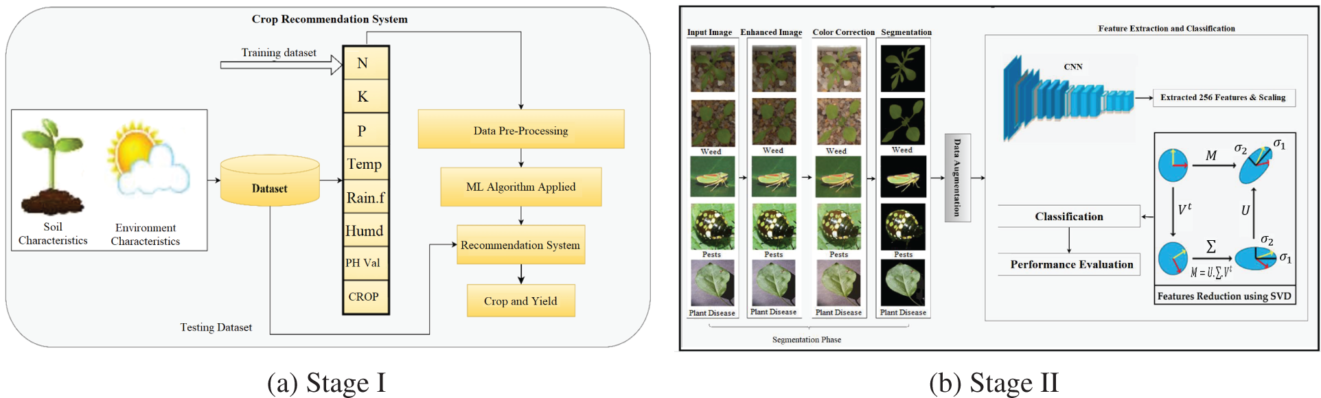
Figure 3: Proposed methodology
3.1 Stage 1: Crop Recommendation
Precision agriculture is currently popular. It enables farmers to make well-informed choices in farming strategy. This dataset allows users to create a prediction model that recommends the best crops to cultivate on a particular farm depending on numerous criteria. Augmented India’s existing rainfall, climate, weather, and fertilizer records for India created this dataset. New agriculture methods and processes are being developed, and procedures are being made in agriculture to combine cost-effective impacts, reduce downtime, and boost crop productivity.
However, gathering such vast amounts of data in agriculture is not a fundamental objective. Soil samples are collected and analyzed based on temperature, moisture, and humidity [29]. Specific libraries must be loaded in order to use ML algorithms and preprocessing tools. Model construction and prediction might be conducted effectively using these libraries. Pandas, NumPy, pickle, seaborn, matplotlib, Label Encoder, and train test split libraries were imported. On the soil dataset collected from Kaggle, the tests in this study are carried out utilizing the techniques of Logistic Regression, Nave Bayes, Decision Tree Classifier, Extreme Gradient Boosting (XGBoost) Classifier, Random Forest Classifier, Support Vector Machine (SVM), and K-Nearest Neighbors (KNN) [30]. These algorithms are used to assess the accuracy of the datasets. Fig. 4a depicts a portion of the crop recommendation dataset. Temperature, humidity, rainfall, nitrogen, potassium, and phosphorus vary per crop. Fig. 3 depicts the phases in the proposed study, including data preprocessing, model construction, as well as recommendations.
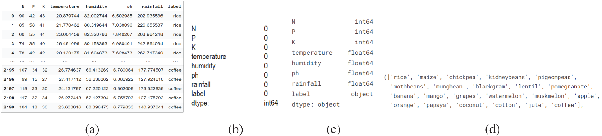
Figure 4: (a) Crop recommendation dataset (b–d) dataset attributes
A. Exploratory Data Analysis
Descriptive analytics will be used to find the optimal prediction model. Descriptive analytics offers an understanding of how the dataset appears and aids in discovering additional insight. Missing values for each attribute are verified when the dataset is imported. The crop recommendation dataset characteristics are free of missing values (b) datatype (c) the dependent variable, such as Label attribute (d), are shown in Fig. 4.
Once the key features of the dataset have been gathered, data visualization is used to assess the dataset visually. A correlation matrix is a table-like connection lattice describing the properties’ correlation coefficients. The characteristics are handled in this example’s first line and first column. Fig. 5a depicts the dataset’s correlation matrix. The dispersion of crop examples in the dataset is depicted in Fig. 5b. The Figure indicates that all crops in the dataset are spread evenly. Each character in the dataset, such as the Label column, is plotted against the dependent variable.
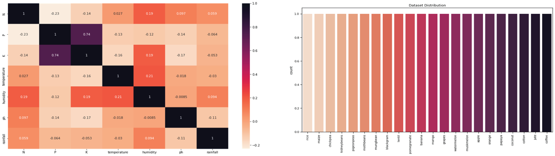
Figure 5: (a) Dataset correlation matrix (b) crops distribution
The report states that cotton needs more nitrogen for growth than all other crops regarding nitrogen requirements per crop; Fig. 6 provides these specifics (a). Similarly, (b) defines the Potassium demand for each crop, with grapes and apples having the greatest requirements and orange consumption having the lowest, followed by (c) identifying the Phosphorous required for each crop, with grapes and apples having the highest requirements. Regarding temperature requirements for each crop, papaya demands the highest temperature, as shown in (d). Coconut requires more humidity than other crops, while rice requires more rainfall than all other crops, as shown in (e), (g). When assessing the soil Ph needed per crop, practically all crops require a higher Ph value, as shown in (f).
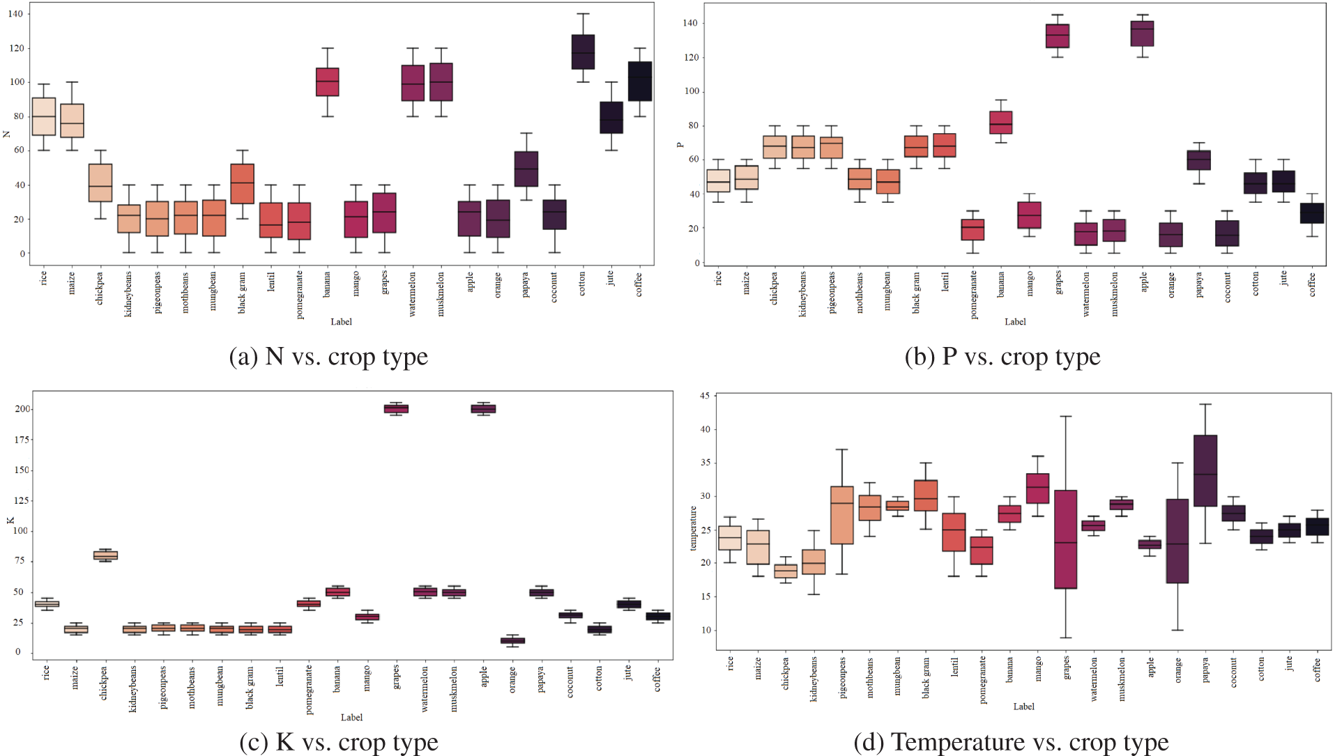
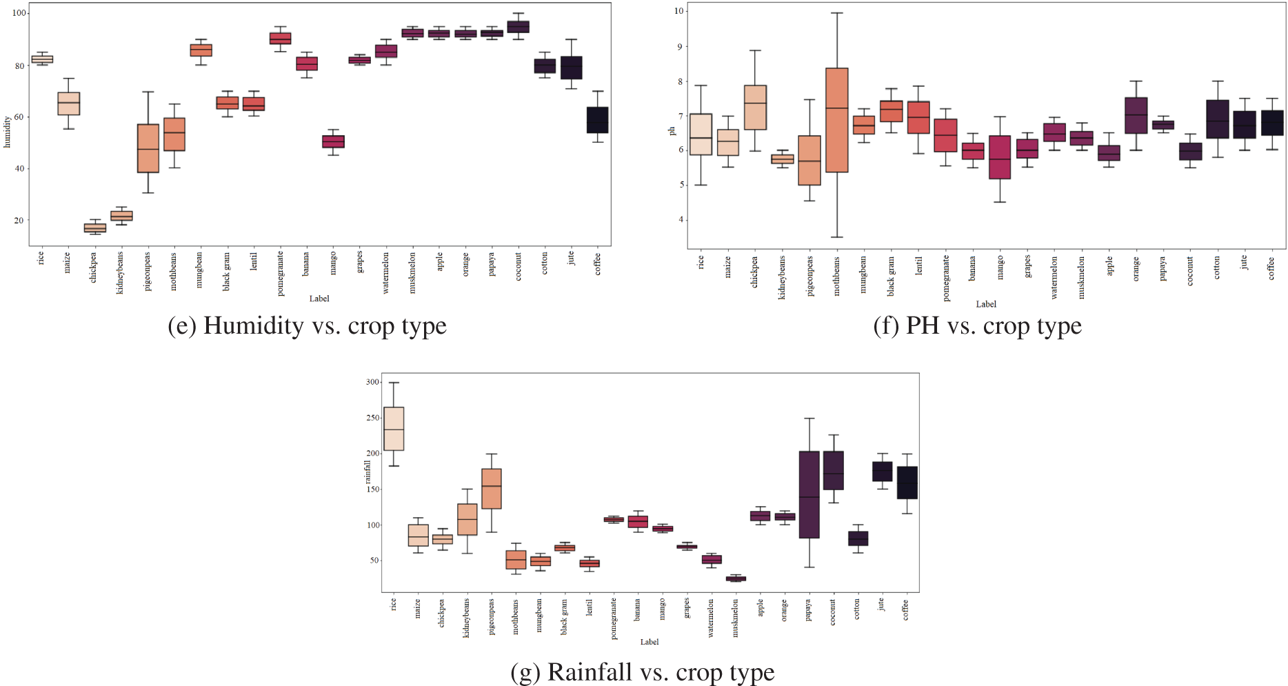
Figure 6: Condition requirements for each crop
Except for the Label element, all of the characteristics are numerical. Distribution plots are often used for univariate data sets and display information as a histogram. As a result, distribution plots were created to determine the data distribution throughout the dataset. The value of a Phosphorous is not evenly distributed in Fig. 7. Concerning Fig. 7, the potassium column shows more zero values. In Fig. 7, which depicts the Nitrogen data distribution, values range between 20–45 and 75–120. Fig. 7 illustrates the data distribution for the Temperature Column. The majority of the values fall between 20 and 35. It also depicts the data’s normal distribution. The values in rainfall are not evenly distributed in Fig. 7. In figure, the values for the soil Ph column are more evenly distributed throughout the range of 5.5 to 7.5. The distribution graphs show that the data in each column is not normally distributed, and the value counts change between ranges.
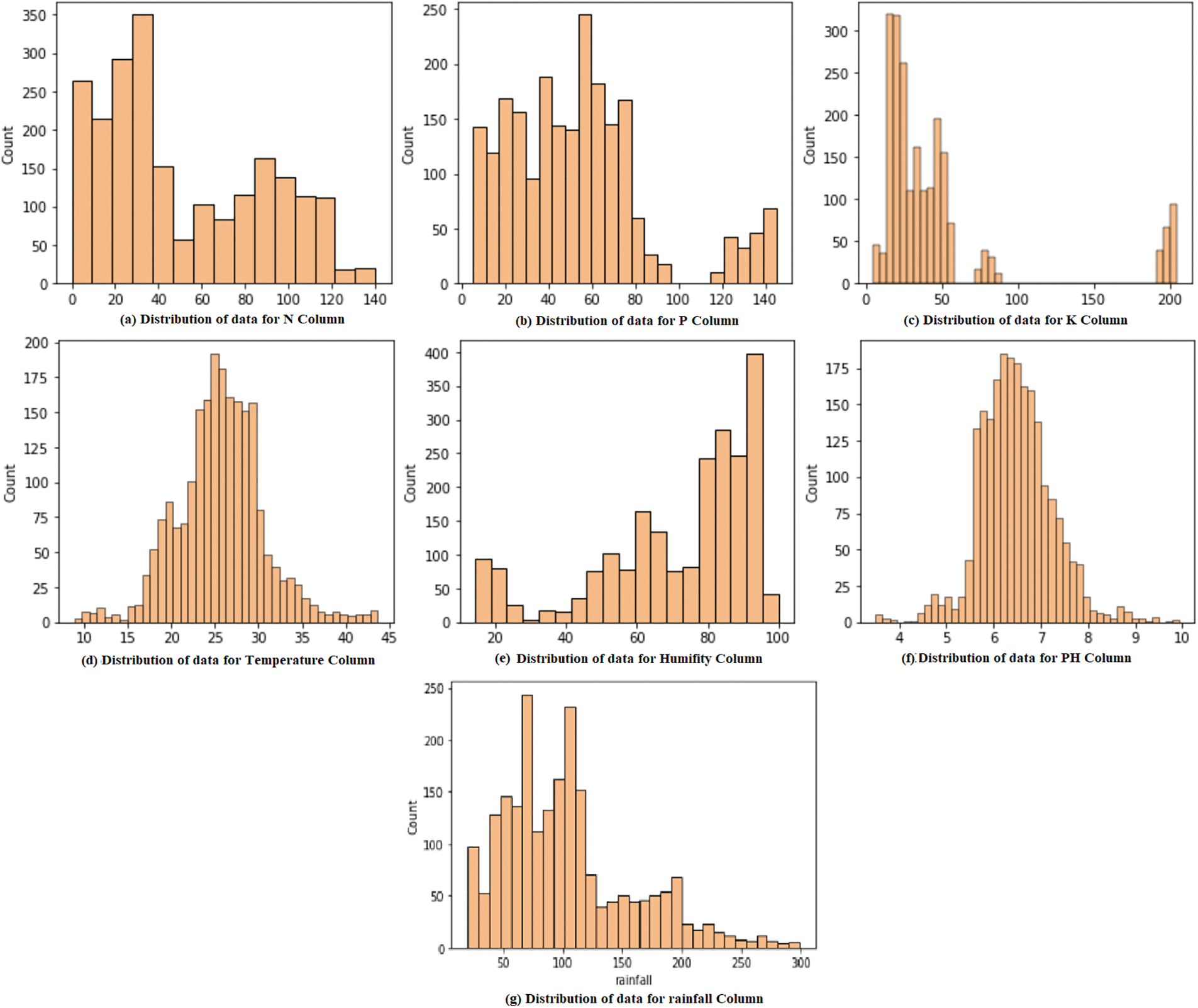
Figure 7: Distribution of the data
This study discussed novel AI prediction modules for predicting the best crop. This module was built with the Keras deep learning neural network. The Google Colab platform is utilized to create the model, and classes and methods from important libraries such as Scikit-learn, Numpy, and Pandas are loaded and imported. Training data is the first data necessary for training machine learning algorithms. To learn how to produce accurate predictions or to perform the desired task, machine learning algorithms are fed training Datasets. A testing set is a data collection used to evaluate a finished model fit on the training sample correctly.
3.1.3 Performance Evaluation Metrics
The height of correctness is estimated by understanding and specificity assessments. The presentation assessment measures consumed in the recorded learning are listed below:
Accuracy: This is the ratio of a classifier’s precise prediction produced by a classifier when equated with the label’s actual value during the testing stage. Also known as the ratio of correct evaluations to total assessments. Use the following Eq. (1) to assess accuracy.
F1-Score indicates the harmonic mean value of recall and precision, as stated in Eq. (2).
Precision: Precision is a critical characteristic to consider while evaluating precision. It indicates how many positive cases the classifier identified from the number of predicted positive examples provided in Eq. (3).
Recall: The proportion of positive samples recognized as positive by the classifier is determined by recall. When there is a significant cost coupled with False Negative, the recall is a performance parameter used to choose the optimal model, as stated in Eq. (4).
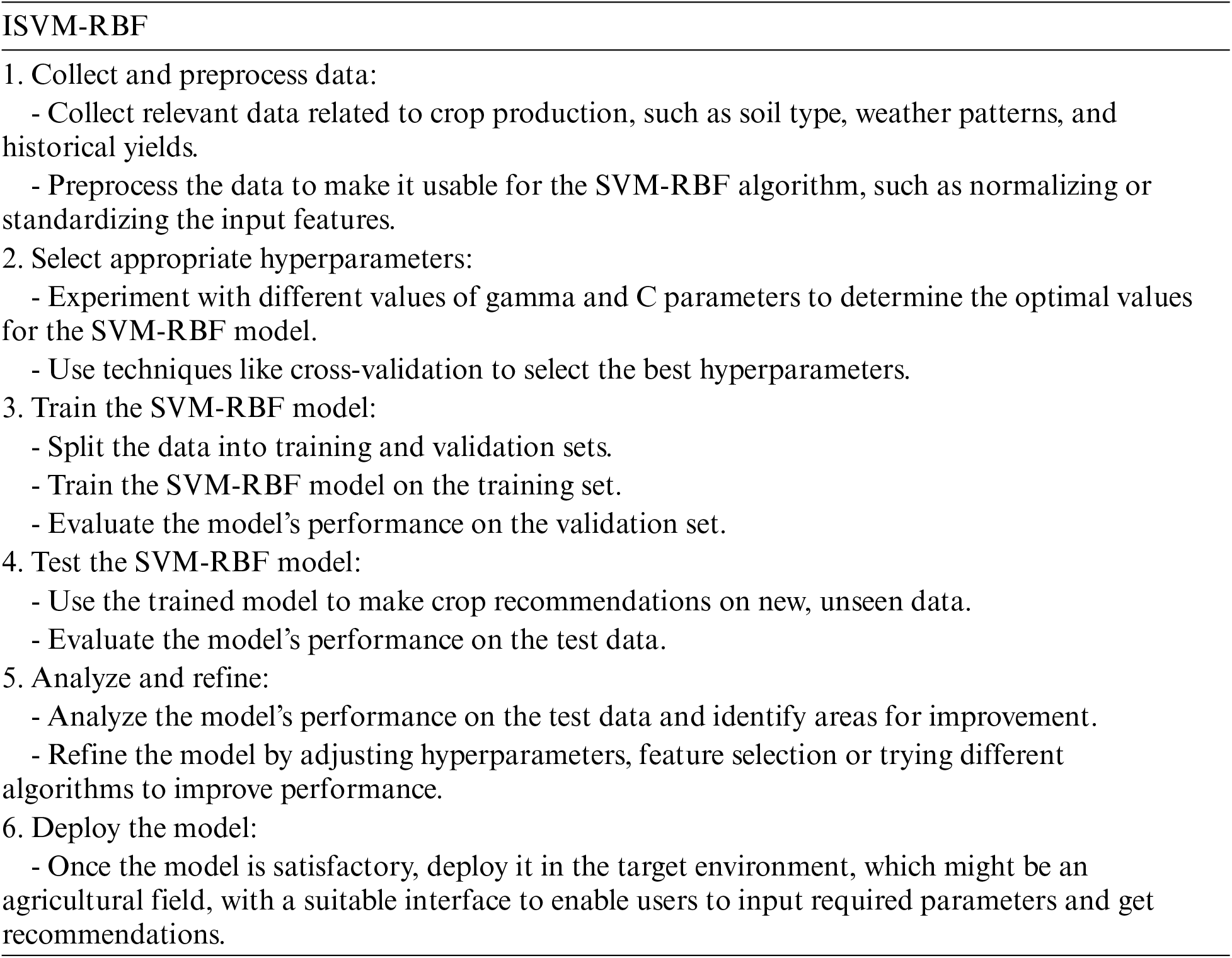
3.1.4 Classification Using Novel ISVM-RBF
The new ISVM-RBF is defined as aggregation variations that may be utilized for regression and Classification. The ISVM-RBF is non-parametric, unlike conventional statistic-based parametric classification methods. Although the SVM is among the most widely used non-parametric ML procedures, it loses performance with several data samples. As a result, the new ISVM-RBF increases the efficiency and accuracy of change detection. Furthermore, they do not need any assumptions about data distribution. A non-linear ISVM-RBF utilizes functions to reduce the computational burden when the data cannot be classified as linear or non-linear. This is known as the kernel trick. Popular methods include polynomial kernel and Gaussian kernel.
Furthermore, in the non-linear separable condition, the SVM-RBF maps input variables to a high-dimensional feature space using a pre-selected non-linear mapping function, building the best classification hyperplane in the space. The SVM-RBF Variants will discover a hyperplane with the same properties as the straight line in the preceding example. Four kernel functions are widely employed, but we enhanced and only utilized the radial basis function variations in our study, also known as the Gaussian variants.
As a result, the improved ISVM-RBF includes
where
The SVM-RBF may integrate binary classifiers using the one vs. all (OVA) method. The one against all approach generates one binary classifier for each class in a
3.2 Stage 2: Weed, Pests, and Plant Leaf Disease Detection
To evaluate the effectiveness of the proposed methods, we use the plant seedlings dataset [31] for weed identification, IP102 [32] and D0 [33], two publically available datasets are used for pests Pest Classification in the end plant village dataset [34] is used for plant leaf disease detection. In this section, we conduct an exploratory analysis of the databases used to compile this study.
The plant seedlings dataset from Kaggle was utilized for this module, as shown in Fig. 8 [31]. This dataset was used since it contains photographs of several phases of weed development. This is critical since it has photos of all weed stages. Any weed in its early stages may be photographed and entered into the system. The suggested study effectively classifies the weed kind. This is because the model was trained using the planting dataset.
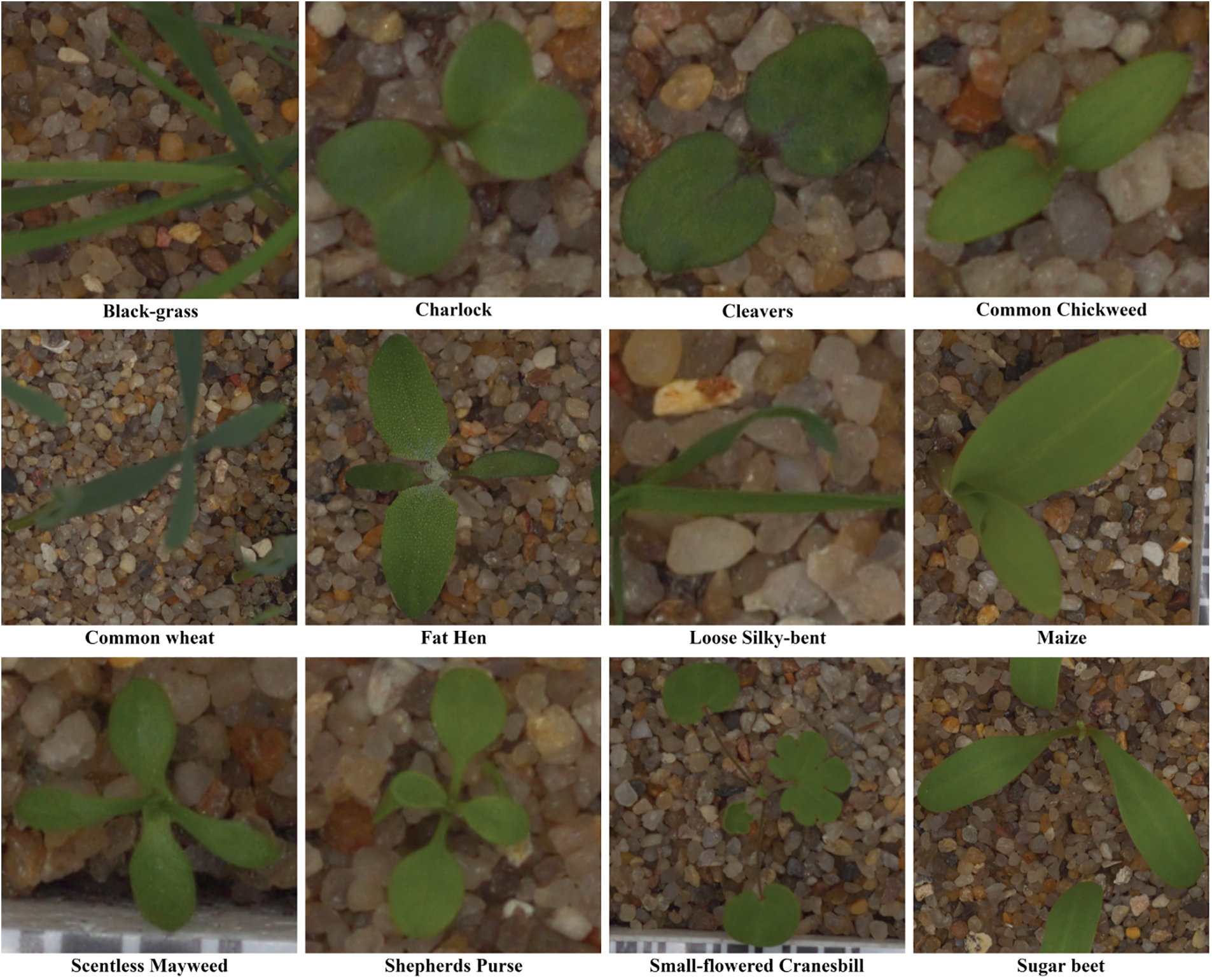
Figure 8: Plant seedling dataset samples
3.2.3 Pests Identification Datasets
• The IP102 [32] dataset comprises almost 75,000 photos divided into 102 categories. It has a natural long-tailed distribution. Furthermore, we annotate 19,000 images with bounding boxes to aid object recognition. The IP102 has a hierarchical taxonomy, and insect pests that mainly harm one agricultural commodity are classified together at the top level. Fig. 9 shows several photographs from the IP102 dataset (a). Each picture depicts a different insect problem species.
• D0 [33] includes 4500 pest photos covering most species present in common field crops, such as maize, soybean, wheat, and canola. Most of these pest pictures were obtained under real-world situations at the Anhui Academy of Agricultural Sciences in China. There are 40 pest species in the pest dataset (D0). Fig. 9 depicts some sample photos (b). All photographs were taken with digital cameras (e.g., Canon, Nikon, and mobile devices). All sample photos were preprocessed in crop field circumstances with consistent illumination settings to remove the possible detrimental impacts of light variability. Furthermore, for computational efficiency, they were normalized as well as rescaled to 200 By 200 pixels in this study. The collection of photos for each bug species was randomly divided into two subsets: the training set of around 30 images as well as the test set with the remaining pest images.
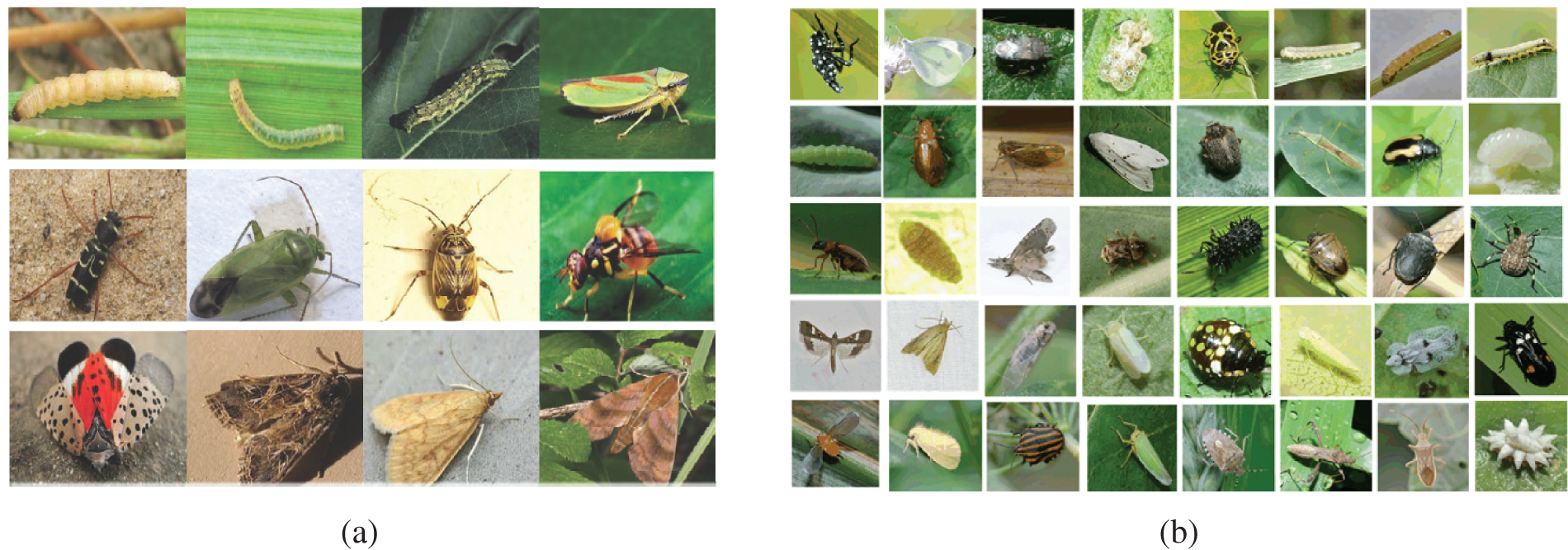
Figure 9: Example images (a) IP102 dataset, (b) D0 from the field-based pest collection dataset
3.2.4 Plant Leaf Disease Dataset
The PlantVillage dataset [34] is a free, open-access database with over 50,000 photos of healthy and damaged crops with 38 class labels. We chose photographs of healthy apple leaves and images of black rot produced by the fungus Botryosphaeria obtuse on apple leaves. Botanists classify each picture into one of four categories: healthy, early, medium, or end-stage. The leaves in the healthy stage are spotless. Small circular patches with widths less than 5 mm can be found on early-stage leaves. More than three frog-eye spots enlarge to form an uneven or lobed shape on the middle-stage leaves. The dying leaves are so diseased that they will fall from the tree. Agricultural specialists assess each photograph and identify it with the proper disease severity. One hundred and seventy-nine photos are eliminated due to expert disagreement. Fig. 10 depicts several instances of each step. Finally, we have 1644 photos of healthy leaves, 137 photographs of early-stage illness, 180 images of middle-stage disease, and 125 views of end-stage disease.
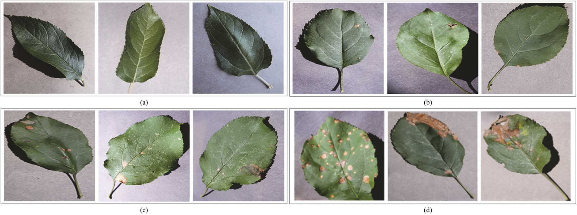
Figure 10: Plant village dataset sample images
3.3 Preprocessing and Data Augmentation
Preprocessing improves the provided fundus picture by performing adaptive histogram equalization with contrast stretching, followed by a median filtering approach. The preprocessing stage is completed in the brightness, chroma blue (CB), as well as chroma red (CR) color spaces of the fundus image. Consequently, it adds two of the Red, Green, Blue (RGB) chromatic color components to the intensity (Y), yielding the YCbCr picture (transformation of RGB image to YCbCr image). The Y component is extracted from the YCbCr picture to perform the median filtering procedure. Following that, the contrast may be stretched, and the intensity normalized. The image is after that converted to RGB using the inverse transform of YCbCr.
Avoiding overfitting as well as generalization problems is considered one of the most fundamental characteristics for the efficient processing of AI models. The distribution of the dataset across grades is considerably skewed, with the bulk of photos coming from grades 0 and 2. This highly unbalanced data set could lead to a wrong classification.
We used data augmentation methods to enlarge the FI dataset at various scales. Listed below are the key data augmentation processes that we implemented.
• Rotation: Images revolved at random from 0–360 degrees.
• Shearing: Sheared with an angle randomly ranging between 20 and 200 degrees.
• Flip: Images were flipped in both the horizontal and vertical directions.
• Zoom: Images were extended randomly in the (1/1.3, 1.3) range.
• Crop: Randomly selected images were scaled to 85% and 95% of their original size.
• Translation: Images randomly shifted between −25 and 25 pixels in both directions.
In this section, we have planned on using a fundamental CNN to gain the greatest number of significant features. The model’s classification performance will be enhanced if the fundamental properties that differentiate between the various stages are extracted. That's why we used a basic CNN model. The CNN feature extractor is laid out in Fig. 11, which shows its configuration.
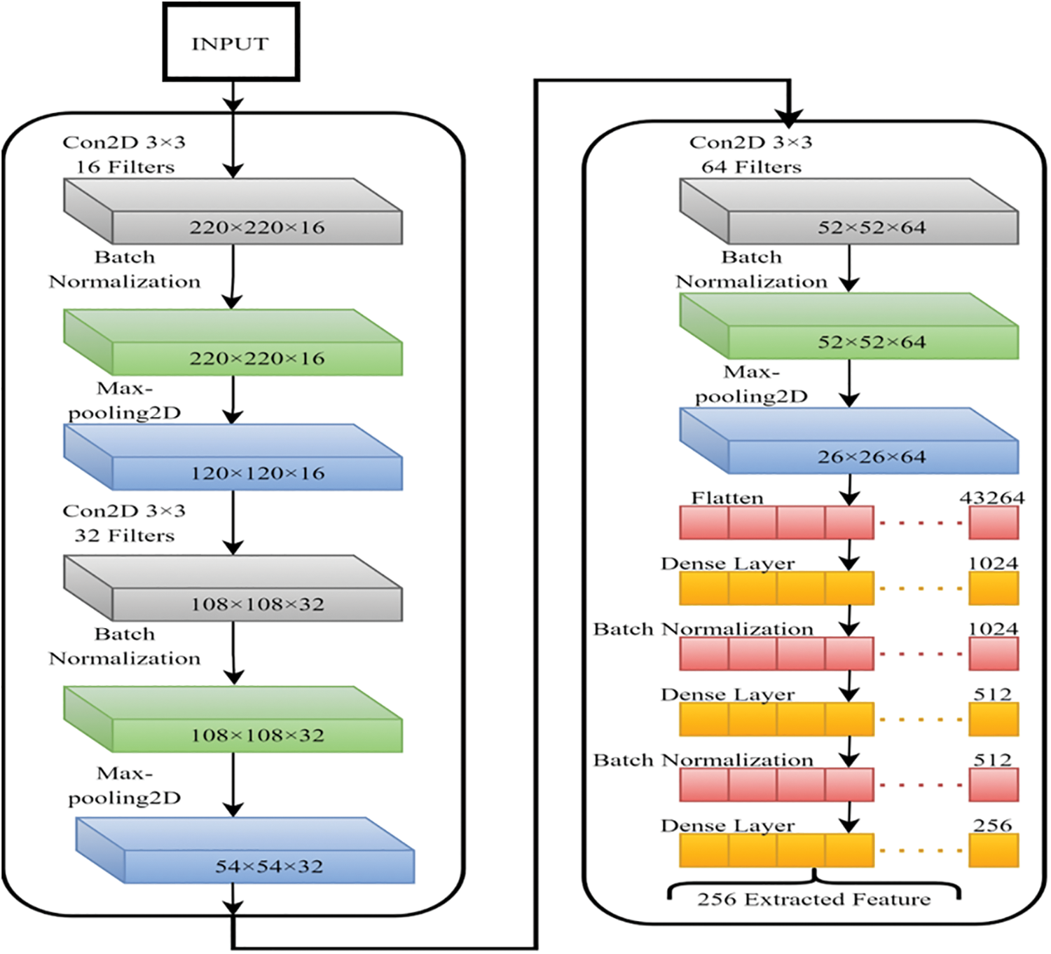
Figure 11: CNN model for the features extraction
These generated features are capable of being used efficiently for Classification. Every CNN convolutional layer has been treated with batch normalization along with a max-pooling layer. The use of batch normalization was decided upon because this technique accelerates the modeling process and improves its overall performance by re-centering and re-scaling the inputs of the various layers [35]. The most important value from every neuron in a cluster is selected using Max-polling to extract the relevant characteristics from the treated images [36,37]. In this case, dropout avoids overfitting by skipping training nodes for each layer, speeding up the training process. Adam was an optimizer due to his exceptional performance with big data sets [38]. After that, the ultimate dense layer was employed to get 256 distinguishing attributes from every image.
The fundamental concept of Fast Fourier Transform (FFT) is the foundation for feature reduction by SVD. A matrix
Hence, STU* can be written as:
In order to convert D through optimal lower-rank approximations, SVD chooses the higher-valued components of T that are greater than a specific value from T. This allows D to be transformed into an optimal lower-rank approximation.
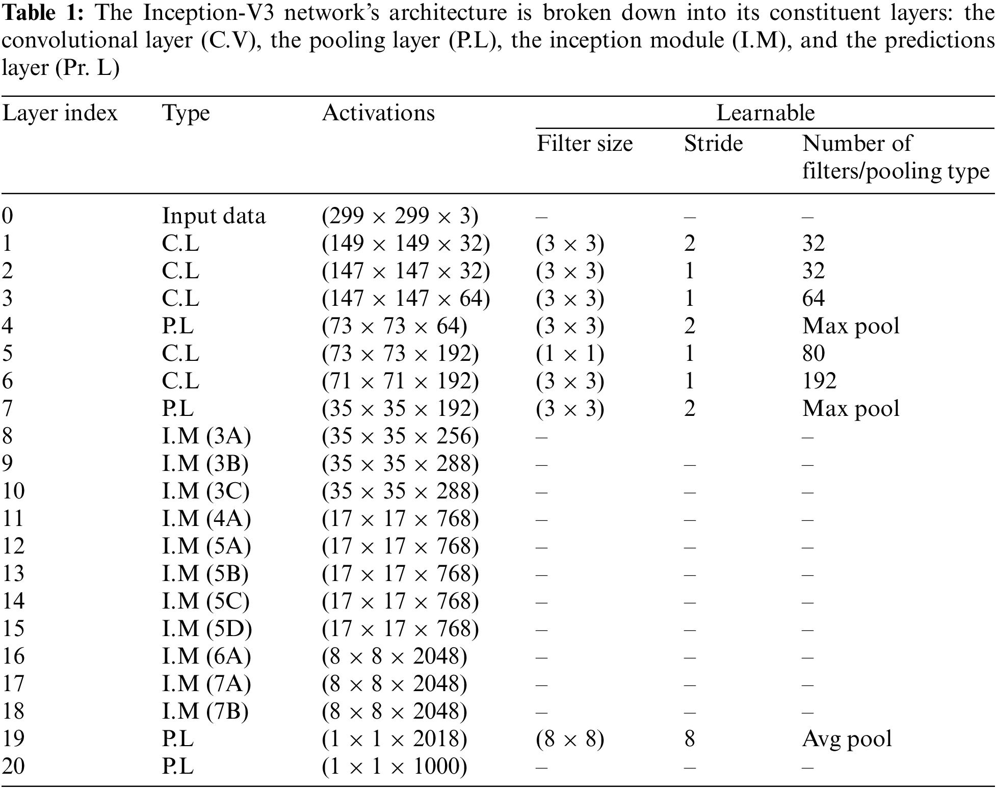
3.5 Classification Using an Improved Inception-V3
It’s a Deep Neural Network (DNN) that can sort through 1000 distinct types of objects for Classification. The model is first trained on a large dataset of photos, but it may later be retrained on a smaller dataset while retaining its original training data. One of the benefits of the Inception-V3 CNN model is that it may enhance classification accuracy without requiring extensive training, significantly decreasing processing time. Layers, activation functions, and the extent to which Inception-V3 is a learnable network are all laid out in Table 1. The Inception-V3 network’s principal goal is to eliminate the bottleneck representation between network layers, making the next layer’s input size much smaller. In order to reduce the network’s computational complexity, the factorization approach is used.
4 Experimental Results and Discussion
All tests were carried out in the Python programming environment. An Intel Core i7 8th generation CPU with 2 TB SSD memory and 16 GB of RAM was used. This section highlights the significant findings of the picture preprocessing, time complexity, as well as classifier results. A comparative analysis of the planned work to traditional approaches is also provided.
A comparison of different classifier accuracy with testing and training accuracies is presented in Fig. 12. Notably. The Support Vector Machine (SVM) algorithm using a radial basis function (ISVM-RBF) machine learning (ML) model performs better. Among all classifiers, Naïve Bayes, logistic regression, K-Nearest Neighbors (KNN), Decision Tree (DT), Support Vector Machine-Linear (SVM-L), Support Vector Machine-Polynomial (SVM-P), Random Forest (RF), and Extreme Gradient Boosting (XGBoost).
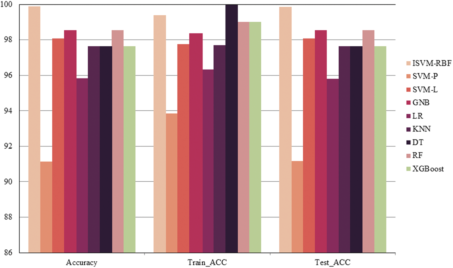
Figure 12: Accuracy comparison
ISVM findings are shown in Figs. 13a–13i. The predicted values of the testing set are shown as a list, preceded by the training and test set accuracy score with the accuracy score of that model for the crop suggestion dataset. The classification report displays the model’s accuracy, recall, and f1-score. The same processes are taken for each of the 11 algorithms to generate the appropriate predicted values, training set accuracy, testing set accuracy, and classification report. The confusion matrix for each classifier is also shown in Figs. 13a–13i. The diagonal of the confusion matrix indicates how frequently the forecast was right.
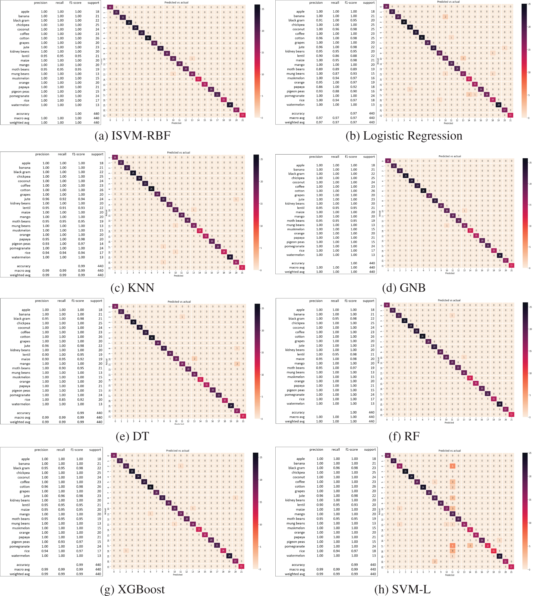
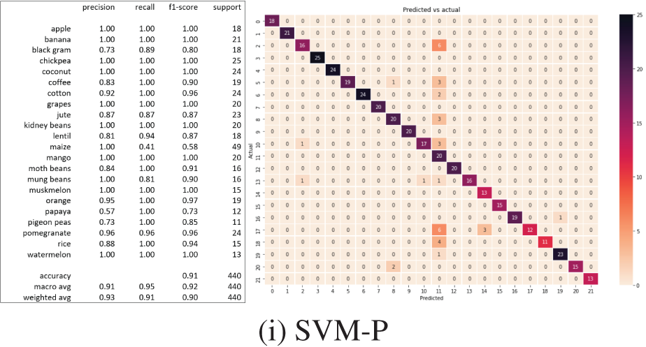
Figure 13: Classification results and confusion matrix
The user may give factors such as N-P-K, temperature, humidity, pH value, rainfall, and crop in the crop suggestion, and the program will predict which crop the user should grow.
4.2 Weed, Pests, and Plant Leaf Disease Detection
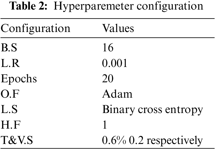
The outcomes of the suggested transfer learning-based system for Weed, insect, and plant leaf disease identification on the farm are highlighted in this section. The picture is utilized as an input for the CNN-SVD for feature extraction with transfer learning-based CNN models after it has been processed and segmented. The suggested methodology is tested on three public Weed, pest, and plant leaf datasets: Plant seedlings, Plant leaf disease, and Pest identification. To assess the three databases, tests were performed on six pre-trained models (Proposed-Inception-V3, ShuffelNEt, MobileNet, SVM, K-NN, RF). Our suggested strategy outperforms other earlier studies, according to the experimental data. All practical algorithms are written in Python 3.6 and use the TensorFlow/Keras package. Python is also used for picture preparation and augmentation. As shown in Table 2, the optimum hyperparameters are batch size (B.S), loss function (L.S), learning rate (L.R), target size (T.S), Taring and Validation Split (T&V.S), histogram_freq (H, F), and optimization function (O.F).
The suggested method results were compared to three well-known machine learning as well as two deep learning algorithms. Tables 3–6 show that the proposed technique outperformed ShuffelNet, MobileNet, SVM, K-NN, and random forest. A five-fold cross-validation test was used to assess the performance of experimental findings on the Plant seedlings, Pest identification, and Plant leaf disease datasets. Figs. 14a–14c demonstrate the training accuracy and loss of deep learning models for all datasets. In Fig. 14c, the training loss gradually diminishes after the seventh period.
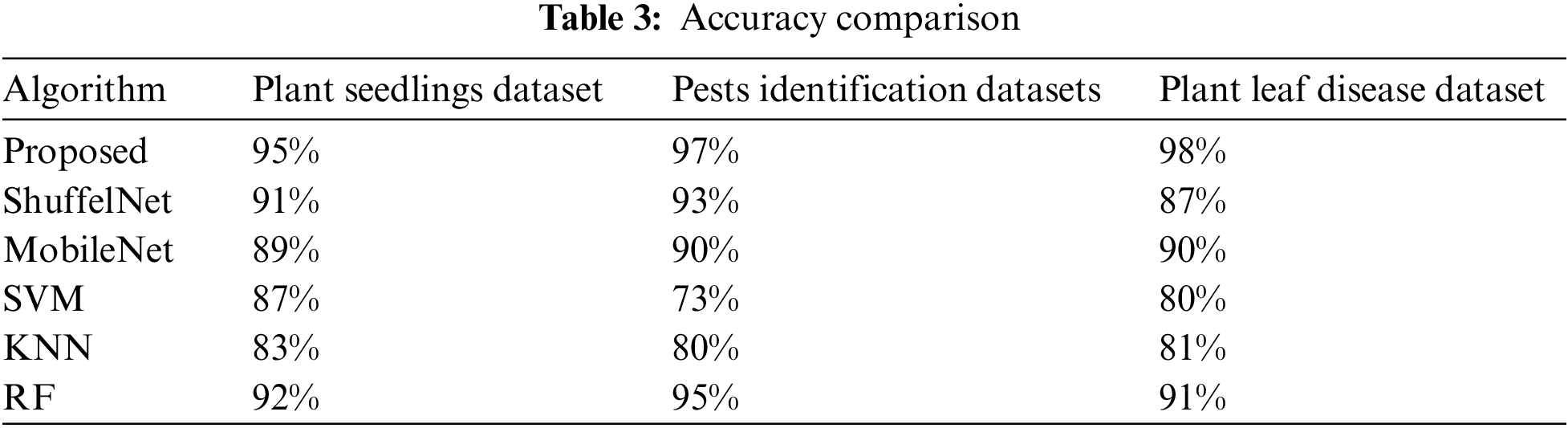
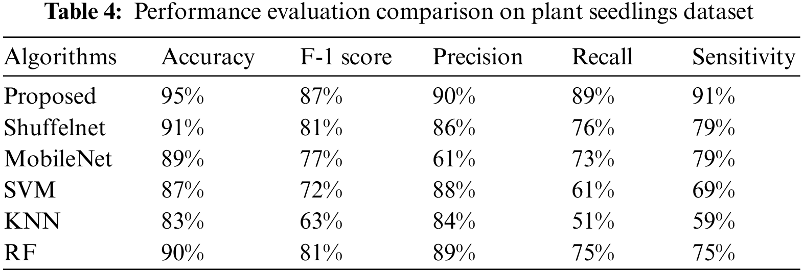
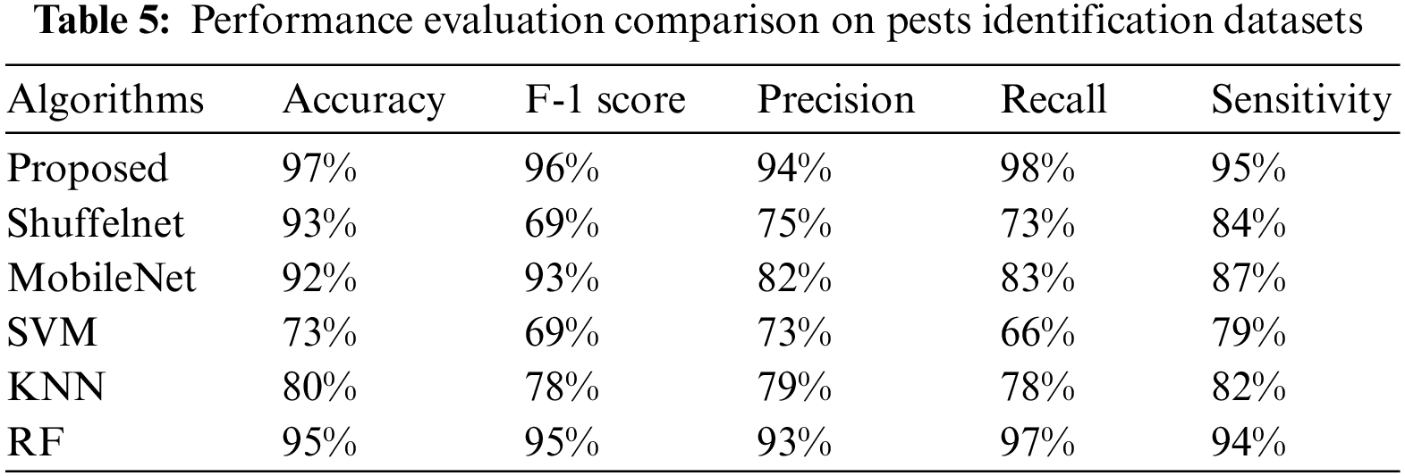
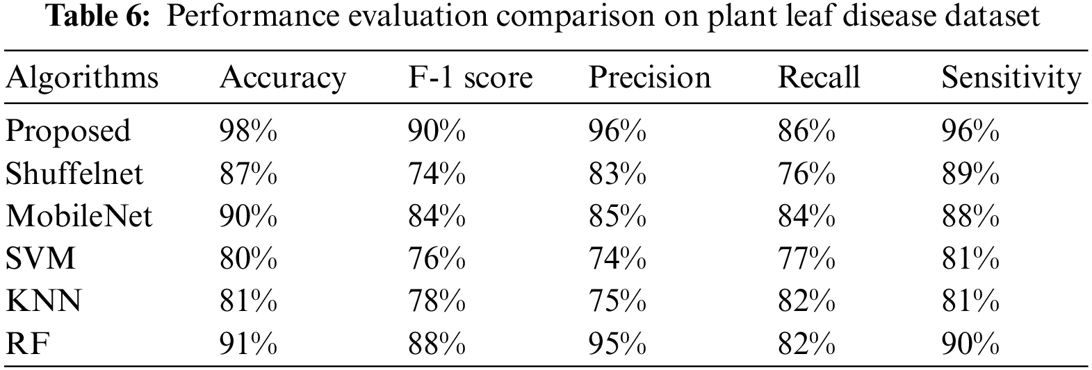
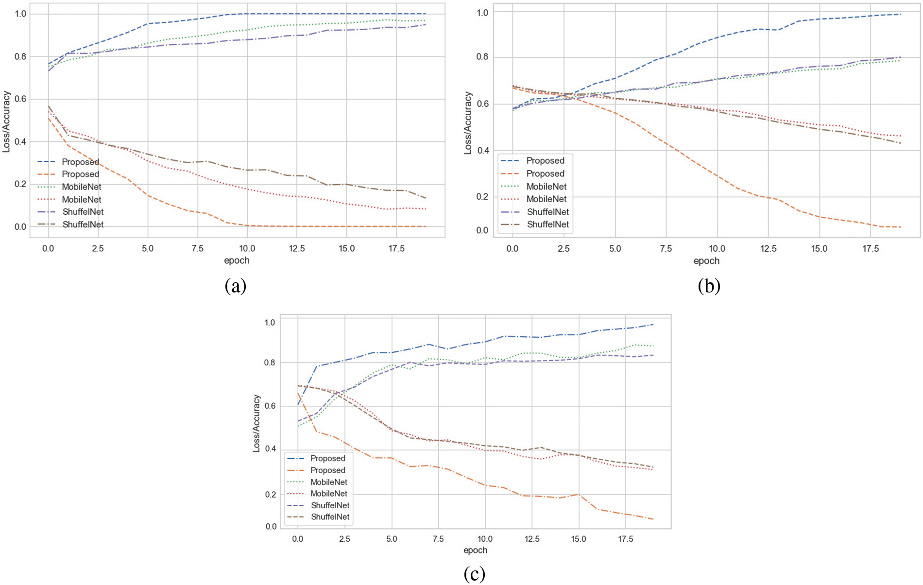
Figure 14: (a) Training accuracy and loss on plant seedlings dataset (b) training accuracy and loss on pests identification datasets (c) training accuracy and loss on plant leaf disease dataset
The training accuracy, on the other hand, remains consistent throughout iterations. The loss and accuracy of shuffelNet and mobile net are more diminutive, indicating that our model is ideally matched to the Plant seedlings dataset. Figs. 14a–14c show that after the 10th epoch, the training loss progressively reduces for the Pest identification datasets as well as Plant leaf disease datasets. In contrast to shuffelNet and mobile net, training accuracy stays greater until the last epochs. After the 17th epoch, the training accuracy on all datasets hit 99%, indicating that our model was regularized and perfectly fitted.
Table 3 shows that the suggested technique performed best, with accuracies of 0.95, 0.97, and 0.98 on the Plant seedlings, Pest identification, and Plant leaf disease datasets, respectively. ShuffelNet, MobileNet, SVM, K-NN, and RF accuracies on the Plant seedlings dataset were 0.91, 0.89, 0.87, 0.83, and 0.90, 0.93, 0.90, 0.73, 0.80, and 0.95, and 0.87, 0.90, 0.80, 0.81, and 0.91 on the Plant leaf disease dataset. The suggested technique outperforms ShuffelNet, MobileNet, SVM, K-NN, and RF on the Plant seedlings dataset, 4%, 7%, 24%, 17%, and 2% on the Pests identification dataset, and 11%, 8%, 18%, 17%, and 7% on the Plant leaf disease dataset.
Table 4–6 shows that the proposed technique achieved 87%, 90%, and 89% f1-score, precision, as well as a recall on the Plant seedlings dataset, 96%, 94%, and 98% on the Pests identification dataset, and 90%, 96%, and 86% on the Plant leaf disease dataset, which were greater than ShuffelNet, SVM, MobileNEt, K-NN, as well as RF, respectively.
Furthermore, the suggested strategy outperformed ShuffelNet, MobileNet, SVM, K-NN, and RF on the Plant seedlings dataset by 6%, 10%, 15%, 24%, and 6%, respectively. Furthermore, on the Pests identification datasets, f1-score was 27%, 3%, 27%, 18%, and 1% greater than ShuffelNet, SVM, MobileNEt, K-NN, as well as RF, and 16%, 6%, 14%, 12%, and 2% higher than ShuffelNet, SVM, MobileNEt, K-NN, as well as RF.
Furthermore, the accuracy and recall of the proposed model Plant seedlings dataset were 4%, 29%, 5%, 2%, 6%, 1%, 13%, 16%, 28%, 38%, and 14% higher, respectively, than ShuffelNet, MobileNet, SVM, K-NN, as well as random forest. The precision and recall performance of the proposed technique for the Pests identification datasets and Plant leaf disease dataset were 19%, 12%, 21%, 15%, 1% and 25%, 15%, 32%, 20%, 1% and 13%, 11%, 24%, 2%, 1% and 10%, 2%, 9%, 4%, 4% better than ShuffelNet, MobileNet, SVM, K-NN, and RF.
When comparing the sensitivity of the proposed model to ShuffelNet, MobileNet, SVM, K-NN, and RF on the Plant seedlings dataset and Pests identification datasets, the proposed model is 3%, 13%, 11%, 8%, 2%, 1%, 1%, and 16%, 13%, 1% greater, respectively, as shown in Tables 4–6. The sensitivity of the proposed method on the Plant leaf disease dataset was 7%, 8%, 15%, 15%, and 6%, respectively.
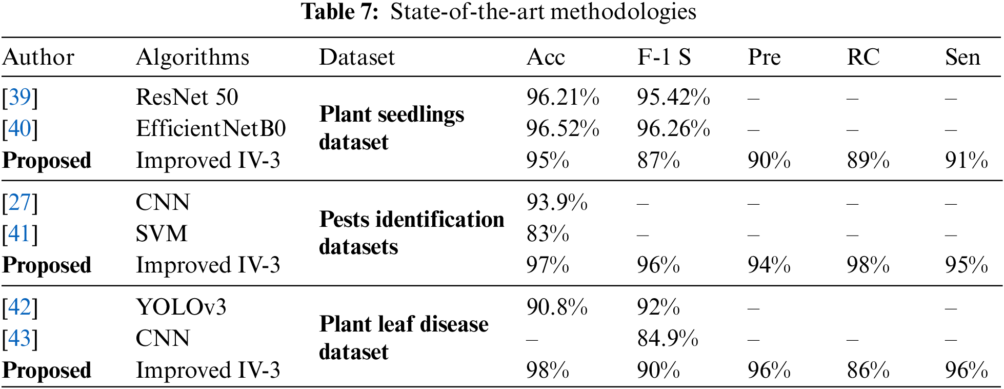
Table 7 compares the accuracy of the proposed ISVM-RBF approach with state-of-the-art methodologies.
A sustainable and resilient agricultural system is the future of farming. Currently, information is the key to efficient farming. However, new agricultural automation capabilities are hampered because of a lack of awareness about technological advancements. In addition, agriculture is considered the economic lifeblood of every nation. Therefore, prompt monitoring is required in this field. This manuscript proposed a novel two-stage framework to boost Agri-Food 4.0 development. In the first phase, we assess the current climate and environmental conditions to determine which crops should be irrigated and how much water each needs to produce its maximum yield. One who needs crop advice can use this as a reference instead of making mistakes through trial and error. Using machine learning technology, we have developed a model to assist farmers in selecting the most productive crop by considering environmental factors such as N, P, K, pH, relevant temperature and humidity, and precipitation. The second phase identifies weeds, corrects insects, and diagnoses plant diseases. This will help to recommend deciding which pesticides and herbicides to prescribe for similar situations.
In the future, we initially plan to propose a model that can be used to estimate the full financial outlay required for a certain cultivation effort. This would help in preparation for cultivation, leading to all-encompassing farming solutions. Many farmers have no idea how much it costs to grow their crops. There’s a chance the farmers will lose money because of all the uncertainties. It will also help fix estimates regarding cultivation costs, including labor (human and animal) and inputs (seeds, manures, and fertilizers). It will also provide guidelines on organizing your efforts and making farming profitable. Secondly, we’ll build an application for real-time crop recommendation, weeds, pesticides, disease detection, and cost estimation.
Acknowledgement: We would like to express our sincere gratitude to all those who have supported and contributed to the completion of this manuscript.
Funding Statement: This research was funded by the National Natural Science Foundation of China (Nos. 71762010, 62262019, 62162025, 61966013, 12162012), the Hainan Provincial Natural Science Foundation of China (Nos. 823RC488, 623RC481, 620RC603, 621QN241, 620RC602, 121RC536), the Haikou Science and Technology Plan Project of China (No. 2022-016), and the Project supported by the Education Department of Hainan Province, No. Hnky2021-23.
Author Contributions: The authors confirm contribution to the paper as follows: Conceptualization, A. B and H. L; Methodology, A. B, M. S, X. L and M. W; Software, A. B and M. S; Validation, A. B and M. W; Formal analysis, X. L, M. W; Writing—original draft, A. B; Writing—review & editing, M. S, X. L, M. S; Visualization, H. L, X. L; Project administration, H. L; Funding acquisition, X. L, H.L.
Availability of Data and Materials: The data used to support the findings of this study are available from the first author upon request.
Conflicts of Interest: The authors declare that they have no conflicts of interest to report regarding the present study.
References
1. J. Campolo, D. Güereña, S. Maharjan and D. B. Lobell, “Evaluation of soil-dependent crop yield outcomes in Nepal using ground and satellite-based approaches,” Field Crops Research, vol. 1, no. 260, pp. 107987–108002, 2021. [Google Scholar]
2. G. Mariammal, A. Suruliandi, S. P. Raja and E. Poongothai, “Prediction of land suitability for crop cultivation based on soil and environmental characteristics using modified recursive feature elimination technique with various classifiers,” IEEE Transactions on Computational Social Systems, vol. 8, no. 5, pp. 1132–1142, 2021. [Google Scholar]
3. M. A. Rapela and M. A. Rapela, “A comprehensive solution for agriculture 4.0,” in Fostering Innovation for Agriculture 4.0, 1st ed., Cham, Switzerland: Springer Cham, Springer Nature Switzerland AG, pp. 53–69, 2019. [Google Scholar]
4. J. P. Shah, H. B. Prajapati and V. K. Dabhi, “A survey on detection and classification of rice plant diseases,” in Proc. IEEE Int. Conf. on Current Trends in Advanced Computing (ICCTAC), Bangalore, India, pp. 1–8, 2016. [Google Scholar]
5. X. E. Pantazi, D. Moshou and A. A. Tamouridou, “Automated leaf disease detection in different crop species through image features analysis and one class classifiers,” Computers and Electronics in Agriculture, vol. 156, pp. 96–104, 2019. [Google Scholar]
6. H. B. Mahajan, A. Badarla and A. A. Junnarkar, “CL-IoT: Cross-layer internet of things protocol for intelligent manufacturing of smart farming,” Journal of Ambient Intelligence and Humanized Computing, vol. 12, no. 7, pp. 7777–7791, 2021. [Google Scholar]
7. H. B. Mahajan and A. Badarla, “Application of internet of things for smart precision farming: Solutions and challenges,” International Journal of Advanced Science and Technology, vol. 25, pp. 37–45, 2018. [Google Scholar]
8. H. B. Mahajan and A. Badarla, “Experimental analysis of recent clustering algorithms for wireless sensor network: Application of IoT based smart precision farming,” Journal of Advance Research in Dynamical & Control Systems, vol. 11, no. 9, pp. 10–5373, 2019. [Google Scholar]
9. A. Kumar, P. Kumar, R. Kumar, A. Franklin and A. A. Jolfaei, “Blockchain and deep learning empowered secure data sharing framework for softwarized UAVs,” in Proc. IEEE Int. Conf. on Communications Workshops (ICC Workshops), Seoul, Republic of Korea, pp. 770–775, 2022. [Google Scholar]
10. V. Sharma, A. K. Tripathi and H. Mittal, “Technological revolutions in smart farming: Current trends, challenges & future directions,” Computers and Electronics in Agriculture, vol. 201, pp. 107217–110254, 2022. [Google Scholar]
11. V. Sharma, A. K. Tripathi and H. Mittal, “Technological revolutions in smart farming: Current trends, challenges & future directions,” Computers and Electronics in Agriculture, vol. 2022, no. 1, pp. 107217–107251, 2022. [Google Scholar]
12. S. Cramer, M. Kampouridis, A. A. Freitas and A. K. Alexandridis, “An extensive evaluation of seven machine learning methods for rainfall prediction in weather derivatives,” Expert Systems with Applications, vol. 85, pp. 169–181, 2017. [Google Scholar]
13. J. L. Yost and A. E. Hartemink, “How deep is the soil studied—An analysis of four soil science journals,” Plant and Soil, vol. 452, no. 1–2, pp. 5–18, 2020. [Google Scholar]
14. M. S. Suchithra and M. L. Pai, “Improving the prediction accuracy of soil nutrient classification by optimizing extreme learning machine parameters,” Information Processing in Agriculture, vol. 7, no. 1, pp. 72–82, 2020. [Google Scholar]
15. B. Keswani, A. G. Mohapatra, P. Keswani, A. Khanna, D. Gupta et al., “Improving weather dependent zone specific irrigation control scheme in IoT and big data enabled self driven precision agriculture mechanism,” Enterprise Information System, vol. 14, no. 9–10, pp. 1494–1515, 2020. [Google Scholar]
16. B. Espejo-Garcia, N. Mylonas, L. Athanasakos, S. Fountas and I. Vasilakoglou, “Towards weeds identification assistance through transfer learning,” Computers and Electronics in Agriculture, vol. 171, 105306, 2020. [Google Scholar]
17. E. Alpaydin, “Multivariate models,” in Introduction to Machine Learning, 4th eds., Cambridge, Massachusetts, USA: MIT Press, Chapter no. 5, pp. 95–116, 2020. [Google Scholar]
18. R. Dash, D. K. Dash and G. C. Biswal, “Classification of crop based on macronutrients and weather data using machine learning techniques,” Results in Engineering, vol. 9, 100203, 2021. [Google Scholar]
19. V. Pandith, H. Kour, S. Singh, J. Manhas and V. Sharma, “Performance evaluation of machine learning techniques for mustard crop yield prediction from soil analysis,” Journal of Scientific Research, vol. 64, no. 2, pp. 394–398, 2020. [Google Scholar]
20. P. O. Priyadharshini, A. Chakraborty and S. Kumar, “Intelligent crop recommendation system using machine learning,” in Proc. Intelligent Crop Recommendation System using Machine Learning, Erode, India, pp. 843–848, 2021. [Google Scholar]
21. A. Dubois, F. Teytaud and S. Verel, “Short term soil moisture forecasts for potato crop farming: A machine learning approach,” Computers and Electronics in Agriculture, vol. 180, 105902, 2021. [Google Scholar]
22. F. Abbas, H. Afzaal, A. A. Farooque and S. Tang, “Crop yield prediction through proximal sensing and machine learning algorithms,” Agronomy, vol. 10, no. 7, 1046, 2020. [Google Scholar]
23. H. G. LeCun and Y. Bengio, “Deep learning,” Nature, vol. 521, no. 7553, pp. 436–444, 2015. [Google Scholar] [PubMed]
24. Q. Yang and S. J. Pan, “A survey on transfer learning,” IEEE Transactions on Knowledge and Data Engineering, vol. 22, no. 10, pp. 1345–1359, 2009. [Google Scholar]
25. J. L. Tang, D. Wang, Z. G. Zhang, L. J. He, J. Xin et al., “Weed identification based on K-means feature learning combined with convolutional neural network,” Computers and Electronics in Agriculture, vol. 135, pp. 63–70, 2017. [Google Scholar]
26. A. M. Hasan, F. Sohel, D. Diepeveen, H. Laga and M. G. Jones, “A survey of deep learning techniques for weed detection from images,” Computers and Electronics in Agriculture, vol. 184, 106067, 2021. [Google Scholar]
27. T. Kasinathan, D. Singaraju and S. R. Uyyala, “Insect classification and detection in field crops using modern machine learning techniques,” Information Processing in Agriculture, vol. 8, no. 3, pp. 446–457, 2021. [Google Scholar]
28. J. Chen, J. Chen, D. Zhang, Y. Sun and Y. A. Nanehkaran, “Using deep transfer learning for image-based plant disease identification,” Computers and Electronics in Agriculture, vol. 173, 105393, 2020. [Google Scholar]
29. C. N. Kulkarni, N. H. Srinivasan and G. N. Sagar, “Improving crop productivity through a crop recommendation system using ensembling technique,” in Proc. 3rd Int. Conf. on Computational Systems and Information Technology for Sustainable Solutions (CSITSS), Bengaluru, India, pp. 114–119, 2018. [Google Scholar]
30. https://www.kaggle.com/atharvaingle/crop-recommendation-dataset [Google Scholar]
31. https://www.kaggle.com/competitions/plant-seedlings-classification [Google Scholar]
32. X. Wu, C. Zhan, Y. K. Lai, M. M. Cheng and J. Yang, “IP102: A large-scale benchmark dataset for insect pest recognition,” in Proc. IEEE Computer Society Conf. on Computer Vision and Pattern Recognition, Long Beach, California, USA, pp. 8787–8796, 2019. [Google Scholar]
33. C. Xie, R. Wang, J. Zhang, P. Chen, W. Dong et al., “Multi-level learning features for automatic classification of field crop pests,” Computers and Electronics in Agriculture, vol. 152, pp. 233–241, 2018. [Google Scholar]
34. https://www.kaggle.com/datasets/abdallahalidev/plantvillage-dataset [Google Scholar]
35. S. Mittal, “A survey of FPGA-based accelerators for convolutional neural networks,” Neural Computing and Applications, vol. 32, no. 4, pp. 1109–1139, 2020. [Google Scholar]
36. D. Ciregan, U. Meier and J. Schmidhuber, “Multi-column deep neural networks for image classification,” in Proc. IEEE Computer Society Conf. on Computer Vision and Pattern Recognition, Providence, RI, USA, pp. 3642–3649, 2012. [Google Scholar]
37. R. L. Karoly, “Psychological ‘resilience’ and its correlates in chronic pain: Findings from a national community sample,” Pain, vol. 1–2, no. 123, pp. 90–97, 2006. [Google Scholar]
38. J. J. Gómez-Valverde, A. Antón, G. Fatti, B. Liefers, A. Herranz et al., “Automatic glaucoma classification using color fundus images based on convolutional neural networks and transfer learning,” Biomedical Optics Express, vol. 10, no. 2, pp. 892–913, 2019. [Google Scholar]
39. N. R. Rahman, M. A. M. Hasan and J. Shin, “Performance comparison of different convolutional neural network architectures for plant seedling classification,” in 2020 2nd Int. Conf. on Advanced Information and Communication Technology, ICAICT, Dhaka, Bangladesh, pp. 146–150, 2020. [Google Scholar]
40. N. Makanapura, C. Sujatha, P. R. Patil and P. Desai, “Classification of plant seedlings using deep convolutional neural network architectures,” Journal of Physics: Conference Series, vol. 2161, no. 1, 012006, 2022. [Google Scholar]
41. X. Cheng, Y. H. Zhang, Y. Z. Wu and Y. Yue, “Agricultural pests tracking and identification in video surveillance based on deep learning,” in Proc. Lecture Notes in Computer Science (Including Subseries Lecture Notes in Artificial Intelligence and Lecture Notes in Bioinformatics), Liverpool, UK, pp. 58–70, 2017. [Google Scholar]
42. A. Kuznetsova, T. Maleva and V. Soloviev, “Using YOLOv3 algorithm with pre- and post-processing for apple detection in fruit-harvesting robot,” Agronomy, vol. 10, no. 7, 1016, 2020. [Google Scholar]
43. H. Kang and C. Chen, “Fast implementation of real-time fruit detection in apple orchards using deep learning,” Computers and Electronics in Agriculture, vol. 168, 105108, 2020. [Google Scholar]
Cite This Article
 Copyright © 2023 The Author(s). Published by Tech Science Press.
This work is licensed under a Creative Commons Attribution 4.0 International License , which permits unrestricted use, distribution, and reproduction in any medium, provided the original work is properly cited.
 Downloads
 Citation Tools