Multi-Model Fusion Framework Using Deep Learning for Visual-Textual Sentiment Classification

1  Introduction

The current generation of widely accessible and affordable web technologies delivers substantial social big data with viewpoints that help decision-making. Sentiment Analysis (SA) is a computational approach that examines people’s opinions, attitudes, and emotions toward a specific entity. It can track individuals’ moods and perspectives by evaluating unstructured, multimodal, informal, noisy, and high-dimensional social data. SA is a specialized form of Natural Language Processing (NLP) that can be applied in a wide range of real-world applications, including financial and stock price predictions [1,2], politics [3], medicine [4], and e-tourism [5]. Many researchers have devoted substantial efforts to studying textual SA [6–10] using different techniques, along with visual communication, which has remarkably developed on social media platforms [11–16]. However, most described studies have only assessed information from one modality and ignored the rich and complimentary sentiment information in multimodal data. Although there have been several ideas for multimodal sentiment categorization methods that use different modalities, the complicated relationship between these two modalities remains challenging due to several factors. First, the semantic information covered by word description and visual content may vary; thus, extensive and discrete information essential to sentiment categorization must be extracted from each modality. Second, in contrast to conventional single-modality SA, multimodal SA comprises various manifestation patterns. For instance, the visual material and textual description differ in feature spaces; thus, the SA approach must successfully bridge the gap across multiple modalities. Third, multimodal data often lacks one modality. For instance, many people submit tweets without accompanying images, whereas some photographers may share pictures without text. For SA, dealing with insufficient multimodal data is another challenge. Fourth, Deep Learning (DL) systems are ambiguous black boxes with complex hidden layers and no understanding of the model’s logic, dynamics, or decision-making. This problem becomes increasingly prominent in multimodal systems due to the complex interconnections among diverse input streams, resulting in significant challenges related to interpretability and explainability.

To tackle the abovementioned challenges, the present study proposes a new Multi-Model Fusion (MMF) model for visual-textual sentiment classification. The framework of the proposed model comprises three deep neural networks. Two different neural networks are proposed: (1) a deep Convolutional Neural Network (CNN); and (2) a Bidirectional Encoder Representation from Transformers (BERT)-based convolution-Gated Recurrent Unit (GRU) network. These models aim to extract the essential discriminative regions and meaningful words that are most related to the sentiment; thereby, combining both approaches for feature extraction and classification helps to get more discriminative features and a more accurate result for the sentiment classification task. Then, a Multichannel Joint Fusion (MCJF) model with a self-attention technique is proposed to combine the coupling features based on multimodal data and get sentimentally rich information for joint sentiment categorization. Finally, to overcome the problem of incomplete data, the findings of the three classifiers are combined via a decision fusion strategy, which can enhance the robustness of the proposed model. To further explain the underlying model process, this study develops an interpretable visual-textual sentiment classification model that leverages Local Interpretable Model-agnostic Explanations (LIME) to ensure model trust and resilience.

The key contributions of this study are as follows:

•   A new visual-textual sentiment classification model named Multi-Model Fusion (MMF) is proposed to capture the most relevant information from the visual and textual content. The proposed model employs an intermediate fusion (MCJF) model with a self-attention technique to capture the intrinsic association of visual and textual properties and obtain emotionally rich information for joint sentiment categorization.

•   A decision fusion technique is proposed to integrate the outcomes of the individual classifiers to obtain the final sentiment decision. Our approach can perform classification even when specific modalities are missing and achieve excellent performance without relying on complicated methods.

•   An interpretable visual-textual sentiment classification model based on LIME is developed to expose the internal model dynamics and visualize the association between the instance’s characteristics and the model’s prediction.

•   The proposed model was thoroughly evaluated on real-world sentiment datasets. The results demonstrated that the MMF model outperforms single-model techniques and the most sophisticated models regarding model evaluation criteria.

The novelty of this research lies in three aspects. First, the proposed model can analyze the problem in which a training instance can be an image-text pair, an unpaired image, or an unpaired text. This capability strengthens the model’s robustness in the presence of missing data, thereby providing a more comprehensive approach to SA. Second, it combines the robustness of the proposed joint fusion model, which integrates the derived features from text and image data, with the flexibility of decision fusion to produce a unified framework for extracting distinguishing features from texts and images while taking advantage of the inherent correlations between various modalities. Third, our solutions offer remarkable adaptability; they can be easily configured to address new issues or extended to incorporate other modalities while attaining excellent accuracy without needing a highly sophisticated model. In summary, the novelty of our study lies in the combination of robustness, flexibility, and adaptability that our proposed framework and models provide.

The remainder of this paper is arranged as follows: Section 2 presents the related literature. Section 3 describes the MMF model in depth. Section 4 provides the results of the experiments. Section 5 discusses the results. Finally, Section 6 concludes the study and presents prospects for future research.

2  Literature Review

2.1 Visual-Textual Sentiment Analysis

Multimodal data, which combines images and text, has become increasingly common on social media websites. Such vast amounts of multimodal input can assist in comprehending how individuals feel or think about specific situations or topics. As a result, many multimodal sentiment categorization approaches have been proposed to incorporate diverse modalities. These approaches are classified into three distinct categories: early/feature fusion [17,18], intermediate/joint fusion [19–28], and late/decision fusion [29–31]. In the early fusion approach, a unified feature vector is created first, and then a Machine Learning (ML) classifier is fed with the features extracted from the input data. Al-Tameemi et al. [17] presented an exhaustive overview of multimodal SA, which investigated visual and linguistic information shared on social media websites, as a reference for researchers in this quickly expanding subject. In addition, the most common data fusion techniques, key challenges, and sentiment applications were discussed. Jindal et al. [18] suggested a new VIsual-TExtual SA (VITESA) for polarity classification. A Brownian Movement-based Meerkat Clan Algorithm-centered DenseNet (BMMCA-DenseNet) was proposed to combine textual and visual data for powerful SA in VITESA. The visual and textual characteristics were identified using an Improved Coyote Optimization Algorithm (ICOA) and an adaptable embedding for language models (Elmo). The proposed BMMCA-DenseNet classifier categorized the data as positive or negative by assigning SentiWordNet polarity and extracting emoticon and non-emoticon features.

According to the concept of intermediate fusion, the integration process occurs at the intermediate levels of the network. A shared representation layer connects units from distinct paths specific to multiple modalities. Zhang et al. [19] introduced a novel cross-modal Semantic Content Correlation (SCC) approach that identifies the relationship between images and captions. A mixed attention network was developed to acquire the content association between a picture and its caption. A class-aware distributed vector is then passed into an Inner-class Dependence Long Short-Term Memory (IDLSTM) network using the image-text pair as a query to gather more cross-modal nonlinear interactions for sentiment prediction. However, this model suffered from excessive memory overhead due to its lengthy execution time. Huang et al. [20] developed an Attention-based Modality-Gated Networks (AMGN) approach to take advantage of the interaction between textual and visual content. In particular, they proposed a modality-gated LSTM to identify multimodal features by adjusting to the modality that provided the most reliable expression of emotion. A semantic self-attention model is further developed to focus on distinguishing features for sentiment classification. The fundamental disadvantage of this study is that the visual-semantic attention model expects a fine-grained relationship between the image-text pair. However, specific pairs may lack a robust cross-modal association.

Xu et al. [21] suggested a unique Bi-Directional Multi-Level Attention (BDMLA) model for joint visual-textual sentiment classification that exploits complementary and complete information. The attended visual features are acquired through the interaction between the visual features and multi-level textual features within the visual attention network. In contrast, the semantic attention network allows interaction with multiple visual levels to extract the attended semantic aspects. These characteristics were then included in a comprehensive framework for visual-textual sentiment classification. The way textual and visual features are extracted and incorporated allows the model to achieve robust performance. Cao et al. [22] proposed Various Syncretic Co-attention Networks (VSCN) to investigate multi-level matching correlations between multimodal data and incorporate each modality’s unique information for integrated sentiment classification. However, the emotion polarity could be clearer because visual components convey more information than text, causing the model to generate incorrect predictions occasionally. Hu et al. [23] proposed a neural network that evaluated global and local fusion features to determine user sentiment. The approach first generated global modality-based fusion characteristics from attention modules and established local fusion features via coarse-to-fine fusion learning. Finally, these features were integrated to generate more precise forecasts.

An et al. [24] presented a complete approach for improving targeted multimodal sentiment categorization using semantic image descriptions. The model automatically uses semantic explanations of images and text similarity relations to change the significance of images in the fusion representation. Liu et al. [25] determined the relative importance of various modalities by constructing an importance attention network, which assigned weights to each modality. In addition, an attention network with complementarity was built for the specific complementary associations between the modalities. Finally, the reconstructed features are combined to produce a multimodal feature with suitable interaction. Pandey et al. [26] proposed a novel visual attention and bi-directional caption processing network (VABDC-Net), which combines an attention module with CNN and attentional tokenizers to focus on the most important visual information and extract contextual information from captions. Then, a cross-domain feature fusion predicts sentiment from multimodal data. Zhou et al. [27] developed a Hierarchical Cross-modality Interaction Model (HCIM) to capture semantic interaction. A multimodal CNN that can fully leverage cross-modality sentiment interaction is implemented, creating a more accurate joint visual-textual representation. Yadav et al. [28] introduced a Deep Multi-Level Attentive Network (DMLANet) to improve multimodal learning. The correlation between image regions and word semantics was modeled using semantic attention by extracting textual features related to bi-attentive visual features. Finally, sentimentally rich multimodal data was obtained using the self-attention method for precise sentiment classification. Incorporating self-attention facilitates the interaction between visual and textual features, enhancing the model’s efficacy.

On the other hand, late fusion was used to integrate the outputs of several different sentiment classifiers trained independently. Ghorbanali et al. [29] presented a hybrid Multimodal Sentiment Analysis (MSA) model based on weighted CNNs. The trained VGG16 network extracted visual traits, after which the Mask Region-based CNN (Mask-RCNN) model translated the visual objects into textual descriptions. A Weighted CNN Ensemble (WCNNE) was taught to classify texts using several weak learners. Using the expanded Dempster–Shafer theory, the correct sentiment label was generated by fusing the VGG16 and WCNNE outputs at the decision level. Kumar et al. [30] presented a hybrid deep neural network-based model for fine-grained sentiment prediction in multimodal data. The model uses a deep neural network and Support Vector Machine (SVM) to handle two systems—textual and visual—and their combination in online content employing decision-level fusion. The model was trained using the #CWC2019 hashtag. Compared to the text and image modules, the proposed model performs better. Kumar et al. [31] developed an MSA that evaluated all incoming tweets. SentiBank and SentiStrength scores were used for regions built with a convolutional neural network (RCNN) to determine an image’s sentimental score. An innovative hybrid (lexicon and ML) approach was used to score the sentiment of texts. The final multimodal sentiment scoring was done by combining image and text scores.

Although these fusion approaches have shown excellent performance in previous studies of MSA, they have many significant drawbacks: For instance, early fusion techniques cannot fully exploit the complementary nature of the modalities and can produce large input vectors with redundant information. Late fusion, on the other hand, cannot fully capture the cross-modal associations between multiple modalities. Furthermore, the learning process for these classifiers becomes complicated and time-consuming when more classifiers are used to make local decisions. However, most existing studies model each modality separately and combine modality features at a high level, ignoring that multimodal features may vary, and that simple fusion cannot be used to study information from different modalities. Furthermore, most MSA models based on deep learning work as black boxes, making it difficult to comprehend their inner workings. Motivated by these observations and inspired by [28,21], this paper proposes an interpretable visual-textual sentiment classification model that combines intermediate and late fusion into a unified approach to extract distinguishing features from text and image data. The model aims to leverage the inherent correlations between different modalities to improve classification accuracy. The effectiveness of our approach is attributed to its ability to handle incomplete multimodal information while explaining how the various modalities contribute and interact.

2.2 Explainable and Interpretable Sentiment Analysis

On the one hand, “explainability” refers to the capability to describe the algorithmic method that leads to a specific output. On the other hand, “interpretability” comprehends the context of a model’s output, analyzes its functional design, and connects the design to the result [32,33]. The techniques based on DL models like black boxes and the difficulties associated with explaining and interpreting their inner workings have spawned a new study field known as “explainable artificial intelligence” [34]. Ribeiro et al. [35] highlighted the need to understand the inner workings of DL-based classifiers by developing a framework that computes the contribution of each input to a given output and interprets the classifier’s predictions. Fazi [36] created a method to determine an input’s role in a given output. Research has also been conducted to trace every neuron’s involvement and grasp output part by part [37]. Two types of recent research on interpretable multimodal learning have been conducted: (1) attempts to construct interpretable multimodal models through careful model design [38] and (2) post hoc explanations of black-box multimodal models [39].

In the post hoc section, two often used approaches are LIME [35], a perturbation-based method that provides local interpretability, and Shapley Additive Explanations (SHAP) [34], which offers a global-level explanation. Kumar et al. [40] developed a novel interpretability method based on the divide and conquer method to compute shapely values that represent the importance of each speech and image component. Similarly, in [41], they introduced a new interpretability technique called K-Average Additive Explanation (KAAP) to pinpoint the crucial verbal, written, and visual cues for predicting a specific emotion category. Jain et al. [42] developed an approach based on co-learning to deal with noisy and missing modalities. The proposed methodology was validated through post hoc explainability techniques, namely LIME and SHAP gradient-based explanations, to accurately represent the contributions and interactions of the modality at the fusion level. Finally, Lyu et al. [43] developed a new explanation by disentangling the model into Unimodal Contributions (UC) and Multimodal Interactions (MI). The proposed approach, Disentangled Multimodal Explanations (DIME), can preserve generality across arbitrary modalities while fostering precise and fine-grained analysis of multimodal models.

3  Proposed Model

3.1 Problem Definition

Visual-textual sentiment classification is expected to contain labeled data X={(ti,vi),yi}i=1N, where ti denotes the text of the ith sample in the dataset, vi indicates the images corresponding to the text, yi provides the sample’s sentiment label, and N represents the total number of samples. Our objective is to train a model capable of predicting the label yi of an instance xi. The model can handle the following three situations: where the instance xi during training might be a pair (ti,vi), an image only vi, or only text ti.

Therefore, a new MMF model for visual-textual sentiment classification is proposed, as shown in Fig. 1, which can effectively capture the essential information and the intrinsic relationship between the visual and textual content. In our MMF model, two distinct neural networks are proposed to extract the intrinsic features from a single model’s data, thereby enabling comprehensive information collection. A multichannel joint fusion model with a self-attention mechanism is also proposed to capture the coupling features from the visual-textual information and obtain sentimental-rich multimodal features. Finally, a decision fusion scheme is incorporated to merge the results from the three classifiers, enhancing the generalizability of the proposed model.

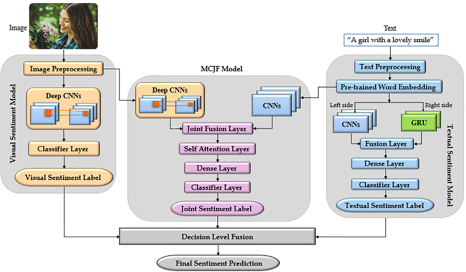
Figure 1: Multi-model fusion (MMF) model

In particular, the framework of the proposed model incorporates three deep neural networks: (1) a deep CNN is used to determine the most emotionally charged regions in an image, and (2) a BERT-based convolution-gated recurrent unit network is employed to extract the most sentimentally significant words from texts. The abovementioned methods have proven to be powerful techniques for single-model sentiment prediction. Hence, combining both approaches for feature extraction and classification yields more discriminative characteristics and, ultimately, more accurate results. A multichannel joint fusion model is proposed to exploit the intrinsic correlation between visual and textual characteristics; the basic concept for this scheme is that two distinct channels working on various modalities can extract coupling information, which is then integrated to facilitate sentiment categorization. Next, a self-attention technique is used to weigh all multimodal aspects to determine which information receives greater attention, which aids in leveraging the intricate interaction between images and texts. Lastly, a decision fusion scheme is proposed to integrate the outcomes of the individual classifiers using a rule-weighted average method that assigns different weights to each classifier’s prediction. These weights are determined through a grid search technique, optimizing the fusion of the classifiers’ results to produce the most accurate sentiment classification.

3.2 Textual Sentiment Model

A BERT-based convolution-gated recurrent unit network is proposed to extract the most important syntactic and semantic information, along with spatial, contextualized, and high-level textual information. The entire system for the textual sentiment model can be divided into the following steps: preprocessing, feature representation, and classification of input data.

Step1: Preprocessing

Different techniques are explored to preprocess the textual data: (1) lowercasing, changing all texts to lowercase. (2) removing irrelevant information, including punctuation, special characters (e.g., $, &, and %), hashtags, additional spaces, Uniform Resource Locator (URL) references, @username, stop words, and numbers. (3) Emoticon translation involves translating all emoticons into their respective terms. (4) spelling correction, correcting the word spelling to recognize the attitudes accurately. (5) language translation, converting each text to English using Google Translate [44].

Step2: Feature representation and classification

SA has recently adopted word embedding approaches, which are used to determine the linguistic relationships between words and their similarity. Word2Vec [45] and Global Vectors for word representation (Glove) [46] are two common word-embedding techniques used in earlier studies. However, they cannot distinguish between the same word in various contexts. Word embedding strategies based on transformers have been widely used to solve this issue in recent years. Related to this, BERT is currently considered the most effective vectorization model for semantic, context, location, and grammatical feature extraction from texts. Its goal is to simultaneously consider left and right contexts while pre-training deep bidirectional text representations on vast amounts of unlabeled text [47]. BERT is a multi-layer bidirectional transformer encoder based on the transformer structure [48]. It incorporates multi-head attention, which separates the model into several heads and creates various subspaces. As a result, the model can concentrate on different information aspects and fully integrate the sentence’s contextual knowledge, while parallel processing is also possible. The formula is:

Qi=𝒬Wi𝒬,Ki=KWiK,Vi=VWiV,i=1,…,12(1)

headi=Attention(𝒬i,Ki,Vi),i=1,…,12(2)

MultiHead(𝒬,K,V)=Concat(head1,…,head12)Wo(3)

where headi is the vector output by the ith head; Concat(●) specifies a splicing method that horizontally joins the matrix; Wo is a weight matrix that assigns weights to output vectors; Wi𝒬,WiK,WiV are parameter matrices projected for the Query Qi, Key Ki and Values Vi of input vectors.

The model is pre-trained with a massive unlabeled text corpus, such as Wikipedia or the Book Corpus; as a result, it can acquire a deeper and more intimate understanding of how language functions. This knowledge can be enhanced by performing the following tasks: Masked-Language Modeling (MLM) and Next-Sentence Prediction (NSP). The MLM challenge conceals a random percentage of tokens and asks users to predict their identities. Meanwhile, the objective of the NSP task is to predict if two sentences are nearby (i.e., whether one sentence follows another). In BERT design, the input Ei(i=1,2,…,t), which corresponds to the ith word in the phrase, is the sum of the word’s token embedding, position embedding, and segment embedding. BERT can be used for downstream tasks based on the pre-trained model with minimal architecture modification by jointly fine-tuning all parameters, which is comparatively affordable compared with pre-training.

In the present study, the textual sentiment model consists of multiple modules, including multichannel CNN, two layers of GRU, and a classification layer. The first part is the BERT embedding layer. After going through the necessary text processing steps for the multi-layer transformer encoder, the BERT model maps the input text words to vector representation with 768-dimensional word vectors:  BERT(T)={Ti|Ti∈Rd=768,i=1,2,…,L}.

The second part involves learning the textual features using CNN and GRU techniques. The left side uses CNN channels to extract various local properties of words between phrases. CNNs are constructed with convolutional, pooling, and fully connected layers. Let xi∈Rm represent the m-dimensional word embedding of the ith word in the phrase. Therefore, x1:n=x1⊕x2⊕…⊕xn represents a sentence of length n, where ⊕ represents the concatenation operation. In every convolution operation, a filter w ∈ Rh×m was employed on a window of h words to deliver a new feature. For instance, a feature ci is produced from a window of words xi:i+h−1 using the formula ci=f(w⋅xi:i+h−1+b), where f is a nonlinear activation function, and b is a bias term. A feature map c=[c1,c2,…,cn−h+1] was produced after applying the filter to all sliding windows of h words in the phrase. Then, the feature map c was passed into a max-pooling layer, which allowed the filter to capture the most vital information by keeping the maximum value c^=max{c} as the final feature obtained by the filter.

The procedure for a single layer has been outlined. The textual representation obtained using CNN is achieved by implementing three parallel convolution layers with window sizes of 3, 4, and 5, each equipped with 256 filters—the resulting representation, denoted as c^=[c^1,c^2,…,c^k], which can recognize diverse n-gram patterns. A batch normalization layer is added after the convolution layer to improve the network’s learning speed and provide some regularization. Finally, these features are concatenated to create a fixed-dimensional feature vector. The local features retrieved from the convolution operation are extracted from the redundant terms, and the essential features of the sentences are retained.

The right side utilizes the GRU network, which is a special type of the recurrent neural network family [49]. The internal unit of the GRU is analogous to the LSTM internal unit [50], except that the GRU integrates the forgetting port and the incoming port into a unified update port. Although it draws inspiration from the LSTM unit, it retains the LSTM immunity to the vanishing gradient problem. The simplified internal structure of GRUs allows them to train easier because less math is required to improve the internal states. The mathematical functions used to control the GRU cell’s mechanism are as follows:

zt=σ(xtWz+ht−1Uz+bz)(4)

rt=σ(xtWr+ht−1Ur+br)(5)

ℏt=tan(rt×ht−1U+xtW+b)(6)

ht=(1−zt)×ℏt+zt×ht−1(7)

where Wz,Wr,W represent the weight matrices for each connected input vector; Uz,Ur,U indicate the preceding time step’s weight matrices; and bz,br, and b are bias, whereas σ, rt, zt, ℏt denote the logistic sigmoid function, the reset gate, the update gate, and the candidate hidden layer, respectively. Two layers of the GRU network are designed to extract contextual and high-level textual information with long-term dependencies. The number of hidden layers is similar to that of CNN filters, which is 256.

Next, the right-side global feature vector fg= TextGRU is merged with the left-side local feature vector fc= TextCNN. A fused text feature vector with numerous global and local features is then produced ft= Concat(fc,fg) as a result of the second part.

The last part is sentiment classification, in which the fused text feature vector is used as input to a GlobalAveragePooling1D layer for improved representation. It uses a parser window that moves across the features and pools the data by averaging it, resulting in a one-dimensional (1D) feature vector with shape (batch size, features), followed by a dropout layer with a 50% probability to prevent overfitting and a dense layer (fully connected) with 128 units and Rectified Linear Unit (ReLU) as an activation function. Finally, the resulting textual representation Ft is passed into the SoftMax classifier, which predicts the final sentiment as follows:

p(s)=Softmax(ws,Ft)(8)

LCE=−∑log⁡(p(s),y)(9)

where, ws represents the parameters of the SoftMax layer, p(s) denotes the probability distribution of sentiment prediction, and y represents the actual sentiment class. The model is trained by lowering the Cross-Entropy (CE) loss.

3.3 Visual Sentiment Model

A deep CNN is proposed to define the most critical and emotional regions in images. The entire system for the visual sentiment model can be divided into the following steps: preprocessing, feature extraction, and classification of input data.

Step1: Preprocessing

Preprocessing is an important step that must be taken to classify the emotion of an image effectively. As a result, several preprocessing procedures are performed: (1) resizing (where all images must have the same size), the input images are resized into a [299 × 299]-pixel range for the Getty and iStock datasets and [300 × 300] for the Twitter datasets. (2) Normalization, also known as data rescaling, translates image data pixels to a predetermined range, most often (0,1) or (1,1). (3) Image enhancement improves image quality and information content.

Step2: Feature representation and classification

A CNN based on the Inception-V3 architecture is developed for the visual sentiment model. The Inception v3 architecture [51] was introduced in 2015, comprising 42 layers of symmetrical and asymmetrical building elements, such as convolutions, average pooling, max pooling, concatenations, dropouts, and fully connected layers. According to GoogLeNet [52], Inception-V3 introduced an inception model that combines convolutional filters of various sizes into a single filter. As a result of this design, fewer parameters must be trained, requiring less computation. Fig. 2 depicts the fundamental architecture of Inception-V3 [53].

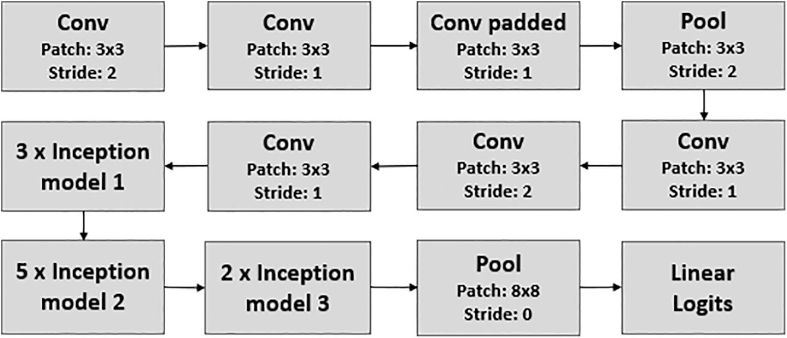
Figure 2: The inception architecture

To properly apply the Inception-V3 architecture to our work, transfer learning is used to transmit knowledge from a source area to a target area for an accurate classification model. The choice of the inception model is made to achieve a balance between feasible accuracy and performance (determined based on the number of parameters). Inception networks were created to increase the efficiency of convolutional layers by injecting sparsity into the convolutions. It can provide highly accurate results on the ImageNet dataset while utilizing fewer parameters. Thus, a new visual network can be built on the learned weights.

The visual sentiment classification model consists of two main parts: feature extraction using CNN and classification using the SoftMax layer. The pre-trained Inception v3 model is used as the base model and is fine-tuned with the sentiment image dataset. The first layers receive multiple raw images as input and output tensors with dimensions of 8 × 8 × 2048. Then, these tensors are sent to an average pooling layer with an 8 × 8 filter size to make a 1 × 1 × 2048 feature vector. The role of average pooling is considered to minimize computing complexity and data conflict. Next, a dropout layer with a 40% probability is inserted after the pooling layer to prevent overfitting, followed by a flattened layer to produce a 1D feature vector with a size of 2048. The classification layer is the final layer, in which the visual representation Fv is transmitted to the SoftMax classifier to predict the final sentiment, as seen in Eqs. (8) and (9), by replacing the textual representation Ft with the visual representation Fv.

3.4 Multimodal Fusion Methods

3.4.1 Multichannel Joint Fusion Model via Intermediate Fusion

Various data modalities typically contain supplementary information. As shown in Fig. 1, the word “lovely” represents text-specific information that is difficult to discern from the image. In contrast, “smiling face” and “flower” represent image-specific data that cannot be captured by textual tags. The two types of characteristics are complementary to the analysis of emotions. Thus, this study uses the MCJF model to combine visual and textual features for MSA. In this manner, the inherent correlation between both modalities can be captured.

This scheme uses two unique channels at the input layer to handle multichannel data independently. A deep visual feature vector is first extracted using the pre-trained Inception-V3 model with a size of 1 × 1 × 2048 from the image part. Then, a high-level textual feature vector is extracted from the text part using the pre-trained Bert-based multichannel CNN with a size of 38 × 256. Finally, the two feature vectors are fed to the fusion layer, which expects the two vectors (i.e., the image feature vector Vi and the text feature vector Vt) to have the same dimension. As the image vector has a higher dimension than the text feature vector, we must map its features onto the textual feature space. This process is accomplished by adding a reshaped layer to obtain the two-dimensional (2D) image feature vector. Then, a dense linear layer with 128 neurons embeds the image and text features into an S-dimensional common space. This layer is defined as follows:

Vi′=Relu(WiVi+bi)(10)

Vt′=Relu(WtVt+bt)(11)

where (Vi′,Vt′) represents the new image and text feature vectors, which have the same dimension. (Wi,Wt) represents the weights, and (bi,bt) is the bias. To produce the fused feature vector Jf, an average fusion rule is employed to combine the two feature vectors (Vi′, Vt′) as follows:

Jf=Average(Vi′;Vt′)(12)

The fundamental principle is that two distinct channels operating on different modalities can extract coupling information. Then, this information is combined to enhance SA and exploit the inherent connection between texts and images. Our approach relies on the idea that the visual information and certain key emotional words in the input sequence are essential in determining the actual sentiment. Therefore, to define the contribution of each modality to the sentiment polarity of a given image-text pair, a self-attention mechanism is used to highlight the sentimentally rich information associated with the multimodal feature vector for accurate SA [54]. In particular, the network automatically calculates the important weights for each modality based on the multimodal feature vector, as shown below:

ef=φ(w∗Jf+b)(13)

vf=exp(ef)∑fexp(ef)(14)

where ef is the un-normalized attention score indicating how accurately the vector Jf reflects the sentiment, vf is utilized to normalize the attention over the sequence using the SoftMax function; w and b represent the learnable weights, whereas φ is the nonlinear activation function (e.g., tanh). As a result, distinct input modalities in a self-attention network can interact with one another (“self”) to determine which input receives greater attention, highlighting the importance of the sequence’s multimodal input elements. The joint attended multimodal features are formed by computing the weighted average throughout the entire feature sequence, as shown below.

m=∑fvf,Jf(15)

The produced multimodal features m are then used as input for the remaining part of the model, consisting of two dense layers with 256 and 128 units, and ReLU as an activation function. A dropout layer with a 20% probability is used to prevent overfitting. The final representation M is fed into the SoftMax classifier to predict the final sentiment as follows:

p(s)=softmax(ws,M)(16)

LCE=−∑log⁡(p(s),y)(17)

where, ws denotes the SoftMax layer parameters, p(s) is the sentiment prediction probability distribution, and y is the actual sentiment label of the training data. The model is trained by lowering the CE loss for optimal performance.

3.4.2 Decision Fusion via Rule Weighted Average Method

The sentiment from the three modalities—the Visual Sentiment Model (VSM), the Textual Sentiment Model (TSM), and the MCJF Model—is first classified before attempting to combine the outcomes. The predicted probabilities of the sentiment classes from the three modalities are then evaluated. In late fusion, the individual predictions are combined using the rule weighted average method, in which the contribution of each model is weighted proportionally to its capability or skill. The weights are small positive values between 0 and 1, and the sum of all weights equals 1. For example, suppose we have three prediction lists, pv, pt, and pm, which represent the predictions generated by the VSM, TSM, and MCJF, with pv=[pv1,pv2,pv3], pt=[pt1,pt2,pt3],pm=[pm1,pm2,pm3], each containing the probability distribution for a specific class label predicted by each classifier. Therefore, the rule weighted average method can be calculated by taking the sum of the product of the predicted probabilities from the sentiment labels into weight and dividing it by the sum of weights, which can be written as:

Weighted Average=(pv∗W1+pt∗W2+pm∗W3)/(W1+W2+W3)(18)

Here, W1, W2, and W3 represent the weights corresponding to the relative importance of each modality to the final prediction. Given that the total sum of all weights is 1, this indicates that the predicted probabilities from the sentiment labels generated by each modality are multiplied by its corresponding weight. The final prediction can then be determined by calculating the “argmax” of the summed probabilities for each class label, which returns the class index with the highest probability value.

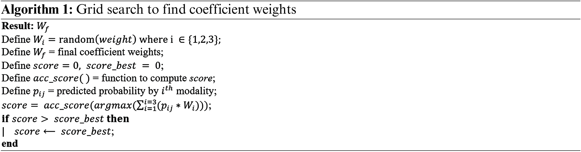
The grid search algorithm is used to compute the weight of each model, which represents the most comprehensive approach for estimating weights because it uses a unit norm weight constraint to ensure that the vector of weights sums to one. The grid search works by defining a grid of parameters—in our case, weights for each modality—and then evaluating model performance for each point in the grid. We use a predefined performance metric (i.e., accuracy) to measure how well the model performs with each combination of weights. Grid search aims to find the optimal weights that maximize the model’s performance on the validation set. This process entails the following steps:

1) Initially, a course grid of weight values from 0.1 to 0.9 is established as weight = [0.1, 0.2, 0.3, 0.4, 0.5, 0.6, 0.7, 0.8, 0.9], and all possible combinations are generated using the Cartesian product. One disadvantage of this strategy is that the weight vectors will not sum to one (the unit norm), as required. As a result, each generated weight vector is forced to have a unit norm by computing the sum of the absolute weight values (referred to as the L1 norm) and dividing each weight by that value. Then, the weight vectors produced by the Cartesian product can be systematically listed, normalized, and predicted to determine the best weight for use in our ultimate weight-averaging process.

2) For each sentiment class, the weighted average is calculated using the predicted probabilities of the sentiment labels and the coefficient weights created in the previous step.

Pj=∑i=1i=3(pij∗Wf)(19)

where, i represents the modalities (visual, textual, intermediate fusion), j represents the sentiment labels, Wf denotes the final coefficient weights, pij defines the predicted probability for the ith modality, and Pj is the final probability for the jth class.

3) The final predicted label y^ is calculated by locating the class index, which corresponds to the highest probability value, as shown below:

y^=argmax(Pj)(20)

The proposed framework can analyze the problem in which a training instance can be an image-text pair, an unpaired image, or unpaired text. When an image-text pair is obtained, the three classifiers (i.e., VSM, TSM, and MCJF) are trained, and the rule-weighted average method is then applied to reach the final classification. The visual classifier makes the final prediction when the instance is an unpaired image. Similarly, when the instance is an unpaired text, the textual classifier makes the final prediction. The observed experimental coefficient weights are w = [0.143, 0.423, 0.423], w = [0.143, 0.357, 0.5], w = [0.333, 0.222, 0.444], and w = [0.421, 0.316, 0.263] for the BG, BIS, Twitter, and MVSA-Single datasets, respectively.

3.5 The Visual-Textual Explainable Model

Deep neural networks can distinguish human emotions, and most of the related literature has focused on new designs to improve this task, with few attempts to explain these models’ decisions. Users may be unable to check the results of “black box” models because their core logic is hidden. Consequently, these models must meet the justifiability, usability, and dependability requirements for an SA system to be accepted. LIME aims to define an explainable model over an interpretable representation that is locally accurate for any classifier’s predictions. After dividing the input into features, it randomly perturbs each feature S times and analyzes the model’s output logits for class c. LIME then produces a linear model that maps each feature’s perturbations to their logits of c. The linear model’s weights explain each feature: a positive weight supports class c, while a negative weight opposes it. Furthermore, the higher the absolute value of the weight, the more significant its contribution.

Weights can also produce an understandable representation. Each feature is usually a segment for images, so the sections with the most significant absolute weights can be highlighted in different colors to depict negative and positive effects. Text characteristics are usually presented as words, so a histogram of word weights can explain them. Mathematically, LIME provides a solution to the following optimization problem:

ξ(x)=argming∈G ℒ(f,g,∏x)+Ω(g)(21)

An explanation model can be described as a model g∈G, where G is the family of explanation models (i.e., linear models), in which Ω(g) be a metric for explaining g∈G complexity (as opposed to its interpretability). In addition, f represents the explained model, where f(x) is the likelihood that x belongs to a particular class. To determine the locality around x, the ∏x(z) is utilized as a closeness measure between an instance of z and x. Meanwhile, the loss ℒ(f,g,∏x) represents the degree to which g approximates f faithfully in the locality given by the weighting kernel ∏x, which is usually an exponential kernel of a distance function, in this case, the Euclidean distance. Eventually, the loss ℒ(f,g,∏x) is reduced while having Ω(g) be low enough to be understood by humans to assure both interpretability and local fidelity.

To explain the model results, we have enhanced the fundamental LIME method to make it applicable to our proposed MMF model by using LIME Explainer for textual and visual content. In the case of image data, the explanations are made by generating a new dataset of perturbations surrounding the instance that needs to be explained. For this purpose, we use a simple linear iterative clustering (SLIC) segmentation algorithm [55] that groups pixels in the unified 5-dimensional color and picture plane space to effectively construct condensed, relatively uniform superpixels. The generated model is then used to forecast the class of the recently created images. Each perturbation’s importance (weight) in predicting the related class is determined using cosine similarity and weighted linear regression. Ultimately, LIME explains the image regions (superpixels) and the most important words that considerably influence the image–text instance’s assignment to a specific class.

Fig. 3 displays some of the explanations provided by LIME for the BG dataset; as can be seen, the explanation model has effectively highlighted the most critical terms in the text section, which contribute more to the final correct prediction and have greater weight. Similarly, the image part provided the following explanations: Image (a) represents the original image, while image (b) displays the superpixels where negative and positive contributions are considered (pros in green, cons in red).

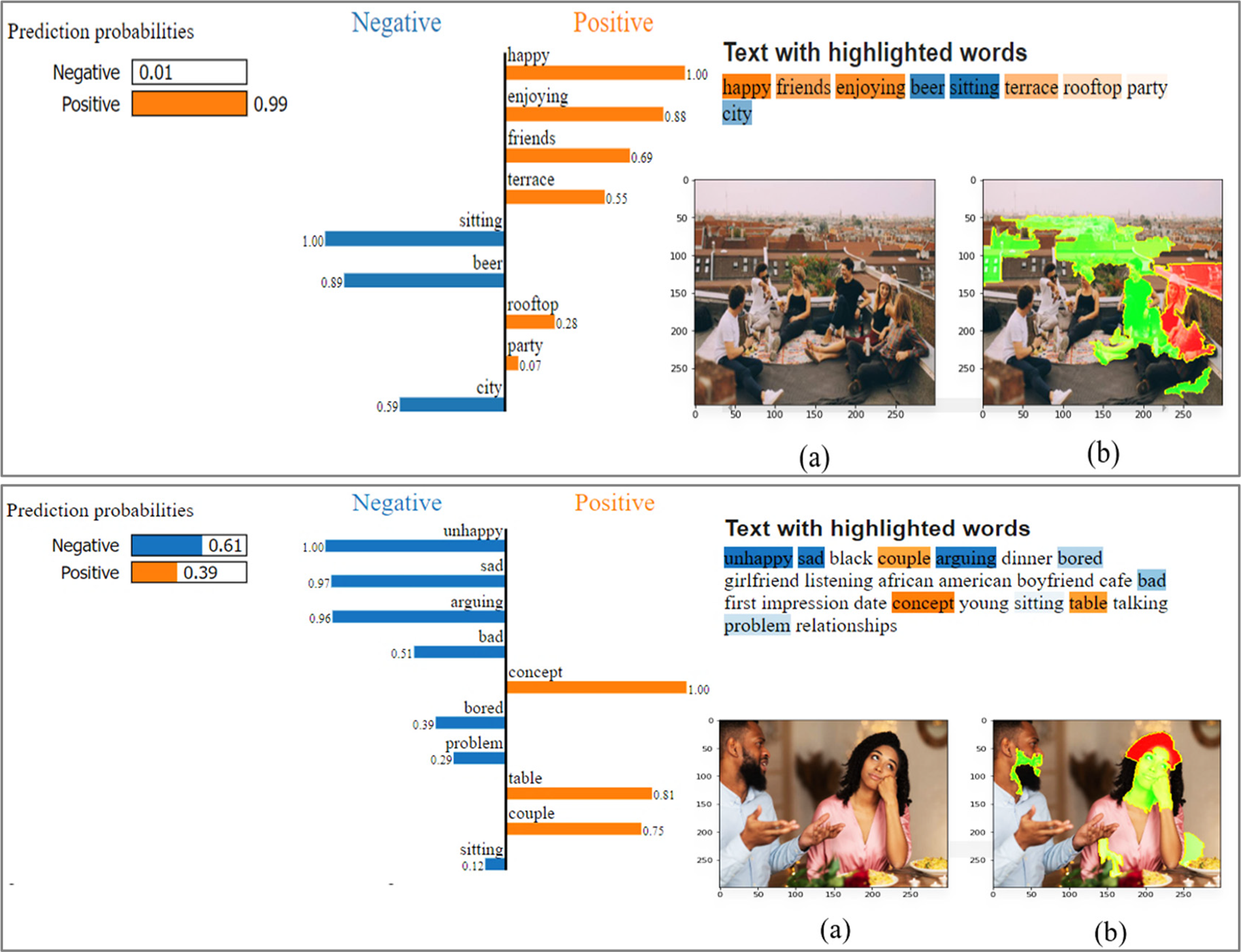
Figure 3: The model explanation for the BG dataset

4  Experimental Setup

4.1 Datasets

Four social media datasets are used to evaluate the efficacy of the proposed MMF model. The datasets are discussed in detail as follows:

1) Getty Images: Getty Images [56] provides creative photographs, videos, and audio to businesses and consumers, with over 477 million resources in its collection. The main advantages of Getty Images are its user-friendly, efficient query-based search engine and its formal yet descriptive image descriptions. In particular, 3244 Adjective-Noun Pairs (ANPs) from the Visual Sentiment Ontology [57] are used as keywords to collect 20,127 image-text samples, with 10098 and 10029 for the positive and negative classes, respectively. The dataset is named “Binary_Getty” (BG), which includes images, relevant textual explanations, and labels.

The initial labeling was accomplished using the sentiment scores associated with ANP keywords. To achieve strong labeling, we further employed the Valence-Aware Dictionary and sentiment Reasoner (VADER) [58], a lexicon, and a rule-based SA tool [59] to label the preprocessed textual description. Then, we selected only the text samples for which the ANP and VADER sentiment scores were the same. Due to the close relationship between the text and image content of Getty Images, we classified the image samples based on the accompanying textual labeling. Finally, three volunteers were chosen to assess the quality of our datasets. Each image-text sample was graded 1 (suitable) or 0 (unsuitable). The results showed that 95% of the samples were suitable and 5% were unsuitable; we only considered the samples with grade 1 (suitable) and ignored the others.

2) iStock Images: iStock Images [60] provides international, royalty-free microstock photos online, particularly images, graphics, clipart, videos, and audio tracks. In exchange for royalties, artists, designers, and photographers worldwide offer their work to iStock. The same procedure from Getty Images was implemented; 3244 ANPs were used as keywords to retrieve 19,279 image-text samples, with 10587 and 8692 for positive and negative classes, respectively. The dataset, named “Binary_iStock” (BIS), comprises images, labels, and relevant textual descriptions. We used the same labeling procedure demonstrated for the Getty Images dataset to establish the final labeling of the iStock Images dataset.

3) Twitter Dataset: Additionally, we gathered a new dataset from Twitter. English tweets with text and photos are specifically gathered using the Twitter streaming Application Programming Interface (API) [61], with user-generated hashtags as keywords. We carefully filtered out duplicated, low-quality, pornographic photos and all text that was too short (less than five words) or too long (more than 100 words). We used VADER, a lexicon, and a rule-based SA tool to speed up the labeling process and predict text sentiment polarity. Then, a visual sentiment analysis model [62] based on the Twitter for SA (T4SA) [63] dataset is used to predict the polarity of the visual sentiment. Based on the projected sentiment polarity and visual-textual content, the tweets were manually categorized into positive, negative, and neutral sentiment polarities. Finally, we obtained 17,073 high-quality tweets containing image-text pairs with 6075, 5228, and 5770 for positive, negative, and neutral classes.

4) Multi-View Sentiment Analysis (MVSA): The MVSA-Single dataset [64] comprises 5129 image-text pairs extracted from Twitter. After presenting each pair to a single annotator, the annotator assigned the image-text pair one of three polarities (neutral, negative, or positive). Like [65], we first delete tweets with contradicting textual and visual labels. In cases where one modality is labeled neutral while the other is labeled positive or negative, the ultimate polarity assigned to multimodal data is positive or negative. Thus, we obtain a new MVSA-Single dataset containing 4511 text-image pairs with 2683, 1358, and 470 for the positive, negative, and neutral classes.

4.2 Implementation Details

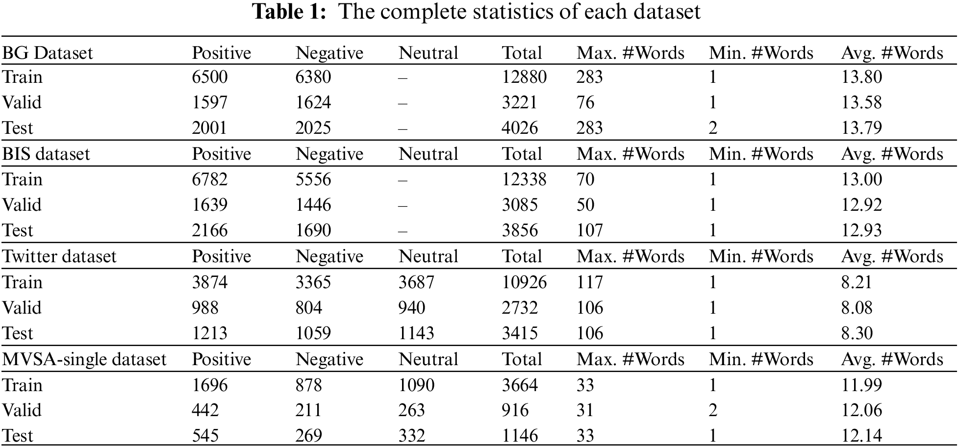
The datasets were divided into training, validation, and testing sets, with the proportions being 60:20:20. Table 1 shows the complete statistical information for each dataset. It can be observed that the MVSA-Single dataset is significantly unbalanced and has various data distributions. The absence of sampling may pose challenges to effectively studying the smaller dataset category during training. This results in classifying all data into the same class, thereby leading to classifier failure. Thus, a random up-sampling technique was employed on the smallest category within the MVSA-Single dataset to minimize the effects of data imbalance during the experiment. In the experiments related to binary class datasets, the final classifier layer was configured with one unit and a sigmoid as the activation function. We used a batch size of 32 and Adam with a learning rate of 0.001 as an optimizer to train the textual and visual models. The intermediate fusion model, on the other hand, is trained using the Stochastic Gradient Descent (SGD) optimizer with a learning rate of 0.0001. To ensure a safe upper bound, the proposed models were trained for 100 epochs with early stopping using a patience value of 3. The model was evaluated using accuracy metrics and a loss function based on cross-entropy. The research used an NVIDIA Tesla K80 Graphics Processing Unit (GPU) and 16 GB of Random-Access Memory (RAM) to conduct the experiments. All codes were written in Python 3.7.13 using the Keras library in the Google Colaboratory environment.

4.3 Results and Analysis

The following evaluation metrics were employed to evaluate the proposed model’s efficacy and conduct a comparative analysis with previous research: precision, recall, F1-score, and accuracy. These measurements were explained and computed as follows:

Accuracy is the proportion of accurate projections to the total number of examined instances, which indicates the model’s overall performance.

Accuracy=TP+TNTP+TN+FP+FN(22)

Precision is the proportion of accurate positive results to the total number of positive outcomes anticipated by the classifier. It evaluates the model’s ability to identify only the relevant instances accurately.

Precision =TPTP+FP(23)

Recall, also called sensitivity, is the proportion of accurate positive outcomes to the total number of actual positive outcomes (the sum of true positives and false negatives). It quantifies the model’s capacity to recognize all relevant instances.

Recall =TPTP+FN(24)

F1-score is the harmonic mean of precision and recall. It aims to balance these two metrics and provides a single score that reflects the model’s overall performance. This measurement has a value between 0 and 1, and if the classifier correctly classifies all samples, it returns a value of 1, indicating a high degree of classification success.

F1−score =2×precision×recallprecision+recall(25)

TP = true positive, TN = true negative, FP = false positive, and FN = false negative. All evaluation measures range from 0% to 100%, with higher values indicating excellent model performance. These metrics offer a comprehensive understanding of the model’s performance. Table 2 demonstrates the results of the model variants compared to the MMF model, which indicates the following observations.

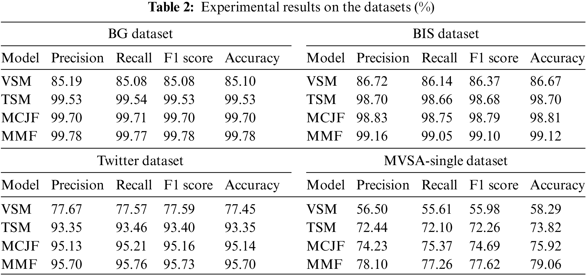
Firstly, the VSM demonstrates the poorest performance. The primary reason is that images lack the contextual information needed for a more precise interpretation. Unlike words, visuals cannot directly describe emotions. Thus, adding additional modality information, such as textual data, improves sentiment performance.

Secondly, the performance of the TSM surpasses that of the image-based analysis model. This can be attributed to the superior efficacy and informational value of emotional cues in textual content compared to visual data. We credit the BERT models’ success to their ability to learn from large datasets, enhancing their effectiveness in extracting task-relevant features.

Thirdly, it has been observed that the multimodal approach (i.e., MCJF) exhibits superior performance compared to its related unimodal baseline methods by a significant margin. This illustrates that depending exclusively on textual or visual elements is generally inadequate for sentiment analysis. Indeed, a more comprehensive set of information can be derived by utilizing various modalities, which synergistically aid in capturing the semantic characteristics and the natural relationship through integration among diverse data modalities. Finally, by combining the confidence scores of the three separate models, MMF can improve performance even in the absence of one modality, resulting in more accurate decision-making.

As previously stated, the results demonstrate that TSM outperforms VSM according to the evaluation criteria across all datasets. Specifically, the BG and BIS datasets achieve significantly higher accuracy rates (99.53% and 98.70%) than the Twitter-based datasets, which achieved accuracy rates of 93.35% and 73.82%, respectively. Furthermore, comparable results were obtained for the VSM approach, which achieved an accuracy of 85.10% and 86.67% for the BG and BIS datasets, respectively, while achieving an accuracy of 77.45% and 58.29% for the Twitter and MVSA-Single datasets. As a result, the proposed model’s final sentiment was significantly influenced, resulting in accuracy rates of 95.70% and 79.06% for the Twitter and MVSA-Single datasets, respectively. In comparison, the BG and BIS datasets achieved higher accuracy rates of 99.78% and 99.12%, respectively.

The performance of the proposed models on the Twitter and MVSA-Single datasets is less impressive than on the Getty and iStock datasets for several reasons, including the fact that most of the tweets are short, informal, and unrelated to the image content. In addition, low-quality photos are frequently included in tweets, which can reduce the model's effectiveness. Despite being a benchmark dataset, the MVSA-Single dataset poses various challenges: 1) the texts contain much noise, which demands extensive preprocessing and spelling correction, as illustrated in Section 3.2; and 2) the distribution of the classes is significantly unbalanced; thus, a random up-sampling technique was employed to achieve a better and more balanced distribution for each class. However, the proposed MCJF still exhibits a significant advancement over earlier models. Meanwhile, weighted late fusion is more effective than independent models in categorizing emotion.

The F1-score for each model’s polarity and a comparison of the proposed model research findings across all datasets are shown in Figs. 4 and 5, respectively. As can be seen, the BG and Twitter datasets have a higher F1-score for the negative class across all the classifiers, achieving the highest value on late fusion with 99.78% and 97.33%, respectively. In contrast, the BIS and MVSA-Single datasets have a higher F1-score for the positive class across all the classifiers, achieving the highest value on late fusion with 99.22% and 83.72%, respectively. Thus, the proposed model effectively utilizes the correlation between visual and textual modalities across all datasets.

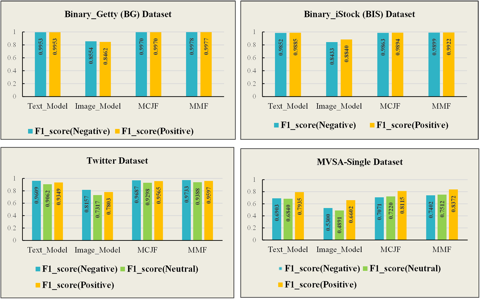
Figure 4: F1-score for each model’s polarity

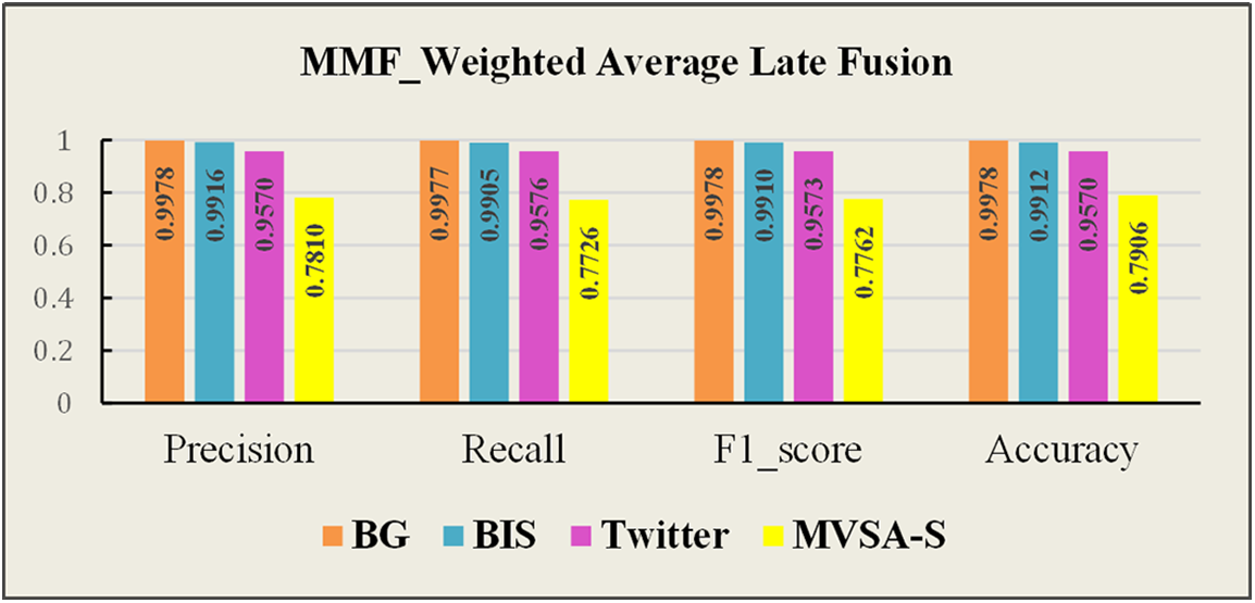
Figure 5: A comparison results of the proposed model

Meanwhile, a comparison between the confusion matrix of the MMF model on the datasets is shown in Fig. 6. It can be observed that the proposed model on the BG dataset fared better at correctly classifying the negative polarity. In contrast, the proposed model on the BIS dataset performed better in correctly classifying the positive polarity while achieving reasonable accuracy in detecting the negative polarity. Similarly, the proposed model in the Twitter and MVSA-Single datasets fared better in correctly classifying the negative and positive polarities while achieving reasonable accuracy in detecting the neutral polarity. The proposed model can correctly classify 98% and 95% of negative and positive classes from the Twitter dataset while correctly classifying 85% and 73% of positive and negative classes from the MVSA-Single dataset.

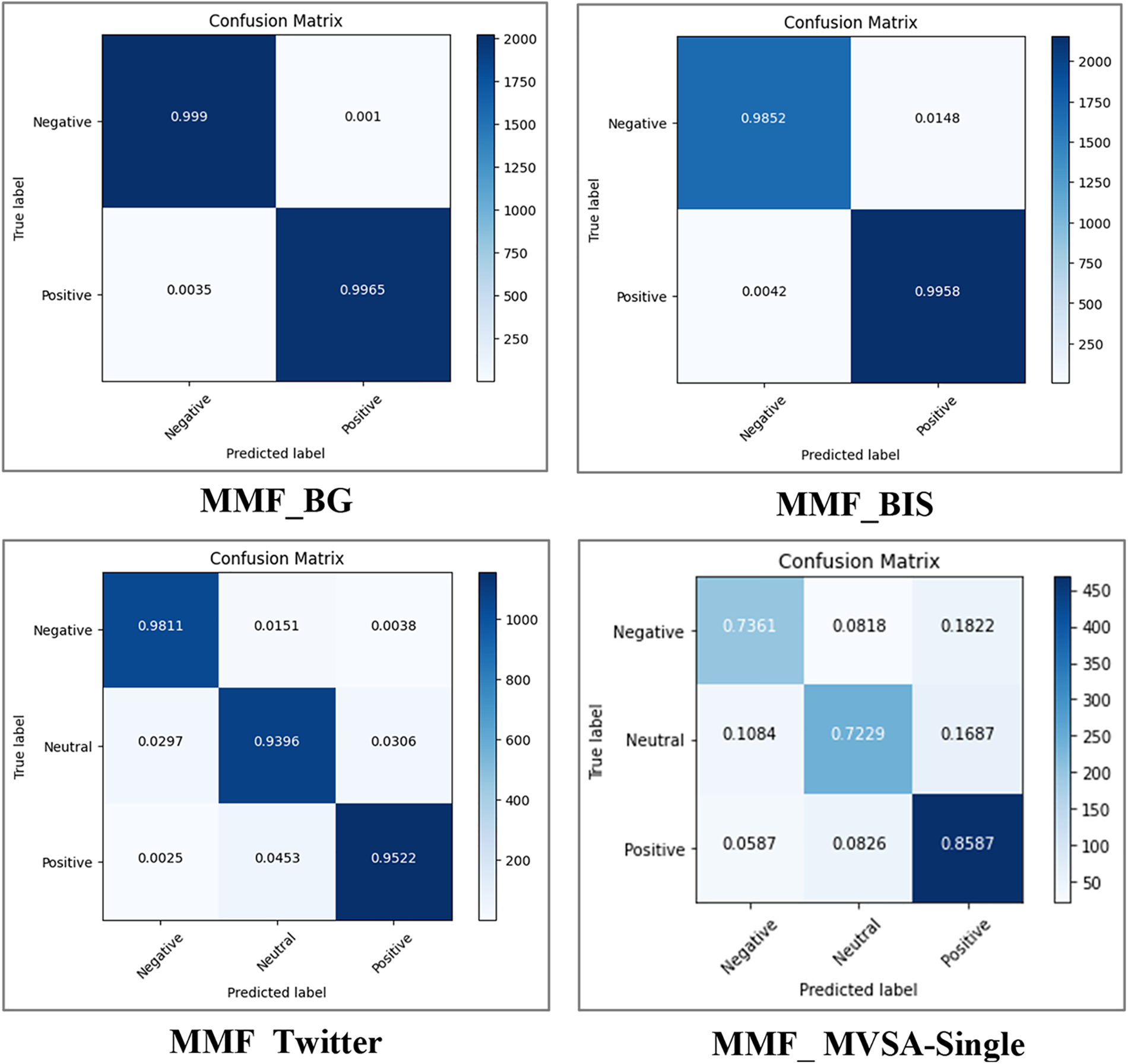
Figure 6: A comparison between the confusion matrix of the MMF model

A comparison of the training duration between the proposed models is further shown in Table 3 to provide more experimental details. As can be seen, the MCJF model required more training time, which is reasonable given the time required to extract and combine the coupling features from the two modalities. In contrast, the TSM has taken less training time across all the datasets. Compared to TSM, VSM has taken more time, and this is because image data is more complex than text data. Also, the dataset’s size significantly impacts the training duration; the MVSA-Single dataset has taken less time for training, while the BG dataset considerably takes more time for training, especially for the MCJF model. As for the late fusion model, which does not require training where the predictions from each model must be combined using the weighted average method, the training time has been considerably less than for the other models and has been almost entirely consumed by the grid search algorithm that is used to estimate the optimal list of weight values required by each classifier.

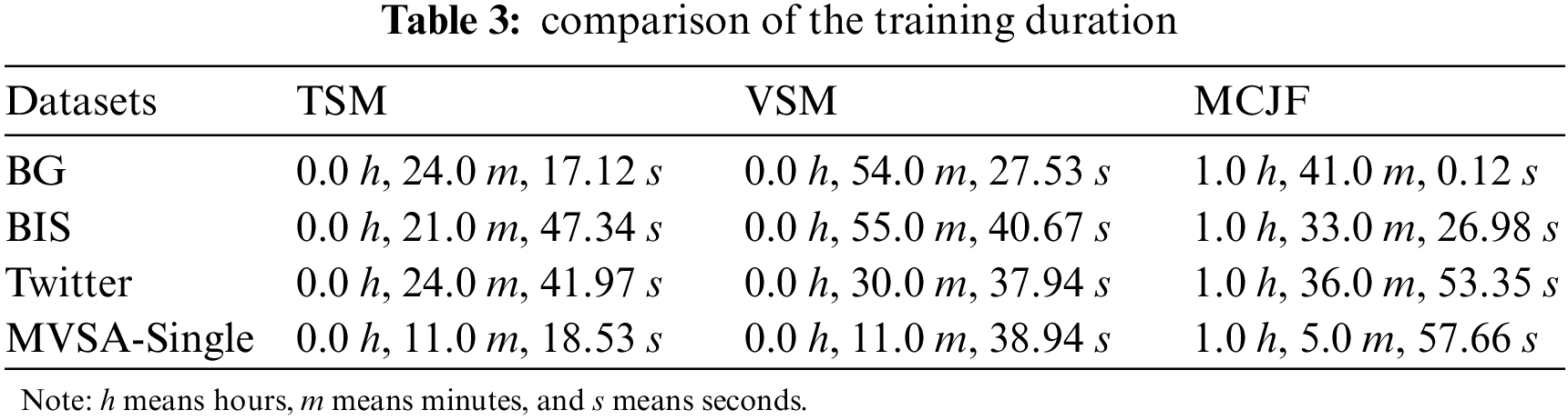
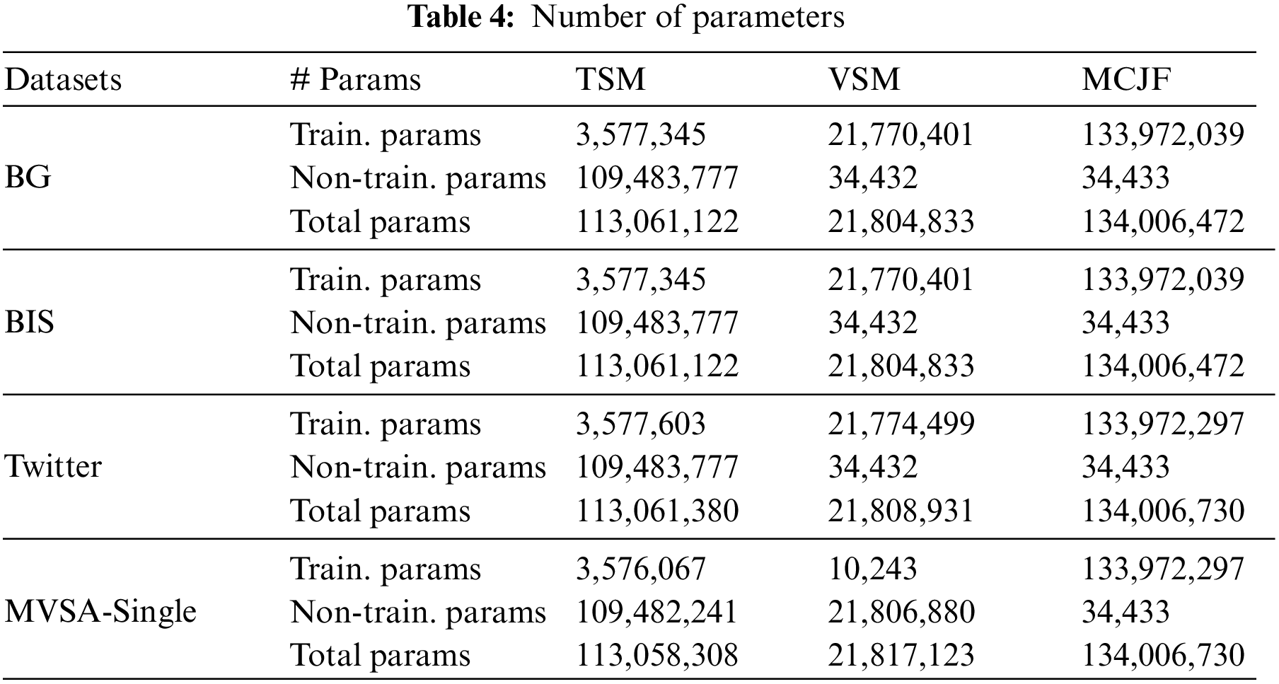
Table 4 illustrates the number of parameters consumed by each proposed model across the datasets. Our proposed MMF’s complexity can be comprehended in various ways. The model includes two neural networks for image and text processing and classification, as well as an MCJF model that incorporates the coupling features. Finally, decision fusion combines all of the predictions from each model. This may indicate greater complexity in terms of parameters and architecture when compared to single-modality models. The model’s learning mechanism is complicated, as evidenced by the learning rates and optimizer used for training. However, this additional complexity enables the model to effectively capture the intricate relationship between the visual and textual modalities, resulting in improved precision, recall, F1-score, and accuracy across all datasets.

4.4 Compared Methods and Baselines

We compared our results to the unimodal and multimodal sentiment baseline models and other recent studies on visual-textual SA.

Unimodal Sentiment Baselines: For textual modality, Single Textual Model [21], Logistic Regression (LR)-BERT, and SVM-BERT apply LR and SVM to predict sentiment based on textual features retrieved using BERT and CNN, GRU [49], and CNN [66]. For visual modality, Single Visual Model [21], SVM: an SVM classifier estimates sentiment based on visual features extracted with a pre-trained Inception-V3 model, VGG16 [67], and ResNet50 [68].

Multimodal Sentiment Baselines: Different approaches have been proposed; Early Fusion-1 [21], Early Fusion-2: an SVM classifier predicts sentiment based on the concatenation of visual and textual features extracted by Inception-V3 and paragraph vector, and Early Fusion-3: an LR classifier predicts sentiment by combining visual and textual features extracted using Inception-V3 and BERT with CNN. Late Fusion-1 [21], Late Fusion-2: an average sentiment score is applied on single visual and textual models, with both models classified using SVM, where the visual and textual features are extracted using Inception-V3 and paragraph vector, and Late Fusion-3: a classification-based approach using SVM on a single visual and textual model, with both models classified using LR, where the visual and textual features are extracted using Inception-V3 and BERT with CNN.

Comparison to Current Visual-Textual SA Research: Our results were compared to other recent studies on visual-textual SA. The comparison is unfair because other articles used different datasets, especially the BG and Twitter datasets. Still, it sheds light on the factors that went into it and the categorization strategy employed with their results. The comparative findings are shown in Tables 5–8, which are discussed in Section 5. To our knowledge, a model that uses the BIS dataset obtained from the iStock website has yet to be published. As a result, the proposed models were compared only with the previously described baseline models.

5  Discussion

5.1 Comparative Results on the BG and BIS Datasets

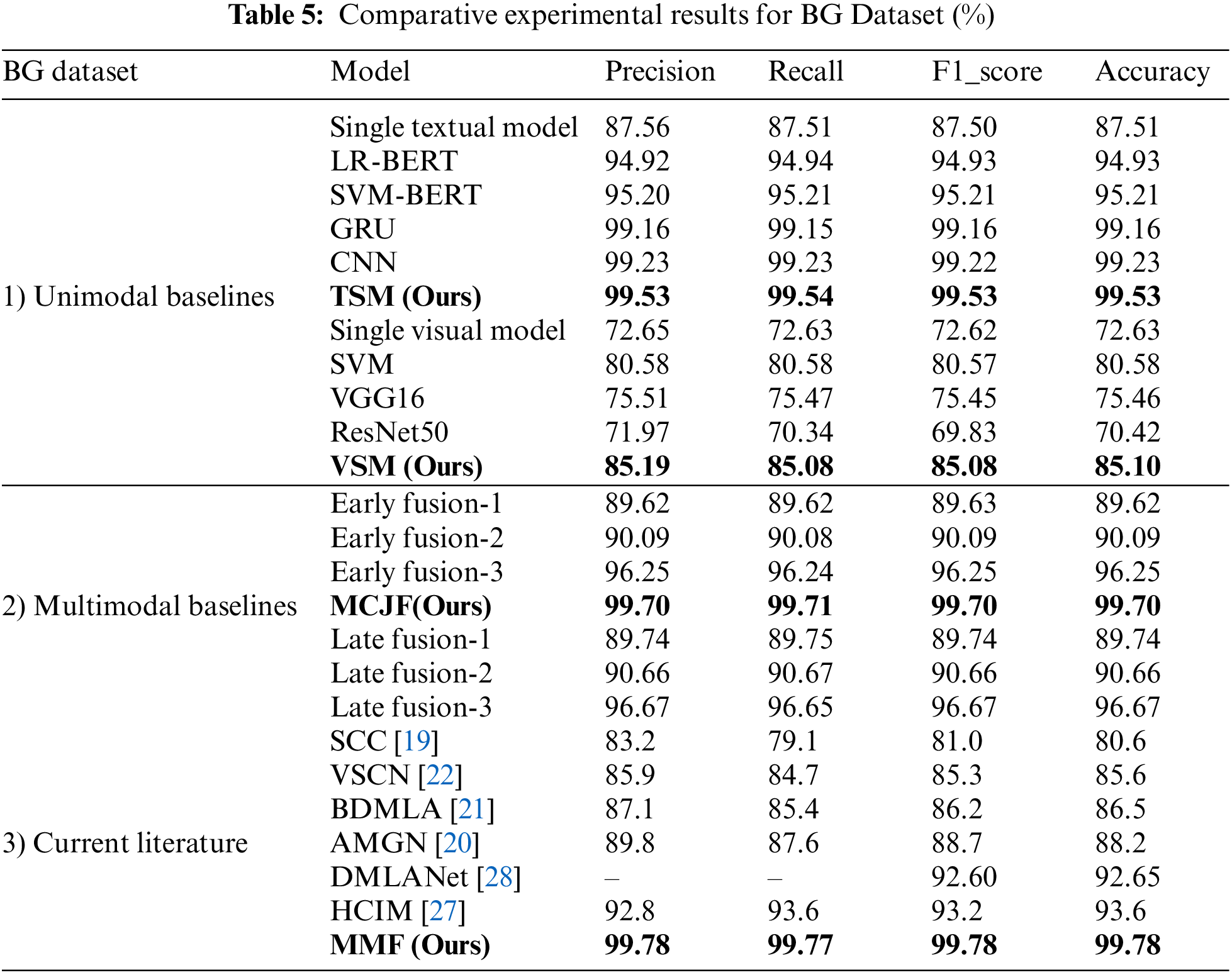
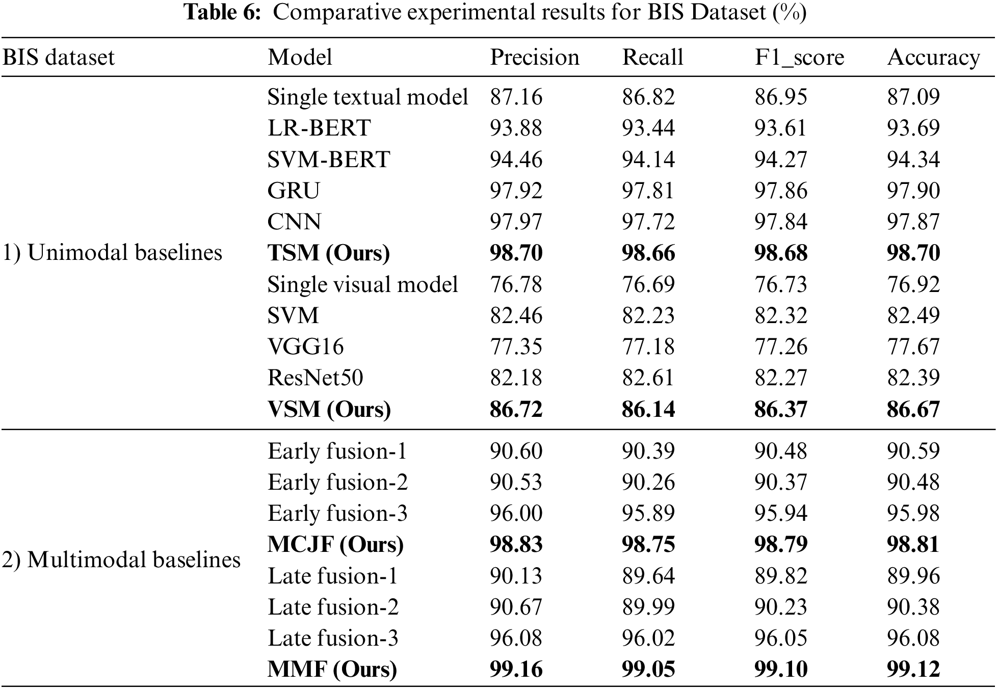
Tables 5 and 6 provide the comparative results for the BG and BIS datasets. As can be seen, the proposed VSM and TSM outperform the unimodal visual and textual baselines because the VSM can pay more attention to the most effective image regions. In contrast, TSM can efficiently concentrate on the most sentimental textual words. With deep intermediate fusion, the MCJF model considerably outperforms the multimodal baselines, indicating that the MCJF model contributes much to capturing fine-grained characteristics that improve sentiment categorization. Consequently, MMF obtains better F1 and accuracy scores than other models.

A comparison of our study with the recent literature utilizing the BG dataset is further carried out to demonstrate the efficacy of our proposed approach. The comparative results reported in Table 5 indicate that the DMLANet model outperformed AMGN in terms of F1-score (92.60%) and accuracy (92.65%). In comparison, AMGN achieved an F1-score of 88.7% and an accuracy of 88.2%, which shows better performance than BDMLA and VSCN, which had 86.5% and 85.6% accuracy, respectively. The SCC model exhibited the weakest performance among all the models, with an F1-score of 81.0% and an accuracy of 80.6%. Despite HCIM exhibiting superior performance compared to other techniques, achieving an F1-score of 93.2% and an accuracy rate of 93.6%, it remains inferior to our model. The results showed that our model could compete with recent studies by achieving the highest accuracy and an F1-score of 99.78%. This demonstrates the superior performance of the MCJF in comparison to other models, as the multichannel inputs are simultaneously learned under a single learning structure, and the parameters of numerous channels can be collaboratively tuned during training. The MMF further improves performance by merging the confidence scores of three independent models.

5.2 Comparative Results on Twitter and MVSA-Single Datasets

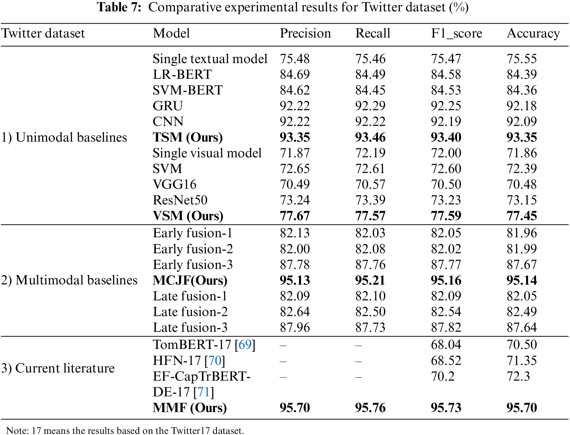
Table 7 compares the outcomes of the various Twitter dataset-based methodologies. As can be seen, the proposed TSM and VSM models outperform all the unimodal baselines, while our multimodal approaches show excellent performance over the unimodal and multimodal baseline methods. Our study is further compared with the existing literature to show the effectiveness of our proposed approach. Yu et al. [69] presented a Target-Oriented Multimodal BERT (TomBERT) model, where the target-sensitive textual representations were initially obtained using BERT. Then, a target attention mechanism was designed to generate target-sensitive visual representations. Although a series of self-attention layers were built on top to record the multimodal interactions, they neglected textual information’s impact on the picture. Zhang et al. [70] developed a Hybrid Fusion Network (HFN) to collect intra- and intermodal characteristics. They used visual characteristics to derive emotional data from written content via multi-head visual attention. Several base classifiers were then taught to acquire discriminative data from various modal representations. The main drawback of this approach is that choice diversity and classification accuracy clash as the model approaches convergence. Meanwhile, Khan et al. [71] developed a two-stream model named EF-CapTrBERT-DE, which used an object-aware transformer to translate images and non-auto-regressive text synthesis. An auxiliary sentence for a language model was then made using the translation. However, the significant variance in the utility of the visual modality and the complexity of the scene are significant limitations that restrict the efficacy of this approach.

According to the comparison results in the third group of Table 7, it can be concluded that EF-CapTrBERT-DE performed better than HFN, with an F1-score of 70.2% and an accuracy of 72.2%. Compared to the TomBERT model, which had the lowest performance with an F1-score of 68.04% and an accuracy of 70.50%, HFN exhibits a 0.48 and 0.85 improvement in F1-score and accuracy, respectively. Our proposed model outperforms the state-of-the-art by a wide margin, both in terms of F1-score (95.73%) and accuracy (95.70%), proving the efficacy of the MMF model for precise sentiment classification.

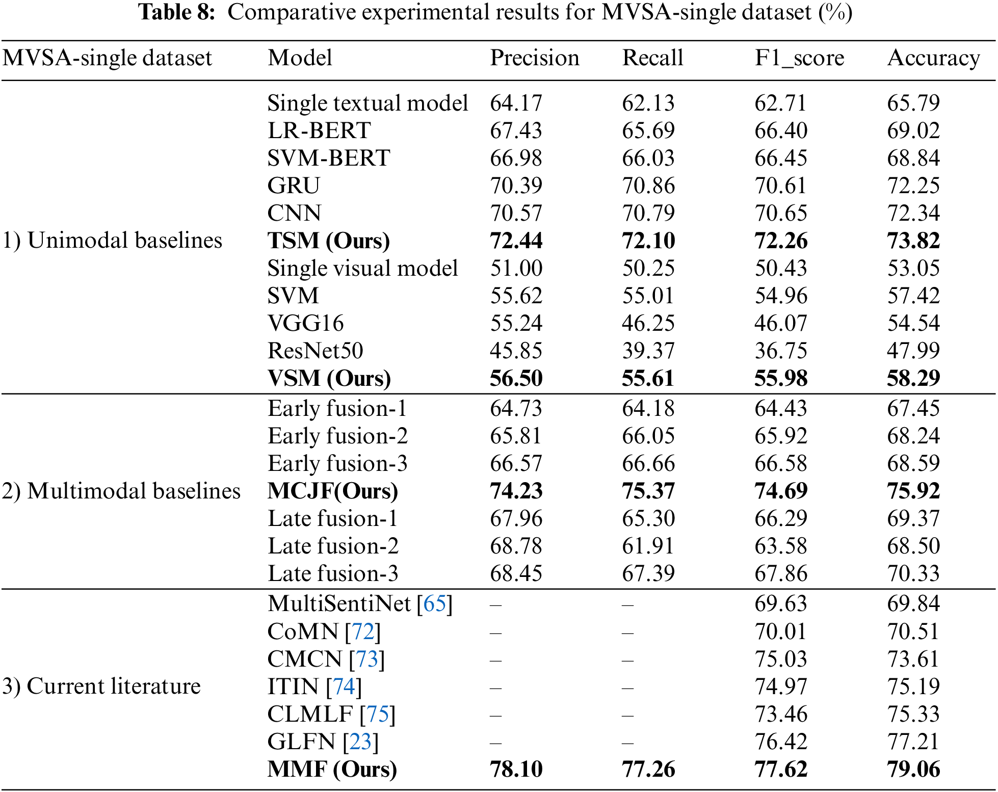
The comparative results of the different methods using the MVSA-Single dataset demonstrate the proposed models’ excellent performance compared to the unimodal and multimodal methods, as shown in Table 8. To further assess the efficiency of the proposed model, we compare our findings to the current literature. Xu et al. [65] introduced MultiSentiNet, a deep semantic network that uses an attention-guided visual feature LSTM model to extract emotional terms from tweets and integrate them with visual features to model picture-text content associations. However, it emphasized the visual elements more than the impact of the text on the image. A stacked Co-Memory Network (CoMN) was developed by Xu et al. [72], which employs an iterative approach that leverages textual data to identify significant visual features while utilizing image data to pinpoint relevant textual keywords. However, coarse-grained attention may cause data redundancy and must be improved. Peng et al. [73] developed a framework for a Cross-Modal Complementary Network (CMCN) with hierarchical fusion that may fully incorporate multiple modal features while lowering the danger of merging irrelevant modal information. Zhu et al. [74] used an Image–Text Interaction Network (ITIN) to study the emotional visual areas and written information in multimodal SA. First, the region word correspondence was extracted using a cross-modal alignment module, after which multimodal characteristics were integrated using an adaptive cross-modal gating module. The model’s weakness is that fine-level interaction would be ineffective if the associated text did not specify emotional image areas. According to this scenario, prediction accuracy would be assessed using unique modal and contextual representations. Meanwhile, Contrastive Learning and Multi-Layer Fusion (CLMLF) was proposed by Li et al. [75] for multimodal sentiment identification. Text and images are encoded, aligned, and fused to obtain hidden representations using a multi-layer transformer-based fusion module. Hu et al. [23] developed a global local fusion neural network (GLFN) that combines global and local fusion information to assess user sentiment. Because some posts included unrelated photos and sentences, the sentiment expression had to rely on independent elements, which may affect the model’s performance.

Upon comparison with the current literature, the results in the third group of Table 8 demonstrate that CMCN outperformed CoMN and MultiSentiNet with an F1-score of 75.3% and an accuracy of 73.61%. In comparison, CoMN achieved better performance than MultiSentiNet, with a 0.38 and 0.67 improvement on the F1-score and accuracy, respectively. MultiSentiNet achieved an F1-score of 69.63% and 69.84% accuracy and had the lowest performance. Meanwhile, GLFN, which achieved an F1-score of 76.42% and an accuracy of 77.21%, outperformed ITIN and CLMLF, having an accuracy of 75.19% and 75.33%, respectively. Our proposed model shows competitive results compared to the existing literature, achieving the highest F1-score (77.62%) and accuracy (79.06%). This proves the effectiveness of the proposed model in capturing complicated associations and extracting the most relevant information from the visual and textual content.

6  Conclusion

A novel MMF model was proposed to address the visual-textual sentiment classification problem. The proposed approach leverages the discriminative features of textual and visual information. In addition, it seeks to optimize the inherent relationships between different modalities to develop a comprehensive framework to estimate people’s overall sentiments towards a particular object across multiple modalities. In particular, two neural networks were proposed: a deep CNN with transfer learning using the Inception-V3 model and a BERT-based convolution-gated recurrent unit network to identify the most salient emotional regions in images and the essential emotional words in texts, respectively. This dual feature extraction and classification method results in highly discriminative features, improving sentiment classification accuracy. Further enhancing this approach, we introduce an intermediate fusion model, the MCJF, that integrates coupling features based on multimodal data, optimizing the intrinsic relationship between visual and textual characteristics. A self-attention technique is then proposed to weigh multimodal features and extract emotionally rich data crucial for joint sentiment categorization. Finally, our decision fusion approach, designed to improve the generalizability of the proposed models, integrates the results for final sentiment classification. In addition, we develop an interpretable visual-textual sentiment classification model using LIME to underscore the contributions and interactions of different modalities. This helps model developers identify and rectify errors and facilitates a deeper understanding of the complex high-level internal dynamics and relationships among the different levels of their models.

The experimental results from the analysis of four real-world datasets indicate that multimodal approaches produce significantly better results in terms of model evaluation criteria than their corresponding unimodal baseline and current literature techniques, achieving the highest accuracy using the BG dataset with 99.78%. Thus, it can be concluded that relying solely on textual or visual cues for sentiment classification is usually insufficient and that incorporating diverse modalities may provide more comprehensive information. This validates our strategy, improving decision-making and results.

Despite the impressive outcomes, the primary constraint of this study is that our visual-textual model considers that the image-text pair has a fine-grained relationship. However, some pairs might not have a robust cross-modal correlation. The performance of our model might suffer as a result of these examples.

In the future, a more reasonable deep model will be created to investigate the fine-grained correlation between image and text pairs, allowing the two modalities to be integrated more thoroughly and with less redundancy. A notable aspect of our future work will be evaluating the scalability of the proposed model to handle large datasets. This evaluation will be crucial in understanding the model’s capacity to maintain high performance even when dealing with extensive data. Additionally, we aim to adapt our model to accommodate other forms of multimodal data, such as audio and video, thereby broadening its applicability to a broader range of domains. Ultimately, our goal is to make our approach more generalized, adaptable, and scalable, and these future directions will be instrumental in bringing us closer to that objective.

Funding Statement: The authors received no specific funding for this study.

Availability of Data and Materials: The datasets generated during the current study are available from the corresponding author upon reasonable request.

Conflicts of Interest: The authors declare that they have no conflicts of interest to report regarding the present study.

References

1. N. Jing, Z. Wu and H. Wang, “A hybrid model integrating deep learning with investor sentiment analysis for stock price prediction,” Expert Systems with Applications, vol. 178, no. 3, pp. 115019, 2021. [Google Scholar]

2. S. Li, W. Shi, J. Wang and H. Zhou, “A deep learning-based approach to constructing a domain sentiment lexicon: A case study in financial distress prediction,” Information Processing and Management, vol. 58, no. 5, pp. 102673, 2021. [Google Scholar]

3. M. Haselmayer and M. Jenny, “Sentiment analysis of political communication: Combining a dictionary approach with crowdcoding,” Quality and Quantity, vol. 51, no. 6, pp. 2623–2646, 2017. [Google Scholar] [PubMed]

4. K. Chakraborty, S. Bhatia, S. Bhattacharyya, J. Platos, R. Bag et al., “Sentiment analysis of Covid-19 tweets by deep learning classifiers—a study to show how popularity is affecting accuracy in social media,” Applied Soft Computing, vol. 97, pp. 106754, 2020. [Google Scholar] [PubMed]

5. Z. Abbasi-Moud, H. Vahdat-Nejad and J. Sadri, “Tourism recommendation system based on semantic clustering and sentiment analysis,” Expert Systems with Applications, vol. 167, no. 2–3, pp. 114324, 2021. [Google Scholar]

6. Q. Le and T. Mikolov, “Distributed representations of sentences and documents,” in The 31st Int. Conf. on Machine Learning, ICML 2014, Beijing, China, pp. 2931–2939, 2014. [Google Scholar]

7. R. Obiedat, R. Qaddoura, A. Al-Zoubi, L. Al-Qaisi, O. Harfoushi et al., “Sentiment analysis of customers’ reviews using a hybrid evolutionary svm-based approach in an imbalanced data distribution,” IEEE Access, vol. 10, pp. 22260–22273, 2022. [Google Scholar]

8. S. Tabinda Kokab, S. Asghar and S. Naz, “Transformer-based deep learning models for the sentiment analysis of social media data,” Array, vol. 14, no. April, pp. 100157, 2022. [Google Scholar]

9. M. E. Basiri, S. Nemati, M. Abdar, E. Cambria and U. R. Acharya, “ABCDM: An attention-based bidirectional CNN-RNN deep model for sentiment analysis,” Future Generation Computer Systems, vol. 115, no. 3, pp. 279–294, 2021. [Google Scholar]

10. S. Kumar, M. B. Khan, M. H. A. Hasanat, A. K. J. Saudagar, A. Al-Tameem et al., “Sigmoidal particle swarm optimization for twitter sentiment analysis,” Computers, Materials & Continua, vol. 74, no. 1, pp. 897–914, 2022. [Google Scholar]

11. A. M. S. Shaik Afzal, “Optimized support vector machine model for visual sentiment analysis,” in The 3rd Int. Conf. on Signal Processing and Communication, ICPSC 2021, Coimbatore, India, pp. 171–175, 2021. [Google Scholar]

12. N. Desai, S. Venkatramana and B. V. D. S. Sekhar, “Automatic visual sentiment analysis with convolution neural network,” International Journal of Industrial Engineering and Production Research, vol. 31, no. 3, pp. 351–360, 2020. [Google Scholar]

13. J. Chen, Q. Mao and L. Xue, “Visual sentiment analysis with active learning,” IEEE Access, vol. 8, pp. 185899–185908, 2020. [Google Scholar]

14. H. Ou, C. Qing, X. Xu and J. Jin, “Multi-level context pyramid network for visual sentiment analysis,” Sensors, vol. 21, no. 6, pp. 1–20, 2021. [Google Scholar]

15. A. Yadav and D. K. Vishwakarma, “A deep learning architecture of RA-DLNet for visual sentiment analysis,” Multimedia Systems, vol. 26, no. 4, pp. 431–451, 2020. [Google Scholar]

16. H. Xiong, Q. Liu, S. Song and Y. Cai, “Region-based convolutional neural network using group sparse regularization for image sentiment classification,” Eurasip Journal on Image and Video Processing, vol. 2019, no. 1, pp. 1–9, 2019. [Google Scholar]

17. I. K. Al-Tameemi, M. R. F. Derakhshi, S. Pashazadeh and M. Asadpour, “A comprehensive review of visual-textual sentiment analysis from social media networks,” arXiv preprint arXiv: 2207. 02160, 2022. [Google Scholar]

18. K. Jindal and R. Aron, “A novel visual-textual sentiment analysis framework for social media data,” Cognitive Computation, vol. 13, no. 6, pp. 1433–1450, 2021. [Google Scholar]

19. K. Zhang, Y. Zhu, W. Zhang and Y. Zhu, “Cross-modal image sentiment analysis via deep correlation of textual semantic,” Knowledge-Based Systems, vol. 216, no. 10, pp. 106803, 2021. [Google Scholar]

20. F. Huang, K. Wei, J. Weng and Z. Li, “Attention-based modality-gated networks for image-text,” ACM Transactions on Multimedia Computing, Communications, and Applications, vol. 16, no. 3, pp. 1–19, 2020. [Google Scholar]

21. J. Xu, F. Huang, X. Zhang, S. Wang, C. Li et al., “Visual-textual sentiment classification with bi-directional multi-level attention networks,” Knowledge-Based Systems, vol. 178, no. 1, pp. 61–73, 2019. [Google Scholar]

22. M. Cao, Y. Zhu, W. Gao, M. Li and S. Wang, “Various syncretic co-attention network for multimodal sentiment analysis,” Concurrency and Computation: Practice and Experience, vol. 32, no. 24, pp. 1–17, 2020. [Google Scholar]

23. X. Hu and M. Yamamura, “Global local fusion neural network for multimodal sentiment analysis,” Applied Sciences, vol. 12, no. 17, pp. 1–17, 2022. [Google Scholar]

24. J. An, W. Mohd, N. Wan and Z. Hao, “Improving targeted multimodal sentiment classification with semantic description of images,” Computers, Materials & Continua, vol. 75, no. 3, pp. 5801–5815, 2023. [Google Scholar]

25. S. Liu, P. Gao, Y. Li, W. Fu and W. Ding, “Multi-modal fusion network with complementarity and importance for emotion recognition,” Information Sciences, vol. 619, pp. 679–694, 2023. [Google Scholar]

26. A. Pandey and D. K. Vishwakarma, “VABDC-Net: A framework for visual-caption sentiment recognition via spatio-depth visual attention and bi-directional caption processing,” Knowledge-Based Systems, vol. 269, no. 4, pp. 110515, 2023. [Google Scholar]

27. T. Zhou, J. Cao, X. Zhu, B. Liu and S. Li, “Visual-textual sentiment analysis enhanced by hierarchical cross-modality interaction,” IEEE Systems Journal, vol. 15, no. 3, pp. 4303–4314, 2020. [Google Scholar]

28. A. Yadav and D. K. Vishwakarma, “A deep multi-level attentive network for multimodal sentiment analysis,” ACM Transactions on Multimedia Computing, Communications, and Applications, vol. 19, no. 1, pp. 1–11, 2022. [Google Scholar]

29. A. Ghorbanali, M. K. Sohrabi and F. Yaghmaee, “Ensemble transfer learning-based multimodal sentiment analysis using weighted convolutional neural networks,” Information Processing and Management, vol. 59, no. 3, pp. 102929, 2022. [Google Scholar]

30. A. Kumar, K. Srinivasan, W. H. Cheng and A. Y. Zomaya, “Hybrid context enriched deep learning model for fine-grained sentiment analysis in textual and visual semiotic modality social data,” Information Processing and Management, vol. 57, no. 1, pp. 102141, 2020. [Google Scholar]

31. A. Kumar and G. Garg, “Sentiment analysis of multimodal twitter data,” Multimedia Tools and Applications, vol. 78, no. 17, pp. 24103–24119, 2019. [Google Scholar]

32. D. A. Broniatowski, “Psychological foundations of explainability and interpretability in artificial intelligence,” National Institute of Standards and Technology, vol. 8367, pp. 56, 2021. [Google Scholar]

33. P. Kumar, V. Kaushik and B. Raman, “Towards the explainability of multimodal speech emotion recognition,” in Proc. of the Annual Conf. of the Int. Speech Communication Association, Brno, Czechia, pp. 2927–2931, 2021. [Google Scholar]

34. S. M. Lundberg and S. I. Lee, “A unified approach to interpreting model predictions,” in The 31st Conf. on Neural Information Processing Systems, Long Beach, CA, USA, pp. 4768–4777, 2017. [Google Scholar]

35. M. T. Ribeiro, S. Singh and C. Guestrin, “Why should I trust you?’ explaining the predictions of any classifier,” in Proc. of NAACL-HLT, 2016 Conf. North American Chapter of the Association for Computational Linguistics: Human Language Technologies, San Diego, CA, USA, pp. 97–101, 2016. [Google Scholar]

36. M. B. Fazi, “Beyond human: Deep learning, explainability and representation,” Theory, Culture & Society, vol. 38, no. 7–8, pp. 55–77, 2020. [Google Scholar]

37. A. Shrikumar, P. Greenside and A. Kundaje, “Learning important features through propagating activation differences,” in Proc. of the 34th Int. Conf. on Machine Learning, Sydney, Australia, pp. 4844–4866, 2017. [Google Scholar]

38. A. Zadeh, P. Liang, J. Vanbriesen, S. Poria, E. Tong et al., “Multimodal language analysis in the wild: CMU-mosei dataset and interpretable dynamic fusion graph,” in Proc. of the 56th Annual Meeting of the Association for Computational Linguistics, Melbourne, Australia, pp. 2236–2246, 2018. [Google Scholar]

39. A. Chandrasekaran, V. Prabhu, D. Yadav, P. Chattopadhyay and D. Parikh, “Do explanations make VQA models more predictable to a human?,” in Proc. of the 2018 Conf. on Empirical Methods in Natural Language Processing, Brussels, Belgium, pp. 1036–1042, 2018. [Google Scholar]

40. P. Kumar, S. Malik and B. Raman, “Interpretable multimodal emotion recognition using hybrid fusion of speech and image data,” Pattern Recognition Letters, vol. 1, no. 1, pp. 1–23, 2022. [Google Scholar]

41. P. Kumar, S. Malik and B. Raman, “Hybrid fusion based interpretable multimodal emotion recognition with insufficient labelled data,” arXiv: 2208.11450, 2022. [Google Scholar]

42. D. K. Jain, A. Rahate, G. Joshi, R. Walambe and K. Kotecha, “Employing co-learning to evaluate the explainability of multimodal sentiment analysis,” IEEE Transactions on Computational Social Systems, pp. 1–8, 2022. [Google Scholar]

43. Y. Lyu, P. P. Liang, Z. Deng, R. Salakhutdinov and L. P. Morency, “DIME: Fine-grained interpretations of multimodal models via disentangled local explanations,” in Proc. of the 2022 AAAI/ACM Conf. on Artificial Intelligent, Ethics, and Society, New York, NY, USA, pp. 455–467, 2022. [Google Scholar]

44. S. Han, “Googletrans · PyPI,” Available: https://pypi.org/project/googletrans/ [Google Scholar]

45. T. Mikolov, K. Chen, G. Corrado and J. Dean, “Efficient estimation of word representations in vector space,” in The 1st Int. Conf. on Learning Representations, Scottsdale, Arizona, USA, pp. 1–12, 2013. [Google Scholar]

46. J. Pennington, R. Socher and C. D. Manning, “GloVe: Global vectors for word representation,” in Proc. of the 2014 Conf. on Empirical Methods in Natural Language Processing, Doha, Qatar, pp. 1532–1543, 2014. [Google Scholar]

47. J. Devlin, M. W. Chang, K. Lee and K. Toutanova, “BERT: Pre-training of deep bidirectional transformers for language understanding,” in Proc. of the 2019 Conf. North American Chapter of the Association for Computational Linguistics: Human Language Technologies, Minneapolis, MN, USA, pp. 4171–4186, 2019. [Google Scholar]

48. A. Vaswani, N. Shazeer, N. Parmar, J. Uszkoreit, L. Jones et al., “Attention is all you need,” in The 31st Conf. on Neural Information Processing Systems, Long Beach, CA, USA, pp. 5999–6009, 2017. [Google Scholar]

49. K. Cho, B. van Merriënboer, D. Bahdanau and Y. Bengio, “On the properties of neural machine translation: Encoder-decoder approaches,” in Proc. SSST, 2014—8th Workshop on Syntax, Semantics and Structure in Statistical Translation, Doha, Qatar, pp. 103–111, 2014. [Google Scholar]

50. J. Chung, C. Gulcehre, K. Cho and Y. Bengio, “Empirical evaluation of gated recurrent neural networks on sequence modeling,” arXiv: 1412. 3555, 2014. [Google Scholar]

51. C. Szegedy, V. Vanhoucke, S. Ioffe, J. Shlens and Z. Wojna, “Rethinking the inception architecture for computer vision,” in Proc. of the IEEE Computer Society Conf. on Computer Vision and Pattern Recognition, Las Vegas, NV, USA, pp. 2818–2826, 2016. [Google Scholar]

52. C. Szegedy, W. Liu, Y. Jia, P. Sermanet, S. Reed et al., “Going deeper with convolutions,” in Proc. of the IEEE Computer Society Conf. on Computer Vision and Pattern Recognition, Boston, MA, USA, pp. 1–9, 2015. [Google Scholar]

53. L. D. Nguyen, D. Lin, Z. Lin and J. Cao, “Deep CNNs for microscopic image classification by exploiting transfer learning and feature concatenation,” in Proc. of the IEEE Int. Symp. on Circuits and Systems, Florence, Italy, pp. 5386–5488, 2018. [Google Scholar]

54. H. Ma, W. Li, X. Zhang, S. Gao and S. Lu, “Attnsense: Multi-level attention mechanism for multimodal human activity recognition,” in Proc. of the Twenty-Eighth International Joint Conference on Artificial Intelligence, Macao, China, pp. 3109–3115, 2019. [Google Scholar]

55. R. Achanta, A. Shaji, K. Smith, A. Lucchi, P. Fua et al., “SLIC superpixels compared to state-of-the-art superpixel methods,” IEEE Transactions on Pattern Analysis and Machine Intelligence, vol. 34, no. 11, pp. 2274–2281, 2012. [Google Scholar] [PubMed]

56. “Royalty free stock photos, illustrations, vector art, and video clips—getty images,” [Online] Available: https://www.gettyimages.com/ [Google Scholar]

57. D. Borth, R. Ji, T. Chen, T. Breuel and S. F. Chang, “Large-scale visual sentiment ontology and detectors using adjective noun pairs,” in Proc. ACM Multimedia Conf., MM 2013, Barcelona, Spain, pp. 223–232, 2013. [Google Scholar]

58. C. J. Hutto and E. Gilbert, “VADER: A parsimonious rule-based model for sentiment analysis of social media text,” in The Eighth Int. AAAI Conf. on Weblogs and Social Media, ICWSM 2014, Ann Arbor, MI, USA, pp. 216–225, 2014. [Google Scholar]

59. C. J. Hutto and E. Gilbert, “GitHub—cjhutto/vaderSentiment: VADER Sentiment Analysis. VADER (Valence Aware Dictionary and sEntiment Reasoner) is a lexicon and rule-based sentiment analysis tool that is specifically attuned to sentiments expressed in social media, and works well on texts from other domains,” [Online] Available: https://github.com/cjhutto/vaderSentiment [Google Scholar]

60. “Stock images, royalty-free pictures, illustrations & videos—iStock,” [Online] Available: https://www.istockphoto.com/ [Google Scholar]

61. “Use cases, tutorials, & documentation | Twitter developer platform,” [Online] Available: https://developer.twitter.com/en [Google Scholar]

62. L. Vadicamo, F. Carrara, A. Cimino, S. Cresci, F. Dell'Orletta et al., “GitHub—fabiocarrara/visual-sentiment-analysis: PyTorch port of models for Visual Sentiment Analysis pre-trained on the T4SA dataset,” [Online] Available: https://github.com/fabiocarrara/visual-sentiment-analysis [Google Scholar]

63. L. Vadicamo, F. Carrara, A. Cimino, S. Cresci, F. Dell’Orletta et al., “Cross-media learning for image sentiment analysis in the wild,” in Proc. 2017 IEEE Int. Conf. on Computer Vision Workshops, ICCVW 2017, Venice, Italy, pp. 308–317, 2017. [Google Scholar]

64. T. Niu, S. Zhu, L. Pang and A. Elsaddik, “Sentiment analysis on multi-view social data,” in Proc. of Int. Conf. on Multimedia Modeling, Miami, FL, USA, pp. 15–27, 2016. [Google Scholar]

65. N. Xu and W. Mao, “MultiSentiNet: A deep semantic network for multimodal sentiment analysis,” in Proc. 2017 ACM on Conf. on Information and Knowledge Management, New York, NY, USA, pp. 2399–2402, 2017. [Google Scholar]

66. Y. Kim, “Convolutional neural networks for sentence classification,” in Proc. Conf. on Empirical Methods in Natural Language Processing, EMNLP 2014, Doha, Qatar, pp. 1746–1751, 2014. [Google Scholar]

67. K. Simonyan and A. Zisserman, “Very deep convolutional networks for large-scale image recognition,” in The 3rd Int. Conf. on Learning Representations, ICLR 2015, San Diego, CA, USA, pp. 1–14, 2015. [Google Scholar]

68. K. He, X. Zhang, S. Ren and J. Sun, “Deep residual learning for image recognition,” in Proc. IEEE Comput. Soc. Conf. on Computer Vision and Pattern Recognition, Las Vegas, NV, USA, pp. 770–778, 2015. [Google Scholar]

69. J. Yu and J. Jiang, “Adapting BERT for target-oriented multimodal sentiment classification,” in Proc. International Joint Conference on Artificial Intelligent, IJCAI, Macao, China, pp. 5408–5414, 2019. [Google Scholar]

70. S. Zhang, B. Li and C. Yin, “Cross-modal sentiment sensing with visual-augmented representation and diverse decision fusion,” Sensors, vol. 22, no. 1, pp. 1–20, 2022. [Google Scholar]

71. Z. Khan and Y. Fu, “Exploiting BERT for multimodal target sentiment classification through input space translation,” in Proc. 29th ACM Int. Conf. on Multimedia, MM 2021, Chengdu, China, pp. 3034–3042, 2021. [Google Scholar]

72. N. Xu, W. Mao and G. Chen, “A co-memory network for multimodal sentiment analysis,” in The 41st Int. ACM SIGIR Conf. on Research and Development in Information Retrieval, SIGIR 2018, Ann Arbor, MI, USA, pp. 929–932, 2018. [Google Scholar]

73. C. Peng, C. Zhang, X. Xue, J. Gao, H. Liang et al., “Cross-modal complementary network with hierarchical fusion for multimodal sentiment classification,” Tsinghua Science and Technology, vol. 27, no. 4, pp. 664–679, 2022. [Google Scholar]

74. T. Zhu, L. Li, J. Yang, S. Zhao, H. Liu et al., “Multimodal sentiment analysis with image-text interaction network,” IEEE Transactions on Multimedia, 2022. [Google Scholar]

75. Z. Li, B. Xu, C. Zhu and T. Zhao, “CLMLF: A contrastive learning and multi-layer fusion method for multimodal sentiment detection,” arXiv: 2204. 05515, 2022. [Google Scholar]