Two-Stage Edge-Side Fault Diagnosis Method Based on Double Knowledge Distillation

1  Introduction

With the development of the Internet of Things (IoT), integrating the internet and industry has significantly bolstered industrial digitalization, networking, and automation. Compared to the past, the IoT strengthens the connections between users, terminal devices, and cloud servers, providing more potential for technical realization. With its extensive network scale, complex topology, and voluminous data, the IoT directly relates to industrial production and applications through various edge-side devices. Consequently, the conventional data transmission modes and terminal-server relationships must meet the new computing demands. In this scenario, intelligent devices exhibit reduced dependence on servers.

The significance of fault diagnosis arises due to edge-side equipment serving as the foundational structure of the IoT. To ensure the smooth operation of the overall network, edge-side devices take on some tasks to reduce the network transmission load and the computing pressure imposed on cloud servers. A crash of one device causes the corresponding functions to fail and spreads to a wide range of faults. In some subsystems, a device crash can directly cause subsystem failure. An excellent fault diagnosis method should exhibit short delays, fast responses, and high accuracy. In addition, edge-side devices possess weaker performance than servers and cannot provide strong hardware support. Hence it is imperative to adopt lightweight models and methods.

In this paper, we focus on fault diagnosis for edge-side nodes. Existing fault diagnosis methods have the following problems when applied to edge-side devices:

(1) The current mainstream fault diagnosis approaches, which rely on deep learning (DL) techniques and involve large parameter sizes and complex structures, are not well-suited for edge-side scenarios characterized by limited hardware resources [1,2]. These methods place considerable computational and storage burdens on the nodes.

(2) In real application scenarios, it is necessary to detect and diagnose a massive volume of data, to ensure the smooth operation of systems, including the operation of fault-free data. However, many existing methods [3–5] employ a one-stage diagnosis strategy, where the existence and categories of faults are detected simultaneously. This strategy treats normal data and other fault categories as equally important. While this approach efficiently handles faulty data, conducting complex diagnostics on normal data, which often constitutes a larger proportion, can result in significant computational and time consumption. Therefore, there is a need for improvements that can help reduce these costs.

(3) Faults exhibiting high similarity are more prone to confusion during diagnosis. For instance, in the Machinery Failure Prevention Technology Bearing Dataset (MFPT) [6], outer ring failures under 100 and 150 lbs are susceptible to misdiagnosis due to their similar load characteristics. Some faults are relatively easier to identify, such as inner ring faults under 250 lbs in the MFPT dataset. In contrast, others pose challenges, such as inner ring faults under 0 lbs, which can lead to misdiagnosis. To ensure effective diagnosis across all fault categories, it is crucial for a fault diagnosis approach to recognize confounding faults and consider the interrelationships between different fault types.

Given the above problems, this paper proposes a two-stage edge-side fault diagnosis method based on double knowledge distillation (KD). First, a clustering-based self-KD algorithm is proposed, which utilizes the correlations between faults of the same type to improve the accuracy of the teacher model, especially for fault categories with high similarity. Then we construct a double KD framework, using normal KD to build a lightweight model for edge-side deployment. The teacher model in the teacher-student structure helps the student model acquire more knowledge to improve its performance.

Then, we propose a two-stage edge-side fault diagnosis method based on a denoising autoencoder (DAE) and a diverse convolutional model with variance weighting (DCMVW) as the student model. The model separates fault detection and fault diagnosis into different stages: In the first stage, a fault detection model based on a DAE is adopted to achieve a fast fault response; in the second stage, DCMVW is used to diagnose faults in detail. Most data are detected as fault-free in the first stage, omitting the fault diagnosis process in the second stage. Thus, the computational consumption is significantly reduced, and the time required to deal with faults is also reduced. In the DCMVW, different convolution kernels are adopted, and a loss calculation method based on variance is designed to identify faults with similar characteristics.

The main contributions of this work can be summarized as follows:

(1) We design a two-stage edge-side fault diagnosis method in which fault detection and diagnosis are performed separately, eliminating redundant fault diagnosis operations for normal data and reducing the computational overhead and delay.

(2) A DCMVW is proposed to diagnose faults; it possesses convolution kernels of different sizes to extract features and a loss calculation function based on variance weighting. This approach improves the attention paid by the model to hard-to-classify samples and balances the preferences for different categories.

(3) We design a double KD framework to improve the model’s ability to recognize confusing faults through self-KD and transfer valuable knowledge from a complex model to a simple model through KD to achieve a lightweight model.

This paper introduces a two-stage edge-side fault diagnosis method based on double KD.Section 2 reviews related works in the areas of fault diagnosis and KD. Section 3 describes the preliminaries. Section 4 introduces our proposed method, including the double knowledge distillation framework and the two-stage edge-side fault diagnosis method based on a DAE and a DCMVW. Section 5 describes the experimental data, comparison algorithm, experimental environment, experimental results, etc. Section 6 closes with a summary and conclusion.

2  Related Work

2.1 Fault Diagnosis

Fault diagnosis is an important research topic in academia and industry. Traditional fault diagnosis is mostly based on experience and reasoning. Reference [7] analyzed and introduces the practical application of expert systems and knowledge bases in specific fields. Mohammed et al. [8] applied the fault diagnosis method based on improved case-based reasoning to the fault diagnosis of mobile phones and achieved good results. In addition, methods based on mathematical modeling are also applied to fault-related problems. Reference [9] studied fault tolerance and load distribution methods based on linear integer programming to meet the working requirements of edge computing.

Current fault diagnosis methods mainly include machine learning methods assisted by statistical analysis and deep learning approaches. Some scholars combine multiple techniques.

Kang et al. [10] proposed a fault detection and diagnosis method combining expert knowledge and data analysis. The method uses hierarchical clustering and a dimensionality reduction model to extract features and constructs robust regression models and dynamic thresholds for detection and diagnosis. Yu et al. [11] proposed a multigroup fault detection and diagnosis framework to improve the ability of their model to detect minor faults. The framework uses mutual information for variable grouping and gradKPCA and gradKCCA to extract nonlinear variable relations, revealing fault transfers between variables and groups. Lan et al. [12] proposed a fault isolation method based on a finite state machine and a fault prediction method based on an optimized extreme learning machine (OELM), which reduces the number of potential failures and predicts the remaining service life of a device by analyzing and identifying fault data and their redundancy relationships. Silva et al. [13] used uncertainty-based active learning to assist with feature extraction and further applied this method to fault diagnosis technology based on statistical analysis.

More researchers are focusing on deep learning approaches. Yang et al. [14] proposed the Gaussian–Bernoulli deep belief network (GDBN). The method applies graph regularization and sparse feature learning to the GDBN, which can generate discriminant features and is highly separable. Deng et al. [15] proposed a lightweight fault diagnosis method called HS-KDNet, which uses KD to suppress the adverse effects of unbalanced data. Wang et al. [16] designed a multiscale deep network (MSDC-NET), which improves the acceptance domain through densely connected neural networks, solves the problem of gradient disappearance, and enhances the weight and robustness of the model. Li et al. [17] proposed a fault prediction method based on a semi-supervised graph convolutional network (GCN) and gated recurrent unit (GRU), which adopt a Gaussian distribution and a uniform distribution for their initialization parameters, respectively; the GRU is used to extract the real-time features of equipment to predict equipment faults effectively. However, these methods still have problems, such as computational redundancy and classification imbalance. They are not very suitable for edge-side fault diagnosis.

2.2 Knowledge Distillation

In previous research, DL has been successful in many application scenarios. Deep neural networks have multilayer network structures and large numbers of parameters. However, deploying these complex models on terminal equipment with limited resources takes much work. KD was first proposed by Hinton in 2015. It is generally believed that more complex models have higher accuracy. A model’s expressiveness is determined by its structure and the input data. Simple models can be as effectively represented as complex models if better data are provided.

KD is an excellent example of model compression. Knowledge is the mapping relationship between the data used for a training model and the output labels. A complex model can learn more about a dataset, but a simple model cannot. The idea of KD is first to have a complex model learn the information in the given dataset and then transfer that knowledge to a simple model, teaching the simple model to simulate its ability. This process is similar to the learning method of humans and is called a teacher-student framework. The teacher model is the exporter of knowledge, while the student model is the receiver. The teacher model (T-model) learns the data labels and the categories’ similarities. This is shown in its output. The direct calculated result of the model includes the probability values for the different categories, called the soft labels. The soft labels contain more information than the original data, called dark knowledge. The soft labels are used to train the student model (S-model) to learn more knowledge than that contained in the original dataset, and its performance becomes closer to the output of the teacher model.

Many different varieties and applications of KD are available [18]. The multi-teacher mechanism is a feasible way to improve KD. Most of the existing methods allocate an equal weight to every teacher model. Yuan et al. [19] developed a reinforced method to dynamically assign weights to teacher models for different training instances and optimize the performance of the student model. Wang [20] modeled the intermediate feature space of the teacher with a multivariate normal distribution. They leveraged the soft-targeted labels generated by the distribution to synthesize pseudo samples as the transfer set. This improved KD approach protects the original data information. Li et al. [21] proposed ResKD, which combines KD with residual learning. The method uses the knowledge gap, or the residual, between a teacher and a student as guidance to train a much lighter student. This residual-guided process is repeated until the user strikes the desired balance between accuracy and cost. Shen et al. [22] divided their model into several modules, carried out KD training block-by-block, and finally grafted the results. Wu et al. [23] proposed a collaborative peer learning method for online KD, which integrates online ensembling and network collaboration into a unified framework. The method transfers knowledge from a high-capacity teacher to its peers and, in turn, further optimizes the ensemble teacher. Additionally, it employs the temporal mean model of each peer as a mean peer teacher to collaboratively transfer knowledge among the peers. In addition to utilizing the model output as knowledge, the output characteristics of the middle layer can also be regarded as knowledge. Universal-KD [24] was proposed to match the intermediate layers of teacher and student models in the output space (by adding pseudo classifiers to the intermediate layers) via attention-based layer projection.

The above KD methods have achieved fair results under their respective research backgrounds but do not focus on identifying easily confused and misdiagnosed faults. Their training processes could be more convenient, and their model structures need to be simplified.

3  Preliminaries

KD is one of the most popular model compression methods, as it can reduce model parameters and improve accuracy. It is generally acknowledged that models with more complex structures and more parameters tend to be more expressive because structures and parameters are the media in which data information is stored. However, the accuracy of a model is also related to the data provided for training, meaning that datasets with higher quality can train superior models. The task of KD is to let a complex model transfer the rich knowledge it has learned to a simple model, making the latter imitate its output and achieve higher precision. The knowledge output of the T-model contains the relationships between categories, which is the information that simple models cannot learn from raw datasets. The significance of KD is that the teacher learns enough knowledge and then teaches it to the student so that the student, with a simpler structure, achieves high precision (close to that of the teacher model).

Given a vector of logits z as the outputs of the last fully connected layer of a deep model, soft targets are the probabilities that the input belongs to the corresponding classes and can be estimated by a Softmax function as

P=exp⁡(zi)∑j=1kexp⁡(zj)(1)

The cross-entropy loss can be formulated as

LD=−∑i=1n−pi(zi)log⁡pi(zi)(2)

In standard calculations, the category with the highest probability is the prediction result. The expressiveness of a model goes beyond that. The prediction probabilities of other categories contain the relationships between different categories, which forms dark knowledge. The soft labels of the T-model output include dark knowledge. They are the correlations between different data classes. Soft labels provide more information about the given dataset and help the S-model fit the output of the T-model.

A temperature factor T is introduced to KD for controlling the softening of the labels, which can magnify the effect of dark knowledge. The output obtained by adding T is written as

P=exp⁡(zi/T)∑j=1kexp⁡(zj/T)(3)

The loss for the soft logits can be rewritten as

LKD=−∑i=1n−pi(zti,T)log⁡pi(zsi,T)(4)

where zt and zs are the logits of the teacher and student, respectively. The logits zs of the student should match zt of the teacher.

The above general KD approach implements knowledge transfer from the teacher to the student and can be used to build lightweight models. The transfer of knowledge can also be performed self-to-self, optimizing the learning effect based on existing learning; this process is called self-KD.

Self-KD is a KD method in which the output knowledge of a model is used to guide its training process. The knowledge derived from self-KD can be enhanced data, feature maps [25], and model output predictions [26]. Yun et al. [27] proposed class-wise self-KD. This method randomly selects a sample with the same label as the input to calculate the class-wise regularization loss. Class-wise self-KD takes advantage of the intra-class relationships among the data and improves the model effect regarding the top-1/5 error rate, expected calibration error (ECE), and recall at k. However, this method of selecting samples is random, causing the loss to oscillate during the training process, which could be more conducive to the convergence of the model. In the experimental section, we analyze this approach and propose an improved algorithm to solve its problem.

4  The Two-Stage Edge-Side Fault Diagnosis Method Based on Double Knowledge Distillation

4.1 Overview

Once a fault occurs at the edge side, it easily spreads and leads to a broader range of anomalies. An excellent fault diagnosis method should have short delays, fast responses, and high accuracy. Since edge-side devices have weaker performance than servers and cannot provide strong hardware support, adopting lightweight models and methods is necessary.

This paper proposes a two-stage edge-side fault diagnosis method based on double KD for edge-side intelligent fault diagnosis. Our approach adopts KD to compress the model and self-KD to improve the model’s ability to recognize confusable categories. It proposes a two-stage edge-side fault diagnosis method to reduce the number of computations and time consumption. The structure of our approach is shown in Fig. 1.

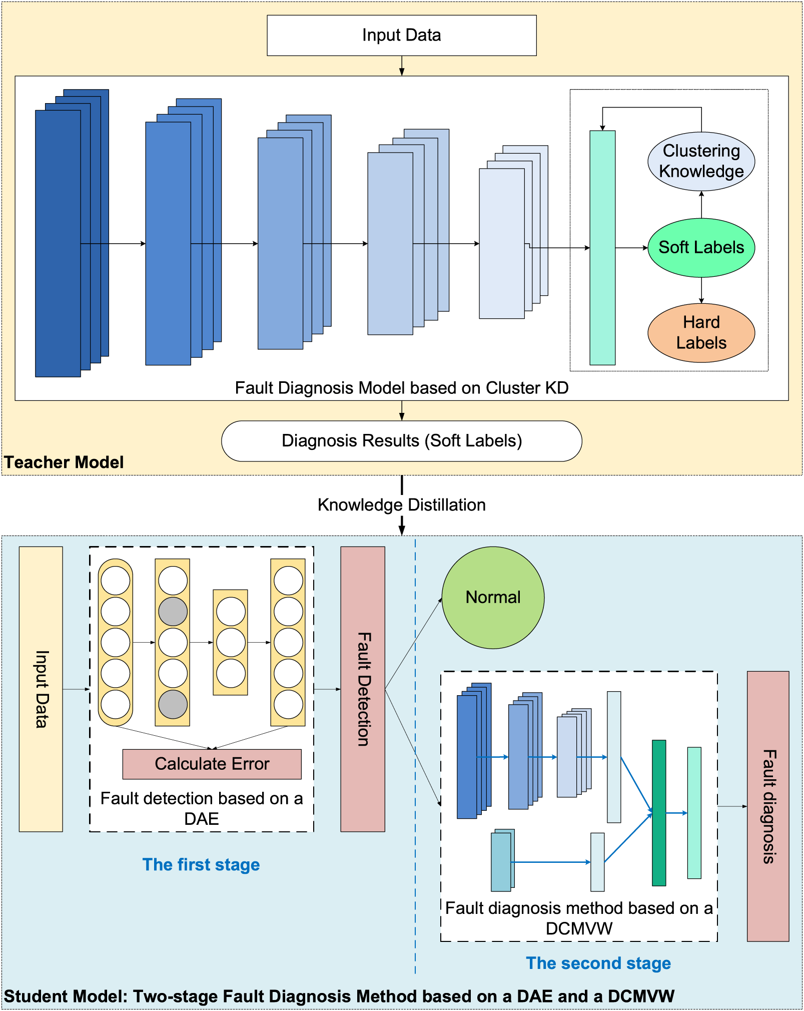
Figure 1: The structure of the proposed two-stage edge-side fault diagnosis method based ondouble KD

The algorithm works as follows:

(1) The teacher model is built on the clustering-based self-KD algorithm. The T-model calculates the mean of all samples in each class during training, taking the difference between each sample and the mean as part of the loss function. The T-model takes its output obtained through clustering calculation as knowledge to guide its training process. Then, the output of the original diagnosis performed by the T-model remains, namely, the soft labels. After building the student model, the soft labels are used as reference substance to guide the training process to improve the model accuracy during the process of KD.

(2) The student model is built based on the two-stage edge-side fault diagnosis method. A fault detection module based on a DAE and a fault diagnosis module based on a DCMVW is constructed in different stages. In fault detection, Gaussian noise is added to the input data. Then, the noisy data is encoded, decoded, and reconstructed. Finally, the calculation error is used to determine whether a fault is present. Then, the faulty data are entered into the fault diagnosis module, in which the fault features are extracted by convolution kernels of different sizes and concatenated. Finally, the probabilities of faults are calculated by classifiers, and the diagnosis results are output.

4.2 Double Knowledge Distillation Framework

In the edge-side fault diagnosis problem, the standard KD method can compress models, and self-KD can yield improved accuracy. However, how to effectively extract knowledge still needs to be solved. In this section, we describe a double KD framework, where the outer KD process is used to establish a knowledge transmission path from the T-model to the S-model via normal KD, and the internal KD process is utilized to establish the self-to-self way via clustering-based self-KD.

Reference [27] showed that the class-wise regularization loss is random in selecting the sampled input, which causes the loss fluctuations during training. A clustering-based self-KD (Cluster KD) method is proposed in this paper to smoothly realize knowledge iteration and reduce the confusion between different categories.

Because of the various correlations between each type of fault and the other types, the diagnostic probabilities of the same type are similar for all categories. This means that, to some extent, the fault data of two category A are more similar than that of one category A fault data and one category B fault data. The distribution of the diagnostic results obtained for samples in the same category should be consistent. Even if a prediction is wrong, it should be a similar mistake. Hence, during the training process, we make the diagnostic results of the same category tend to be consistent, reducing intra-class variations. We use clustering computing to measure the intra-class variations and normalize the results to achieve this. After each training epoch, the diagnostic results of all sample data for each category are averaged. This value is referred to as the “class center”. We then proceed to compute the distance between each sample and its corresponding class center, a technique known as ``intra-class regularization." To accomplish this, we employ the Kullback–Leibler (KL) divergence measure, which quantifies the difference between two distributions.

LKL(p||p¯)=∑i=1N⁡p(xi)(log⁡p(xi)p¯(xi))(5)

where p is the diagnosis result of a sample, p¯ is the current class center of the real sample category, p(xi) and p¯(xi) are the ith class probabilities of the sample diagnosis and the class center, respectively, and N is the total number of categories. The KL divergence is used to describe the difference between two distributions. It measures the difference between the class center and the class samples in this paper. This calculation method is similar to the clustering algorithm. Intra-class regularization can constrain the computational uniformity among samples of the same type. Furthermore, it can make the model perform stably for samples of the same class.

The intra-class regularization is taken as a term of the loss function:

LCLU−KD(p)=Lhard(p)+λcluLKL(p||p¯)(6)

where Lhard is the loss item with the original data label as a reference, and the hyperparameter λclu is the weight of the intra-class regularization process.

Through an experiment, we find that to make the model converge and avoid gradient explosion, λclu is recommended to satisfy the following condition:

s.t.Lhard(p)>λcluLKL(p||p¯)(7)

During model convergence, the data labels dominate the loss calculation. At the same time, the intra-class regularization only constrains the difference within each class, which works on the basis that the category with the maximum probability is calculated correctly. If intra-class regularization dominates the loss calculation, it will divert the model’s attention from the correct result. Hence, LKL(p||p¯) cannot be more influential than Lhard(p).

The above clustering algorithm is carried out in each round of iterative training. Since the constraint term of the calculation comes from the training process of the model itself and the model uses the learned knowledge to guide its training, it is called self-distillation. In the iterative process of cluster self-distillation, the model uses the mean value of diagnosis results as the constraint term, and the convergence is stable. Compared with the training method without clustering, the model strengthens the unity learning of the same category knowledge, reduces the possibility of outliers in the diagnosis results, and thus improves the accuracy.

The teacher model obtained after clustering-based self-KD improves the discrimination of different categories in the output knowledge. Then, we construct the outer KD process, in which the knowledge from the T-model is transferred to the S-model.

The knowledge transmission path of the double KD structure is shown in Fig. 2. Cluster KD (the T-model) outputs knowledge to guide its training process and then transmits it to the student model in the form of soft labels. The student model is introduced in the next section.

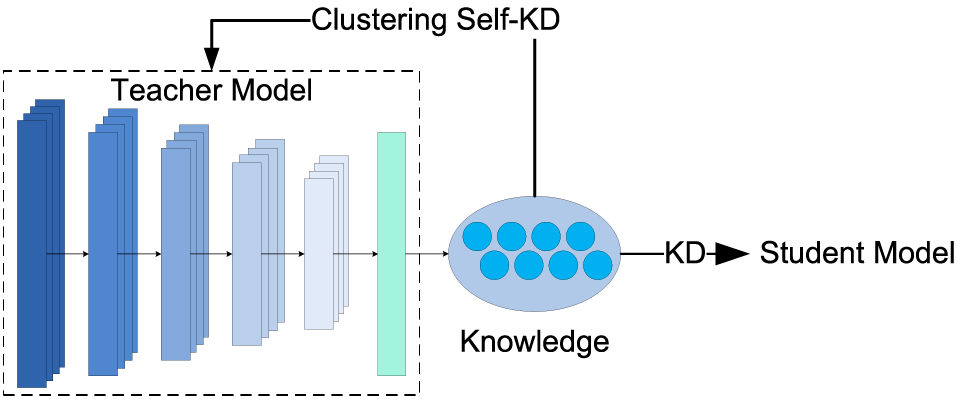
Figure 2: Transmission path of knowledge

4.3 Two-Stage Edge-Side Fault Diagnosis Method Based on a DAE and a DCMVW

In actual application scenarios, detecting and diagnosing massive data, including many fault-free data, is necessary to ensure normal operations. Most existing methods detect the existence and categories of faults, which means that the normal category and other faulty categories are treated as possessing equal importance. Performing complex diagnostics on normal data that typically occupy a larger volume can lead to significant computational and time consumption levels.

In this paper, a two-stage edge-side fault diagnosis method (TSM) based on a DAE and a DCMVW is designed as the student model of KD, as shown in Fig. 3. In the proposed way, fault detection and fault diagnosis are carried out in different stages: in the first stage, a fault detection model based on a DAE is adopted to achieve fast fault responses; in the second stage, a DCMVW is used to diagnose faults in detail. Since most data are detected as fault-free in the first stage, the fault diagnosis process is omitted in the second stage. Thus, the computational consumption is significantly reduced, and the time required to deal with faults is also reduced.

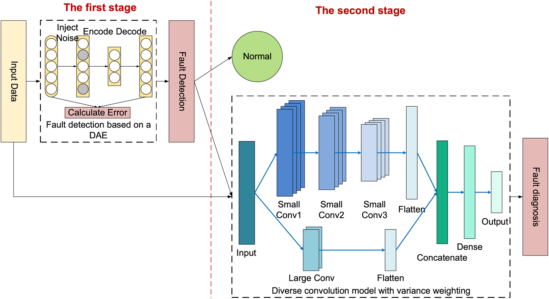
Figure 3: The structure of the two-stage edge-side fault diagnosis method based on a DAE and a DCMVW

The fault detection process in the first stage is a binary problem that only determines whether the given data are faulty. Compared with fault diagnosis, feature extraction for fault detection is easier because we do not need to identify specific faults. This paper adopts a fault detection method based on a DAE. The automatic encoder (AE) contains an encoder and a decoder, which are symmetric. Their purpose is to make the output and input as identical as possible. DAE injects noise into the clean input data so that the hidden layer can better capture input features and enhance the robustness of the model. It determines whether the input data are abnormal by performing dimensionality reduction and reconstructing it to calculate the reconstruction error. The structure of DAE is shown in Fig. 4.

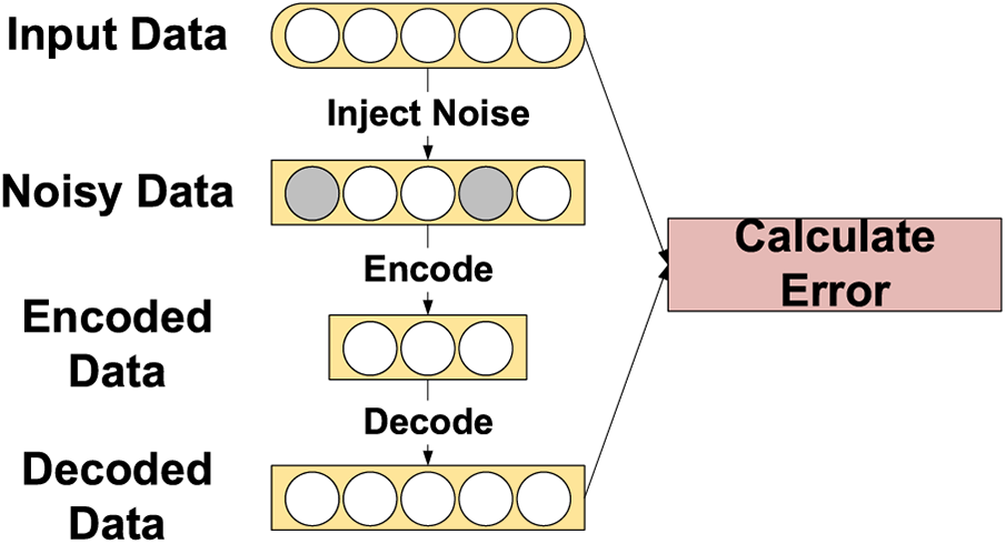
Figure 4: The structure of DAE

The working principles of a DAE are as follows:

1) Input Data: The DAE takes in raw input data.

2) Noise Introduction: To train the model to handle noise and extract meaningful features, the DAE introduces a certain level of random noise to the input data.

3) Encoder: The noisy input data is passed through an encoder network, which compresses and extracts features from the data. The encoder maps the input data to a low-dimensional representation known as the encoding.

4) Decoder: The output of the encoder is then fed into a decoder network. The decoder’s task is to reconstruct the encoding back to the original input dimensions, generating a reconstructed data output.

5) Reconstruction Error Minimization: By comparing the reconstructed data with the original input data, the reconstruction error is calculated. The objective of the DAE is to minimize this reconstruction error during training. This allows the model to effectively recover meaningful information from the input data while removing the noise components.

6) Feature Learning: During the training process, the DAE learns meaningful representations of the input data through the collaboration of the encoder and decoder. These representations capture important features in the data and can be utilized for various tasks such as classification, clustering, or generating new samples.

The raw input data are first injected with noise that follows a Gaussian distribution, as shown in Eq. (8).

f(x)=12πσexp⁡(−(x−μ)22σ2)(8)

where μ is the means and σ is the standard deviation.

The error between the original and rebuilt data is calculated by the mean squared error (MSE) metric to determine whether the data are abnormal. The calculation is performed as follows:

MSE=∑i=1n⁡(Yi−Y^i)2(9)

where n is the number of samples, Yi denotes the real values, and Y^i represents the predicted values.

The second stage is fine-grained fault diagnosis, where the data in which faults are found during the first phase undergo fault diagnosis. The classic fault diagnosis model Deep Convolutional Neural Networks with Wide First-Layer Kernels (WDCNN) [28] uses wide convolution to extract fault features and achieves good diagnosis results. Because of its wide field of view, the WDCNN must stack multiple convolutional structures, creating calculation pressure for device deployment. Currently, most models use wide convolution to process data like the WDCNN when processing sequential fault data. It focuses on the characteristics of the data in the long-time dimension and ignores the short-time dimension.

In this paper, considering the timing characteristics of fault data, a DCMVW is proposed, which uses two kinds of convolution kernels to extract fault features from different perspectives. The two sizes of convolution kernels focus on features from different angles of the data. Small convolution kernel extracts local microscopic features. After stacking multiple layers, it can extract stable features. Large convolution nuclei grasp the overall trend of data from a macro perspective and do not require multiple layers of convolution. The two features are connected in series to expand the vision of the model. Compared with a model possessing a single field of view, this model has a shallower depth and is less prone to overfitting and gradient problems. The size of the small convolution kernel used in this experiment is 5, and the size of the large convolution kernel is 64.

Some faults have similar characteristics and are difficult to distinguish accurately. This paper proposes a loss calculation method based on variance. For the training samples with unclear results, their loss weights are appropriately increased to make the model pay more attention to them. We measure the clarity of sample classification by the class probability variance, that is, the difficulty of classifying the given sample. The variance is used to assign a weight to the loss of this sample.

Suppose that the diagnosis probability of the model for each fault type is y′=(y1′,y2′,…,ym′), where m is the number of fault categories, and yi′ is the probability that a sample belongs to category i. Then, the variance of the probability of each type is

σp2=∑1m(y′−y′¯)2(10)

where y′¯ is the average value of yi′, as shown below:

y′¯=∑1myi′(11)

For a probability vector such as y′, a significant probability variance indicates a definite diagnosis. A definite diagnosis means that some fault is far more likely to occur than others and that the model is confident in its results. This also reflects the difficulty of classification. We conduct the following verification for the relationship between the class probability variance and classification difficulty. For an n-class probability vector, the result is usually the class with the highest probability. Suppose the maximum probability is denoted as x, at least 1/n, since it is the maximum value among all n possibilities. As x gradually approaches 1, the class probability variance increases. The general trend is shown in Fig. 5. The abscissa represents the extent to which the maximum probability is close to 1, meaning the classification difficulty. Fig. 5 only indicates the trends produced when the number of classes is 3, 5, and 9. This verifies that the more definite the diagnosis is, the more significant the variance.

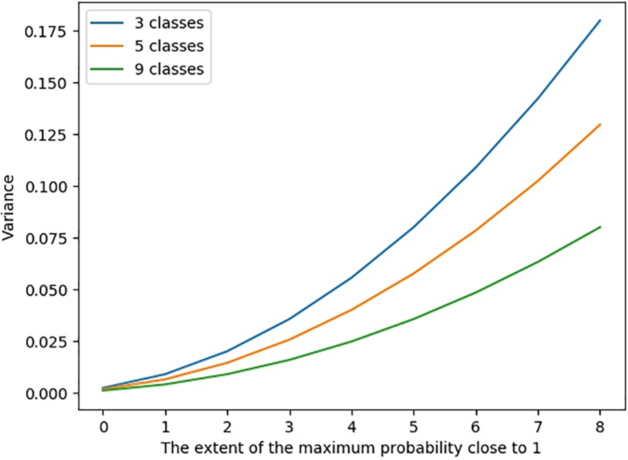
Figure 5: The class probability variance increases with the difficulty of sample classification

Based on the above analysis, samples with smaller probability variances are more difficult to diagnose, so their influence on the model should be improved. The loss function is defined as:

L=(1−σp2)⋅LCE(y,y′)(12)

LCE(y,y′)=−∑i=1n⁡∑j=1m⁡yij′log⁡yij(13)

where LCE represents the cross-entropy calculation.

The formula presented in Eq. (12) amplifies the weights assigned to challenging samples that are difficult to classify. Conversely, it reduces the weights of easily classifiable samples, thus exerting opposite influences on the adjustments of model parameters.

5  Experiments

5.1 Datasets

To investigate the effectiveness of the proposed two-stage edge-side fault diagnosis method based on double KD, we use two public datasets to conduct experiments in the paper:

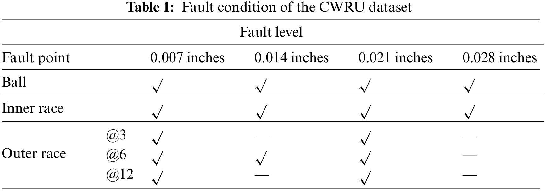
(1) Case Western Reserve University (CWRU) Bearing dataset [29]: The CWRU dataset includes vibration data of normal bearings and faulty bearings collected under four kinds of loads. The dataset contains properties of the condition and vibration signals that occur over time, with more than 120,000 time collection points for each fault condition. Their motor frequencies are 12 and 48 kHz, respectively. The data acquisition ends include the driver end and fan end. The fault points include the inner race, outer race, and rolling ball, among which the outer race has three points in the 3, 6, and 12 o’clock directions. There are four fault levels for a single point of failure: diameters of 0.007, 0.014, 0.021, and 0.028 inches.

In this paper, a total of 60 fault conditions, including three faulty parts under four loads, are selected. The 15 points and fault diameters, excluding their loads, are shown in Table 1.

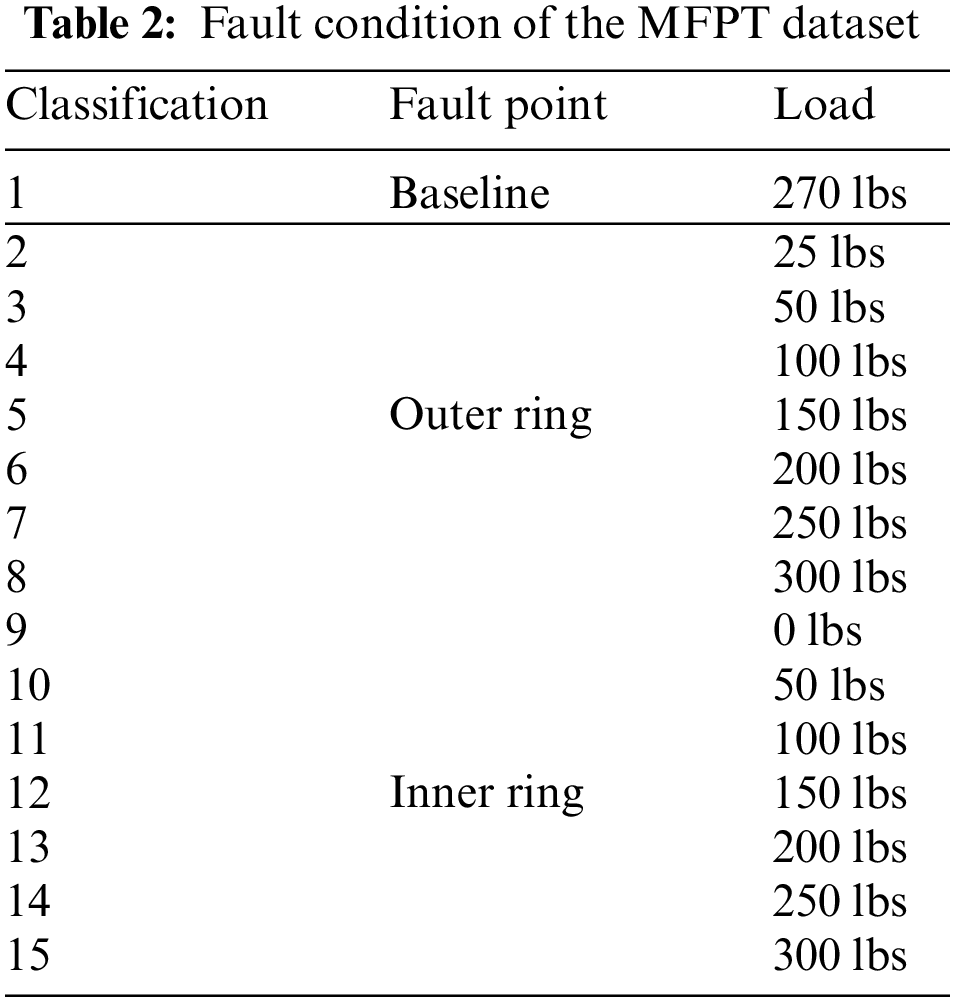
(2) MFPT dataset [6]: The MFPT dataset includes three baseline datasets, seven inner race faults, and seven outer race faults. In this case, the faults refer to the working conditions observed under different loads. The data set contains properties of the condition and vibration signals that occur over time, with more than 600,000 time collection points for each fault condition. In this paper, we use these conditions, with a total of 15 faults, and they are shown in Table 2.

The data is preprocessed before it is used to train and test the model. We divide the vibration signal sequence of hundreds of thousands of time points into sequence segments of 1024 time points and label them with fault categories. The input received by the model is a sequence of vibration signals at 1024 time points.

5.2 Baseline

In this paper, three methods developed in recent years are selected as comparison methods to provide strong support for proving the effectiveness of the proposed method:

(1) A neural network compression method based on knowledge-distillation and parameter quantization for the bearing fault diagnosis (DQSN) [30]: This method uses KD to improve the accuracy of the student network when training it. And then, the parameter quantization is conducted to compress the scale of the student network further. The paper, published in 2022, is one of the most superior fault diagnosis methods based on knowledge distillation.

(2) Vision ConvNet (VCN) [31]: This model can effectively increase the scope of network vision and improve the accuracy of model recognition by adding a small number of network parameters.

(3) Class-Wise Self-Knowledge Distillation (CS-KD) [27]: This method matches or distills the predictive distributions of Deep Neural Networks (DNN) among different samples with the same label, prevents overconfident predictions, and reduces intra-class variations.

5.3 Introduction to Computing Resources

The training experiment was performed on Windows 10 using Python and Keras based on Tensorflow. Table 3 describes the configuration of the environment.

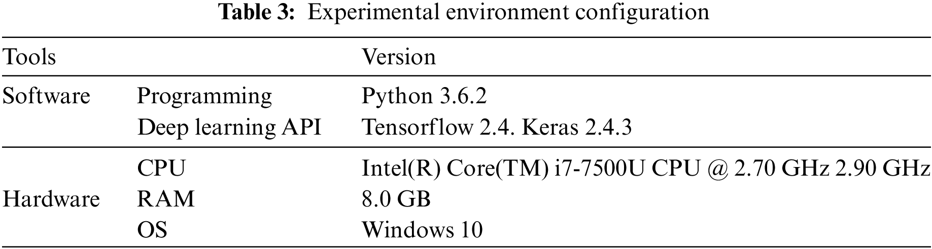
The trained model can be deployed on a Raspberry PI 4B with 2 G memory and a 1.5 GHz CPU. The weakening of hardware resources will extend the computing time. The subsequent experiments in this paper were carried out in the environment shown in Table 3.

5.4 Algorithm Parameters

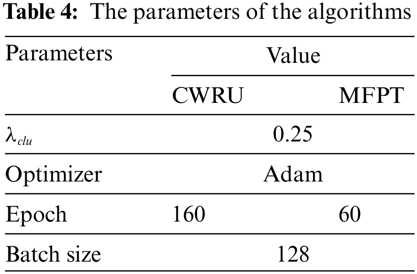
The parameters involved in this algorithm are shown in Table 4.

5.5 Evaluation Metrics

(1) Floating point operations (FLOPs): FLOPs are used to measure the computational complexity of a model and are often used as an indirect measure of the speed of a neural network model. This metric reflects the amount of model computation.

(2) Top-k accuracy: Top-k accuracy computes the number of times the correct label occurs among the top-k predicted labels. In this paper, we measure the accuracy achieved with k values of 1, 3,and 5.

(3) Precision, recall, and F1 score: The precision is the percentage of correctly labeled prediction results obtained by the model among all results, which reflects the accuracy of the model’s prediction results. The recall represents the percentage of the true results predicted by the model as a percentage of all outcomes. The F1 score is the harmonic average of precision and recall, representing the comprehensive performance of the tested prediction method regarding accuracy and recall. The precision, recall, and F1 score metrics are calculated as follows:

Precision=TPTP+FP(14)

Recall=TP TP+FN(15)

 F1=2⋅Precision⋅RecallPrecision+Recall(16)

where the true-positive (TP) rate is the number of correct diagnostic results, the false-positive (FP) rate is the number of faults that are diagnosed but do not exist, and the false-negative (FN) rate is the number of undiagnosed faults that exist.

5.6 Result Analysis

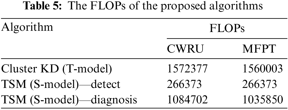
5.6.1 Results Analysis of the FLOP

The devices on the edge side are usually not equipped with powerful hardware, so we adopted the strategy of KD to compress our model. First, the FLOPs of the T-model and S-model are considered to compare their computational complexity levels and compression ratios. The FLOPs of Cluster KD (T-model) and the detection and diagnosis parts of TSM (the S-model) are shown in Table 5. Because of the classification difference between these models, their computational complexities on different datasets are slightly different. For the classification of all fault categories, the calculations required by the model compressed via KD are reduced by 17.18% and 16.52% on the CWRU and MFPT datasets, respectively, showing that TSM has a more significant computation advantage. The diagnosis computation for the fault-free data is omitted, saving 83.06% and 82.92% of the costs, respectively. The larger the proportion of normal data in the dataset is, the more computation resources can be saved by the proposed method. The results show that our method can save computation, which means the reduction of computing resources, storage resources, and delay.

5.6.2 Results Analysis of Accuracy

To verify the effectiveness of the method proposed in this paper, we conduct a comparative analysis of multiple accuracy indicators.

First, we compare the accuracy performance of the algorithms on the validation set as the number of training iterations increases. Table 6 and Fig. 6 show the relationship between the validation accuracy and the number of epochs on the CWRU dataset. The accuracy of Cluster KD and TSM is significantly higher than other algorithms. Our approaches demonstrate excellent convergence and accuracy.

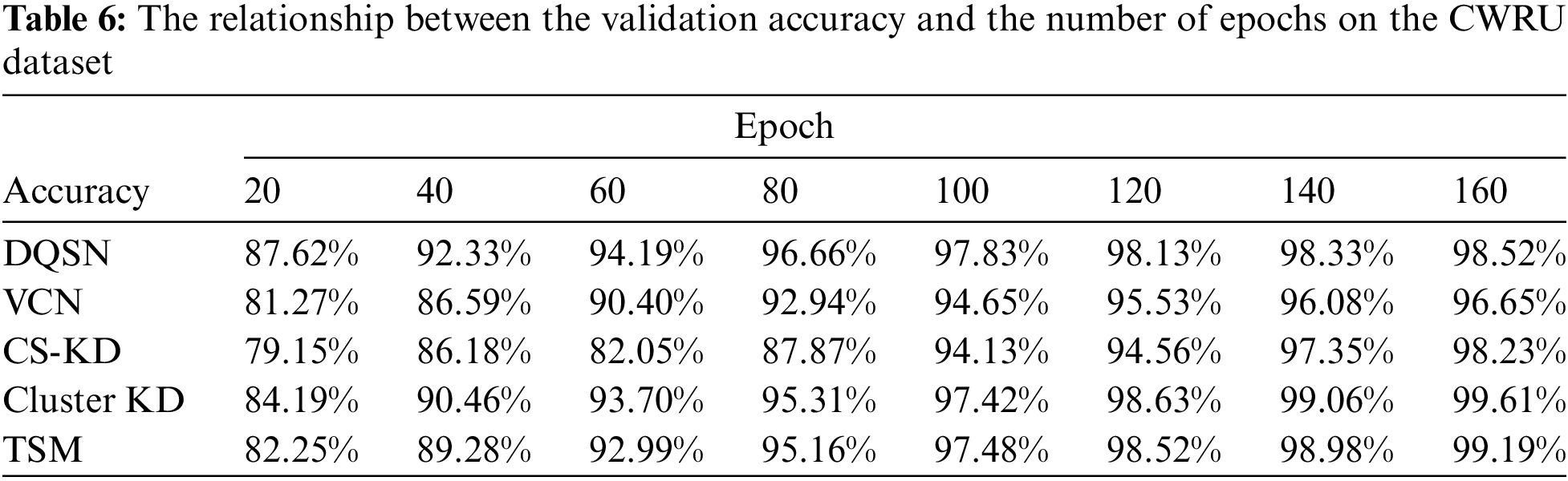
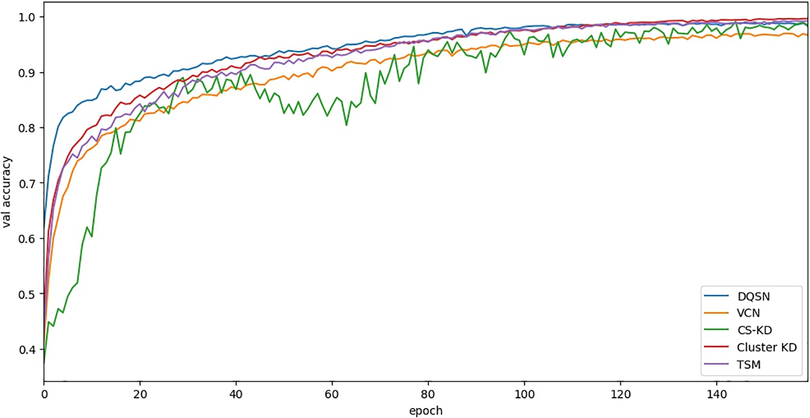
Figure 6: The curve between the validation accuracy and the number of epochs on the CWRU dataset

According to the relationships produced on the MFPT dataset and shown in Table 7 and Fig. 7, the five algorithms converge after approximately 50 to 60 epochs. The convergence of the five methods is similar, while our methods (Cluster KD and TSM) show higher accuracy. The specific results are further analyzed in the following experiments.

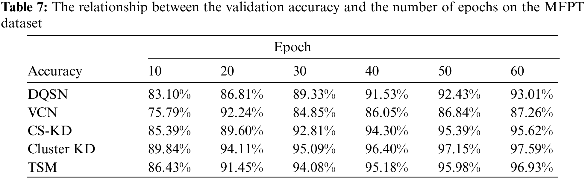
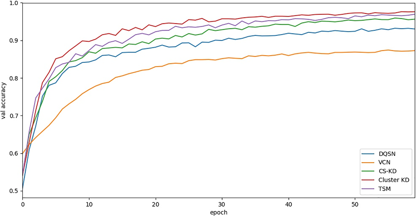
Figure 7: The curve between the validation accuracy and the number of epochs on the MFPT dataset

The above experiments verify the convergence and accuracy of our method by comparing it with different algorithms.

A confusion matrix is used to verify the classification effects yielded for fault categories with high similarity. According to reference [32], the CWRU dataset is easy to classify, while the MFPT dataset is challenging. Research shows that the classification effect of each method on the CWRU dataset is excellent, making it difficult to distinguish different methods. In addition, up to 60 fault categories are contained in this dataset, and the confusion matrix graph has difficulty effectively displaying information.

The confusion matrix produced for the MFPT dataset is shown in Figs. 7–11. The figures show significant differences among the observation conditions of all fault categories except category 0 (the normal category). Fig. 8 shows that Cluster KD has the best performance; its accuracy is below 0.95 only for categories 4, 5, and 9, where 4 and 5 are most likely to be confused. Fig. 9 shows that TSM achieves an effect close to that of Cluster KD; its accuracy is below 0.9 for categories 4, 5, and 8.

Figure 8: The confusion matrix produced by cluster KD (T-model) on the MFPT dataset

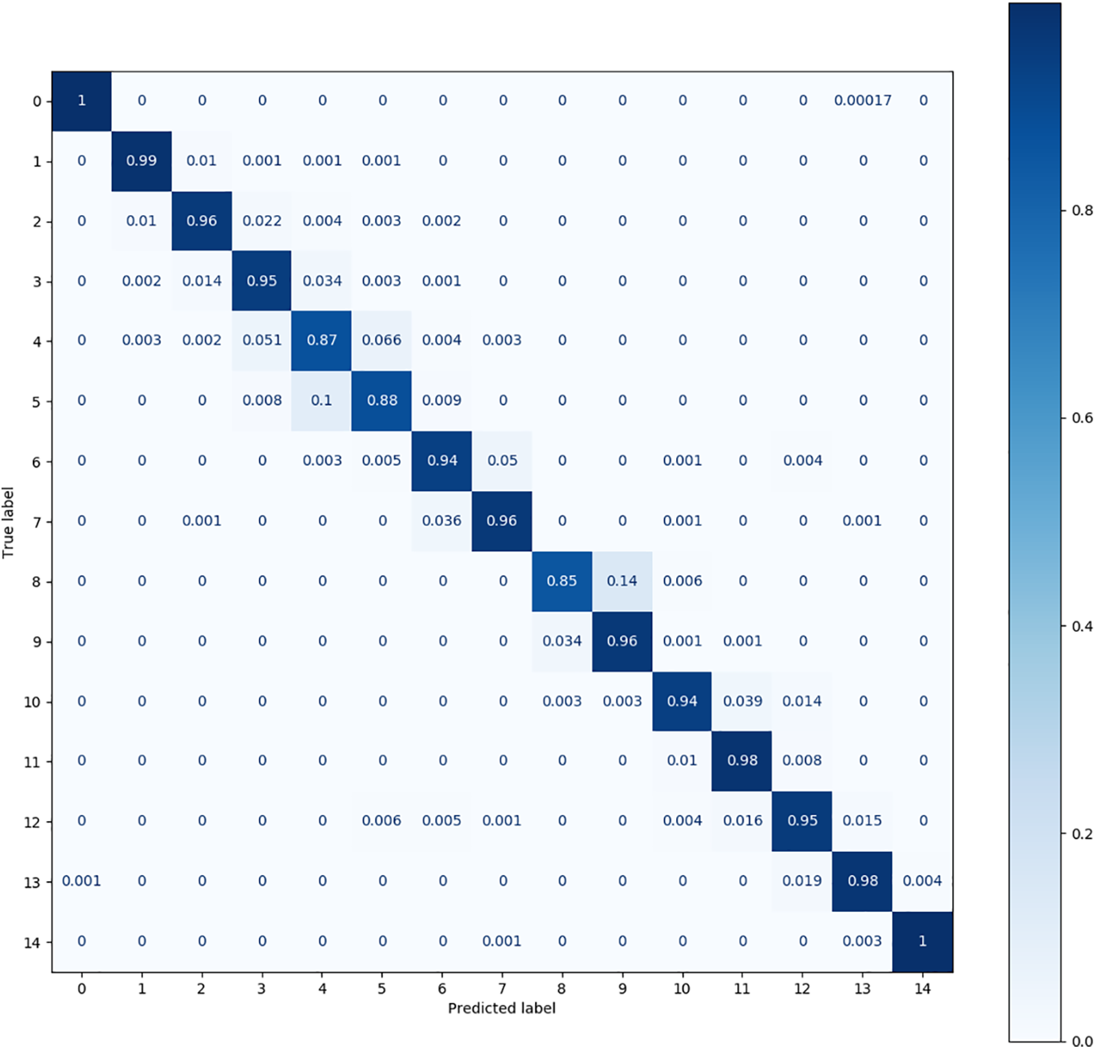
Figure 9: The confusion matrix produced by TSM (S-model) on the MFPT dataset

Figure 10: The confusion matrix produced by DQSN on the MFPT dataset

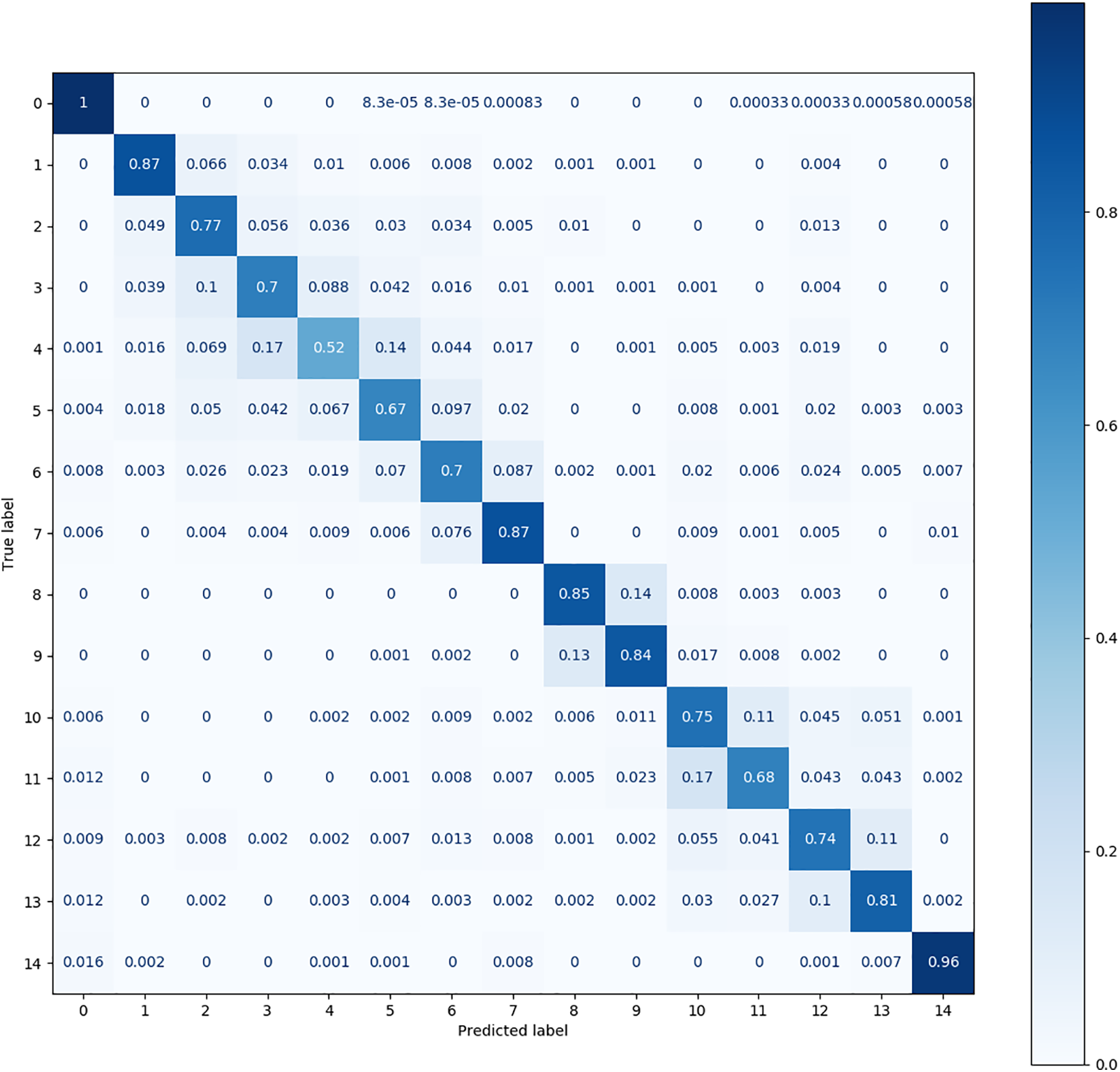
Figure 11: The confusion matrix produced by VCN on the MFPT dataset

Fig. 10 shows that the DQSN causes more confusion in more categories, achieving accuracies of 0.75 for category 4, 0.87 for category 5, 0.89 for category 6, and 0.86 for category 9. It yields the worst diagnosis for category 4. Fig. 11 shows that the confusion matrix of the VCN is the weakest; its accuracy is below 0.8 in as many as eight categories, among which the accuracy achieved for category 4 is only 0.52. Fig. 12 shows that CS-KD has inferior performance, with an accuracy below 0.9 for categories 3, 4, 5, 9, and 11. Upon comparing the situations of different categories, it can be seen that diagnosing categories 4, 5, and 9 is difficult for all algorithms. Our method significantly improves these categories, with an accuracy above 0.85. The performance of Cluster KD and TSM is excellent and balanced across all categories, with a slight particular preference for individual categories, indicating that our proposed method is more advantageous in distinguishing categories with high similarity.

Figure 12: The confusion matrix produced by CS-KD on the MFPT dataset

The top-k (k = 1, 3, 5) accuracy results are shown in Fig. 13. The Cluster KD method proposed in this paper achieves the best results on the three accuracy tests. The accuracies of Cluster KD on the CWRU and MFPT datasets reach 99.60% and 97.59%, respectively, which are 1.07% and 4.57% higher than those of the DQSN, 2.95% and 4.81% higher than those of the VCN and 1.37% and 1.96% higher than those of CS-KD. TSM also performs excellently; its accuracies reach 99.20% and 96.94% on the two datasets, which are also higher than those of the three comparison algorithms. Regarding top-3 accuracy, Cluster KD and TSM maintain their advantage but are reduced. On the CWRU dataset, the benefit is reduced to less than 0.1%. On the MFPT dataset, the top-3 accuracy of Cluster KD is 0.05%, 2.59%, and 0.05% higher than those of the DQSN, the VCN, and CS-KD, respectively. TSM achieves the same result as Cluster KD. From the above results, T and S achieve good precision values, which are better than those of the other three algorithms. As the k parameter of the top-k test increases, our method’s advantage decreases, indicating that our approaches have a more significant advantage when the diagnosis is performed only once and can identify faults better.

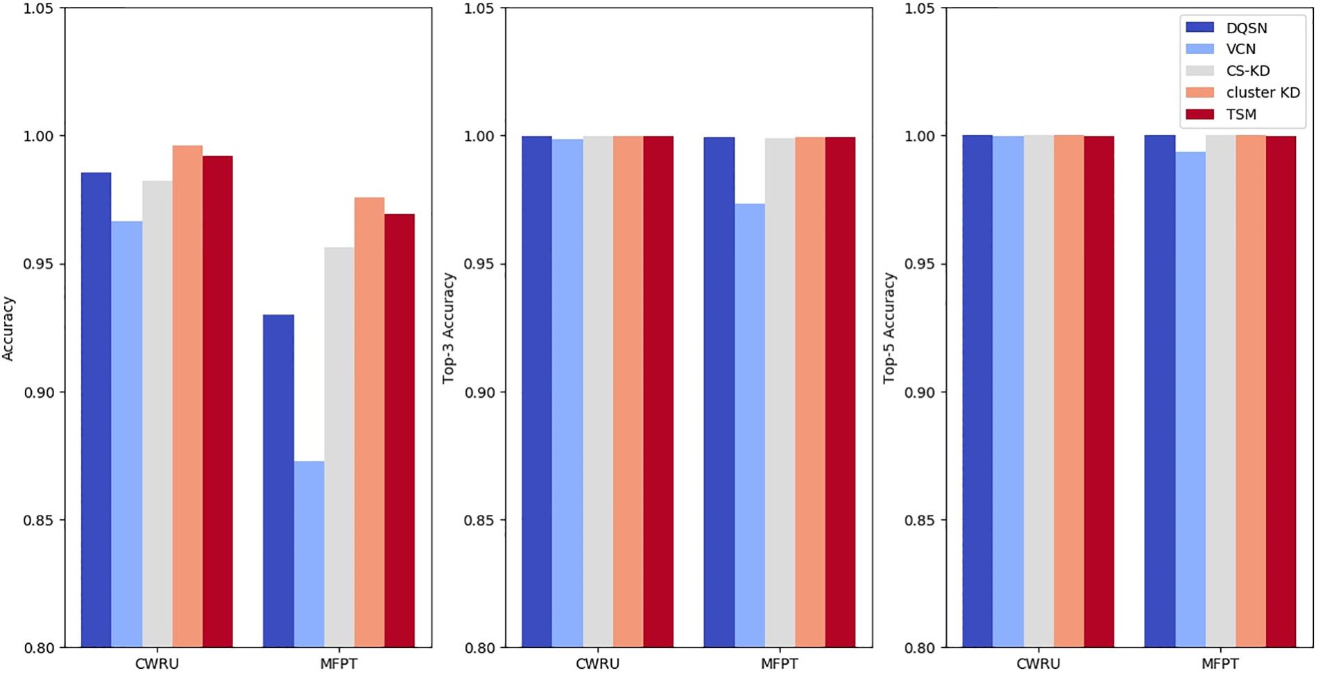
Figure 13: Top-k accuracy comparison

5.6.3 Result Analysis of Precision, Recall, and F1 Score Metrics

To further compare the performance of the algorithms, we calculate their precision, recall, and F1 values.

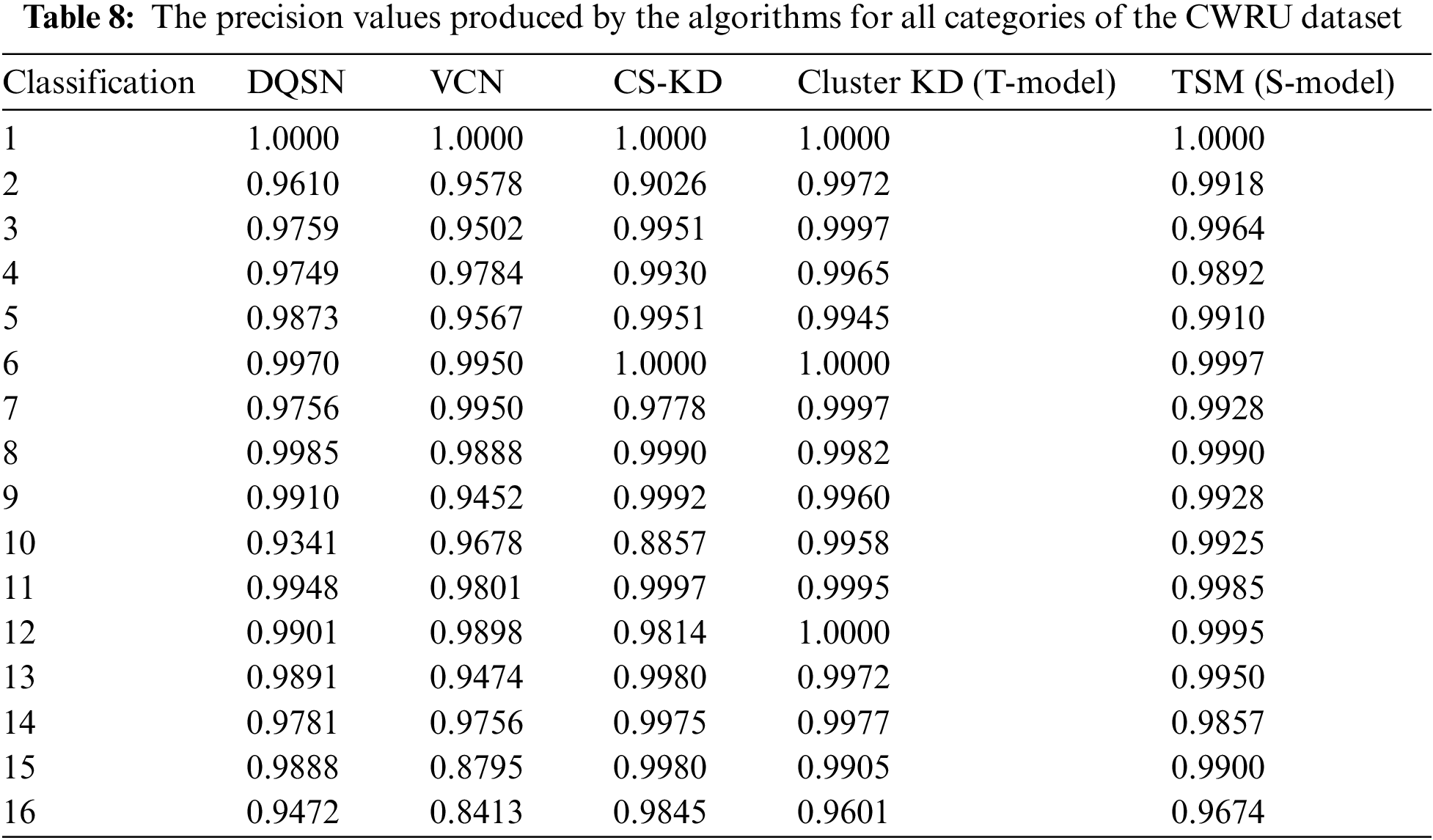
First, we compare the precision values achieved for each class of the two datasets. Since the CWRU dataset contains many categories, we combine the categories with the same conditions except their loads into one category, with 16 categories shown in Table 8. Cluster KD (the T-model) achieves the highest or near-highest results for almost all categories. TSM (the S-model) performs slightly worse than Cluster KD, with precision values of 0.05% to 0.6% lower for most categories. The DQSN performs well in categories 8 and 12. The precision of the VCN is as high as 0.995 for categories 5 and 6 but below 0.9 for categories 15 and 16. The precision of CS-KD is lower for categories 2 and 10 than for the other categories.

The precision results obtained for 15 categories of the MFPT dataset are shown in Table 9. Cluster KD and TSM perform weakly on categories 4, 5, 9, and 10, among which the precision values achieved for categories 4 and 5 are 0.9017/0.9202 and 0.8704/0.8573, respectively, on the two datasets. It is worth noting that the other algorithms perform even worse in categories 4 and 5: the precision values of the DQSN, the VCN, and CS-KD for category 5 are 0.8382, 0.6877, and 0.7695, respectively. This indicates that these two categories are difficult to classify, and our method greatly improves. The classification imbalance problem is evident in the MFPT dataset. The DQSN achieves precision values below 0.9 in categories 4, 5, 6, 8, and 9 and a value of only 0.7744 for category 9. The precision values produced by the VCN for most categories are lower than 0.9, indicating its weak feature extraction ability for difficult datasets. CS-KD performs weakly in categories 5, 6, 9, and 11. The improvement provided by our method is particularly evident in these difficulty categories. Compared with those of the DQSN, the VCN, and CS-KD, the precision values of Cluster KD and TSM are increased by 0.0294/0.2213/0.0051 and 0.0479/0.2398/0.0134, respectively, on category 4; 0.0322/0.1827/0.1009 and 0.0191/0.1696/0.0878 on category 5; 0.1545/0.0843/0.0558 and 0.1840/0.1138/0.853 on category 9; and 0.0635/0.2716/0.1256 and 0.0713/0.2794/0.1334 on category 11. The data above show that our methods can more easily identify difficult fault categories.

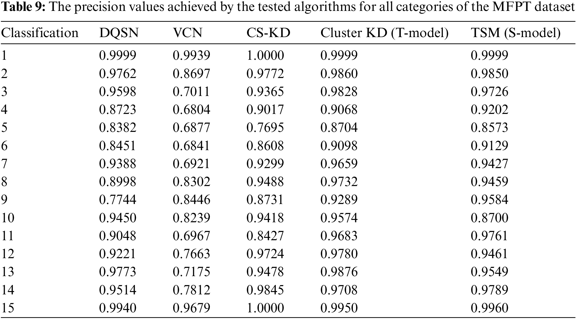
Compared with the other three algorithms, one of Cluster KD and TSM’s key advantages is their balanced and excellent performance across various categories. The other three models have high precision values in a few categories but have significant weaknesses. Cluster KD and TSM have high precision and good balance, with few preferences for specific categories. The experimental results further demonstrate the high accuracy and ability of our method to identify confounding faults.

The precision, recall, and F1 results are shown in Fig. 14. In terms of precision, Cluster KD reaches 99.61% and 97.71% on the two datasets, which are 1.07% and 5.41% higher than those of the DQSN, 2.76% and 6.92% higher than those of the VCN, and 1.37% and 1.70% higher than those of CS-KD, respectively. TSM reaches precision values of 99.21% and 97.14%, which are 0.67% and 4.85% higher than those of the DQSN, 2.36% and 6.35% higher than those of the VCN, and 0.96% and 1.14% higher than those of CS-KD. The results of TSM are 0.40% and 0.56% lower than those of Cluster KD concerning precision. In terms of recall, Cluster KD reaches values of 99.60% and 97.46% on the two datasets, which are 1.07% and 4.86% higher than those of the DQSN, 3.25% and 14.64% higher than those of the VCN, and 1.40% and 2.30% higher than those of CS-KD. TSM reaches recall values of 99.19% and 96.69%, which are 0.66% and 4.09% higher than those of the DQSN, 2.83% and 13.87% higher than those of the VCN, and 0.99% and 1.53% higher than those of CS-KD. The results of TSM are 0.41% and 0.76% lower than those of Cluster KD concerning recalls. In terms of F1, Cluster KD reaches values of 99.61% and 97.58% on the two datasets, which are 1.07% and 4.65% higher than those of the DQSN, 3.01% and 11.41% higher than those of the VCN, and 1.38% and 2.02% higher than those of CS-KD. TSM reaches F1 values of 99.20% and 96.91%, which are 0.67% and 3.98% higher than those of the DQSN, 2.61% and 10.74% higher than those of the VCN, and 0.98% and 1.35% higher than those of CS-KD. The results of TSM are 0.41% and 0.67% lower than those of Cluster KD concerning F1. Compared with Cluster KD (the T-model), the performance of TSM (the S-model) is slightly decreased in each indicator. However, it is still significantly better than the other algorithms. This demonstrates the effectiveness of the proposed method in the paper.

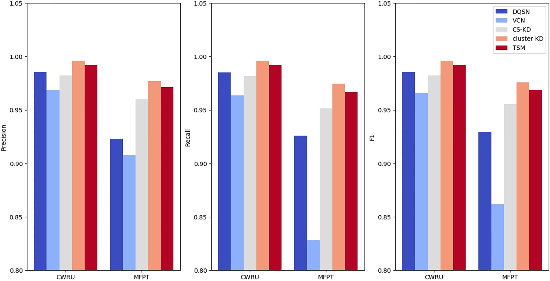
Figure 14: Precision, recall, and F1 metric comparisons

5.6.4 Result Analysis of the Ablation Study on TSM

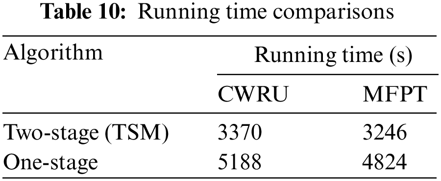
An ablation experiment is conducted to further verify the effectiveness of the two-stage in the student network. The running time of the two-stage and one-stage models is shown in Table 10. The running time is saved by 35.0% and 32.7% on the CWRU and MFPT datasets, which indicates that TSM can reduce computation consumption and speed up the diagnosis.

5.6.5 Comparison with State of Art

At present, there are few pieces of research on the application of knowledge distillation in the field of fault diagnosis, and there is a lack of recognized state of art. In order to compare with the most advanced methods, we select literature [30] as one of the comparison algorithms. The experimental results have been presented in this section. Experiments show that the accuracy of our method is 1.1% higher than that of this algorithm, and the ability to identify easily confused faults is better than that of this algorithm.

5.7 Limitation

Although our proposed method has achieved good experimental results, it still has some limitations. The study of fault diagnosis in this paper has the limitation of data, only the bearing fault data is used for experiments, and further exploration is needed in a wider range of fields. Due to the limitation of experimental equipment, the edge-side scenes targeted in this paper are single, and more edge-side devices need to be investigated in the future. The fault diagnosis method studied in this paper only supports the known fault categories, and the unknown faults cannot be classified and can only judge the anomalies. There is room to improve the generalization ability of the model.

6  Conclusion

This paper proposes a two-stage edge-side fault diagnosis method based on double KD. First, a clustering-based self-KD method is proposed, which utilizes the correlations between faults of the same type to improve the accuracy of the teacher model. Then, a double KD framework is constructed to build a lightweight model for edge-side deployment. Then, we propose a two-stage edge-side fault diagnosis method based on a DAE and a DCMVW as the student model. The model separates fault detection and fault diagnosis into different stages.

The proposed method has achieved advanced results in the research of fault diagnosis based on knowledge distillation and provides a new idea to apply the improved knowledge distillation to fault diagnosis. Experiments show that compared with other algorithms, the proposed method has significant advantages in computation and accuracy, especially in the ability to identify easily confused faults.

However, our approach still has limitations in terms of data, scenario applicability, generalization ability, and so on. Future research may consider the following directions:

1)   Study more edge-side failure scenarios, such as edge-side networks, Internet of Things devices, etc.

2)   The algorithm is improved so that it can identify unknown fault types.

Acknowledgement: Thanks to the researchers who have contributed to fault diagnosis and knowledge distillation in the past. The authors also gratefully acknowledge the helpful comments and suggestions of the reviewers, which have improved the presentation.

Funding Statement: This work is supported by the National Key R&D Program of China (2019YFB2103202).

Author Contributions: The authors confirm contribution to the paper as follows: algorithm conception and design: Yang Yang, Yuhan Long; experimental implementation and result analysis: Yang Yang, Yuhan Long; draft manuscript preparation: Yijing Lin, Zhipeng Gao, Lanlan Rui; proofreading of papers: Lanlan Rui, Peng Yu. All authors reviewed the results and approved the final version of the manuscript.

Availability of Data and Materials: The data used in this paper are presented in references [6] and [29].

Conflicts of Interest: The authors declare that they have no conflicts of interest to report regarding the present study.

References

1. B. D. Deebak and F. A. Turjman, “Digital-twin assisted: Fault diagnosis using deep transfer learning for machining tool condition,” International Journal of Intelligent Systems, vol. 37, no. 12, pp. 10289–10316, 2022. [Google Scholar]

2. M. Hussain, T. D. Memon, I. Hussain, Z. A. Memon and D. Kumar, “Fault detection and identification using deep learning algorithms in induction motors,” Computer Modeling in Engineering & Sciences, vol. 133, no. 2, pp. 435–470, 2022. [Google Scholar]

3. I. B. M. Taha and D. A. Mansour, “Novel power transformer fault diagnosis using optimized machine learning methods,” Intelligent Automation & Soft Computing, vol. 28, no. 3, pp. 739–752, 2021. [Google Scholar]

4. F. M. Shakiba, M. Shojaee, S. M. Azizi and M. Zhou, “Generalized fault diagnosis method of transmission lines using transfer learning technique,” Neurocomputing, vol. 500, no. 12, pp. 556–566, 2022. [Google Scholar]

5. D. K. Soother, S. M. Ujjan, K. Dev, S. A. Khowaja, N. A. Bhatti et al., “Towards soft real-time fault diagnosis for edge devices in industrial IoT using deep domain adaptation training strategy,” Journal of Parallel and Distributed Computing, vol. 160, no. 43, pp. 90–99, 2022. [Google Scholar]

6. Society for Machinery Failure Prevention Technology, 2023. [Online]. Available: https://mfpt.org/fault-data-sets/ [Google Scholar]

7. A. Ghani, M. Khanapi, M. A. Ibrahim, M. S. Mostafa, S. A. A. Ibrahim et al., “Implementing an efficient expert system for services center management by fuzzy logic controller,” Journal of Theoretical and Applied Information Technology, vol. 95, pp. 3127–3135, 2017. [Google Scholar]

8. M. A. Mohammed, M. K. A. Ghani, N. Arunkumar, O. I. Obaid, S. A. A. Mostafa et al., “Genetic case-based reasoning for improved mobile phone faults diagnosis,” Computers & Electrical Engineering, vol. 71, no. 42, pp. 212–222, 2018. [Google Scholar]

9. A. Lakhan, M. Elhoseny, M. A. Mohammed and M. M. Jaber, “SFDWA: Secure and fault-tolerant aware delay optimal workload assignment schemes in edge computing for Internet of drone things applications,” Wireless Communications and Mobile Computing, vol. 2022, no. 2, pp. 5667012–5667023, 2022. [Google Scholar]

10. Y. Kang, Y. Noh, M. Jang, S. Park and J. Kim, “Hierarchical level fault detection and diagnosis of ship engine systems,” Expert Systems with Applications, vol. 213, no. 5, pp. 118814, 2023. [Google Scholar]

11. E. Yu, L. Luo, X. Peng and C. Tong, “A multigroup fault detection and diagnosis framework for large-scale industrial systems using nonlinear multivariate analysis,” Expert Systems with Applications, vol. 206, no. 15, pp. 117859–117871, 2022. [Google Scholar]

12. D. Lan, M. Yu, Y. Huang, Z. Ping and J. Zhang, “Fault diagnosis and prognosis of steer-by-wire system based on finite state machine and extreme learning machine,” Neural Computing & Applications, vol. 34, no. 7, pp. 5081–5095, 2022. [Google Scholar]

13. L. H. P. Silva, L. H. S. Mello, A. Rodrigues, F. M. Varejão, M. P. Ribeiro et al., “Active learning for new-fault class sample recovery in electrical submersible pump fault diagnosis,” Expert Systems with Applications, vol. 212, no. 1, pp. 118508, 2023. [Google Scholar]

14. J. Yang, W. Bao, X. Li and Y. Liu, “Improved graph-regularized deep belief network with sparse features learning for fault diagnosis,” Neural Computing & Applications, vol. 34, no. 12, pp. 9885–9899, 2022. [Google Scholar]

15. J. Deng, W. Jiang, Y. Zhang, G. Wang, S. Li et al., “HS-KDNet: A lightweight network based on hierarchical-split block and knowledge distillation for fault diagnosis with extremely imbalanced data,” in Proc. IEEE Transactions on Instrumentation and Measurement, vol. 70, pp. 1–9, 2021. [Google Scholar]

16. X. Wang, A. Chen, L. Zhang, Y. Gu, M. Xu et al., “Distilling the knowledge of multiscale densely connected deep networks in mechanical intelligent diagnosis,” Wireless Communications and Mobile Computing, vol. 2021, pp. 12, 4319074, 2021. [Google Scholar]

17. N. Li, Y. Zhao, D. Li and W. Guan, “Real-time prediction of highway equipment faults based on GCN and GRU algorithms,” in Proc. of SMC, Melbourne, Australia, pp. 3252–3257, 2021. [Google Scholar]

18. J. Gou, B. Yu, S. J. Maybank and D. Tao, “Knowledge distillation: A survey,” International Journal of Computer Vision, vol. 129, no. 6, pp. 1789–1819, 2021. [Google Scholar]

19. F. Yuan, L. Shou, J. Pei, W. Lin, M. Gong et al., “Reinforced multi-teacher selection for knowledge distillation,” in Proc. of AAAI Conf. on Artificial Intelligence, vol. 35, no. 16, pp. 14284–14291, 2021. [Google Scholar]

20. Z. Wang, “Data-free knowledge distillation with soft targeted transfer set synthesis,” in Proc. of AAAI Conf. on Artificial Intelligence, vol. 35, no. 11, pp. 10245–10253, 2021. [Google Scholar]

21. X. Li, S. Li, B. Omar, F. Wu and X. Li, “ResKD: Residual-guided knowledge distillation,” in Proc. of IEEE Transactions on Image Processing, vol. 30, pp. 4735–4746, 2021. [Google Scholar]

22. C. Shen, X. Wang, Y. Yin, J. Song, S. Luo et al., “Progressive network grafting for few-shot knowledge distillation,” in Proc. of AAAI Conf. on Artificial Intelligence, vol. 35, no. 3, pp. 2541–2549, 2021. [Google Scholar]

23. G. Wu and S. Gong, “Peer collaborative learning for online knowledge distillation,” in Proc. of AAAI Conf. on Artificial Intelligence, vol. 35, no. 12, pp. 10302–10310, 2021. [Google Scholar]

24. Y. Wu, M. Rezagholizadeh, A. Ghaddar, M. A. Haidar and A. Ghodsi, “Universal-KD: Attention-based output-grounded intermediate layer knowledge distillation,” in Proc. of Conf. on Empirical Methods in Natural Language Processing, Online and Punta Cana, Dominican Republic, Association for Computational Linguistics, pp. 7649–7661, 2021. [Google Scholar]

25. M. Ji, S. Shin, S. Hwang, G. Park and I. C. Moon, “Refine myself by teaching myself: Feature refinement via self-knowledge distillation,” in Proc. of IEEE/CVF Conf. on Computer Vision and Pattern Recognition, Nashville, TN, USA, pp. 10659–10668, 2021. [Google Scholar]

26. K. Kim, B. Ji, D. Yoon and S. Hwang, “Self-knowledge distillation with progressive refinement of targets,” in Proc. of 2021 IEEE/CVF Int. Conf. on Computer Vision (ICCV), Montreal, QC, Canada, pp. 6547–6556, 2021. [Google Scholar]

27. S. Yun, J. Park, K. Lee and J. Shin, “Regularizing class-wise predictions via self-knowledge distillation,” in Proc. of 2020 IEEE/CVF Conf. on Computer Vision and Pattern Recognition (CVPR), Seattle, WA, USA, pp. 13873–13882, 2020. [Google Scholar]

28. W. Zhang, G. Peng, C. Li, Y. Chen and Z. Zhang, “A new deep learning model for fault diagnosis with good anti-noise and domain adaptation ability on raw vibration signals,” Sensors, vol. 17, no. 2, pp. 425–445, 2017. [Google Scholar] [PubMed]

29. Case Western Reserve University (CWRU) Bearing Data Center. [Online]. Available: https://engineering.case.edu/bearingdatacenter/download-data-file [Google Scholar]

30. M. Ji, G. Peng, S. Li, F. Cheng, Z. Chen et al., “A neural network compression method based on knowledge-distillation and parameter quantization for the bearing fault diagnosis,” Applied Soft Computing, vol. 127, no. 7, pp. 109331–109344, 2022. [Google Scholar]

31. Y. Wang, X. Ding, Q. Zeng, L. Wang and Y. Shao, “Intelligent rolling bearing fault diagnosis via vision ConvNet,” IEEE Sensors Journal, vol. 21, no. 5, pp. 6600–6609, 2021. [Google Scholar]

32. Z. Zhao, T. Li, J. Wu, C. Sun, S. Wang et al., “Deep learning algorithms for rotating machinery intelligent diagnosis: An open source benchmark study,” ISA Transactions, vol. 107, pp. 224–255, 2020. [Google Scholar] [PubMed]