A Spider Monkey Optimization Algorithm Combining Opposition-Based Learning and Orthogonal Experimental Design

1  Introduction

The real-world optimization problems are to select a group of parameters and make the design target reach the optimal value under a series of given constraints. It is well known that many optimization problems are comparatively hard to solve [1–4]. Nature-inspired optimization algorithms are part of the computer intelligence disciplines, which have become increasingly popular over the past decades [5]. A lot of optimization algorithms, such as Evolutionary Algorithm (EAs) [6], Particle Swarm Optimization (PSO) [7], Ant Colony Optimization (ACO) [8], Artificial Bee Colony (ABC) [9], Pigeon-Inspired Optimization Algorithm (PIO) [10], Slime Mould Algorithm (SMA) [11] and Crow Search Algorithm (CSA) [12] have been developed to deal with difficult optimization problems. These intelligent biological systems have similar characteristics in which the single individual behavior is simple and random, but the biological groups consisting of these individuals can cooperate to complete a series of complex tasks. Research shows that bionic algorithms can effectively handle numerous kinds of optimization problems.

Inspired by the food-searching behavior of spider monkeys, Bansal et al. developed a new bionic algorithm, called Spider Monkey Optimization (SMO) [13]. Since the SMO algorithm was proposed, this algorithm has been widely used in various complex optimization problems. It has been shown that it is superior concerning reliability, effectiveness, and accuracy to the regular ABC, Distribution Estimation Algorithm (DEA), PSO, and other intelligent algorithms. However, the SMO algorithm has some shortcomings. Typically, the new space exploration power of the original SMO is limited, i.e., it cannot eliminate the poor individuals in time and the diversity of the population is not abundant. These shortcomings seriously affect the performance of the SMO algorithm.

In this paper, we focus on how to reconstruct the SMO algorithm to improve its performance. We propose a spider monkey algorithm combining opposition-based Learning (OBL) and orthogonal experimental design (OED) to cope with unconstrained and constrained optimization problems. The main contributions of our work include: (1) A position update method based on historical optimal domains and particle swarm for Local Leader Phase (LLP) and Global Leader Phase (GLP) is developed. We introduce a novel position update method that combines the particle swarm and traditional update method so that the diversity of the population can be improved. In addition, the position update is performed in the dynamic domain composed by the optimal historical individual with a certain probability to make full use of historical search experience. (2) A population regeneration method based on Opposition-Based Learning (OBL) is presented. Different from other modified SMO algorithms, our approach does not directly enter the Local Leader Learning Phase (LLLP) stage after the LLP and GLP. Instead, it first uses the OBL strategy to avoid suffering from premature convergence and getting stuck at locally optimal values. (3) A method to eliminate the worst individuals in each group of the SMO algorithm based on the orthogonal experimental design is developed. This method performs the horizontal dividing and factor determination of the worst individuals in each group and the global optimal individuals to generate new individuals by orthogonal experimental design. The individuals obtained from this hybrid method retain the historical search experience of the best and the worst spider monkey, thereby enhancing the search performance.

The rest of this paper is organized as follows. Section 2 introduces the related work on the spider monkey optimization algorithm. A spider monkey algorithm named SMO3 that combines opposition-based learning and orthogonal experimental design for unconstrained optimization problems is presented in Section 3. Section 4 proposes a spider monkey algorithm for the constrained optimization problem based on SMO3. The experimental results of unconstrained functions, CEC2006 benchmark sets, and a few engineering optimization problems are presented in Section 5. Section 6 concludes this paper and points out future research work.

2  Related Work

In recent years, many variants of SMO have been studied to improve the performances of the original algorithms. Kumar et al. [14] introduced the golden section search method for the position update at the local leader and global leader phases. In [15], a new position update strategy in SMO is presented. The moving distance of a spider monkey at the LLP, the GLP, and the LLDP stages is determined by the individual fitness value. Sharma et al. [16] proposed a position update method based on the age of the spider monkey, which can improve the convergence speed of the SMO algorithm. Hazrati et al. [17] evaluated the size of the position update step according to the fitness value, allowing individuals with small fitness values to quickly approach the globally optimal individual. Gupta et al. [18] developed an improved SMO named constrained SMO (CSMO) for solving constrained continuous optimization problems. Results show that CSMO can obtain better results than DE, PSO, and ABC algorithms. In [19], the position of the worst individual is updated by the fitness of the leader of LLP and GLP and thus the local searchability of SMO is enhanced. Sharam et al. [20] proposed a new method to enhance the searchability of the SMO algorithm, which can find the promising search area around the best candidate solution by iteratively reducing step size. Xia et al. [21] developed a discrete spider monkey optimization (DSMO), which gives different update position methods for the discrete coding in LLP, GLP, and LLDP. However, how to further improve the effectiveness of the SMO algorithm still requires in-depth investigation.

Since the SMO algorithm was proposed, it has been widely applied to various complex optimization problems [22]. Mittal et al. [23] proposed an SMO-based optimization algorithm to improve the network lifetime for clustering protocols. Singh et al. [24] developed an improved SMO named MSMO algorithm to synthesize the linear antenna array (LAA). Results show that the proposed algorithm is an effective way to solve complex antenna optimization problems. Bhargava et al. [25] applied the SMO algorithm to optimize the parameters of the PIDA controller to achieve the optimal control of the induction motor. Cheruku et al. [26] presented an SMO-based rule miner for diabetes classification, and the experiment results show that the classification accuracy of the presented algorithm is better than ID3, CART, and C4.5. Priya et al. [27] proposed an improved SMO algorithm called BW-SMO, which is used for optimizing the query selection of the database. It was found that the proposed method can effectively improve data security. Darapureddy et al. [28] developed a new content-based image retrieval system based on the optimal weighted hybrid pattern. A modified optimization algorithm called improved local leader-based SMO was proposed to optimize the weight that maximizes the precision and recall of the retrieved images. Sivagar et al. [29] developed an improved SMO based on elite opposition and applied it to optimize cell selection with minimal network load. Rizvi et al. [30] presented a Hybrid Spider Monkey Optimization (HSMO) algorithm to optimize the makespan and cost while satisfying the budget and deadline constraints for QoS, and the results obtained show that the effectiveness of HSMO is better than that of the ABC, Bi-Criteria PSO, and BDSD algorithms. Mageswari et al. [31] developed an enhanced SMO-based energy-aware clustering scheme to prolong the network lifetime for wireless multimedia sensor networks.

Compared with some classical SMO algorithms, the proposed method in this paper can obtain the optimal solution more times by running multiple times on unconstrained functions, and the optimal solution has higher accuracy. Also, the algorithm in this paper successfully obtains a higher proportion of feasible and optimal solutions on constrained functions. It is shown that the proposed algorithm is easy to jump out of the local optima and higher solving accuracy.

3  Spider Monkey Algorithm for Unconstrained Optimization

Real-world optimization problems usually can be described as mathematical models of unconstrained functions or constrained functions [32–34]. In this section, we first propose a spider monkey algorithm named SMO3 that combines opposition-based learning (OBL) and orthogonal experimental design (OED) for unconstrained optimization problems.

3.1 Local Leader Phase Based on Historical Optimal Domain and Particle Swarm

The local Leader Phase (LLP) is an important stage in the SMO algorithm. In this phase, the position of a spider monkey will be updated according to the local optimum. Different from the position update method of other spider monkey algorithms in LLP, the SMO3 algorithm has two new position update methods in LLP: one is based on the historical optimal domain, and another is based on particle swarms. It compares the pros and cons of the positions obtained by both update methods. The better new position will be compared with the old position, and the position with the better fitness value will be adopted as the current position for a spider monkey.

Definition 1. Let G1 = (g11, g12, …, g1M), G2 = (g21, g22, …, g2M),…, Gn = (gn1, gn2,…,gnM) be n historically optimal individuals, and the historical optimal domain is defined as follows:

ldj=mini(gij)(1)

        and

udj=maxi(gij)(2)

where [ldj, udj] is the j-th component of the historical optimal domain, 1 ≤ i ≤ n.

The position update method based on the historical optimal domain not only retains the update method of the traditional SMO algorithm in the LLP stage but also adds a random generation of spider monkey positions in the historical optimal domain. This method allows the individual component values to be limited in the historical optimal domain with a higher probability. Thus, the search experience of the better individual could be used to find new solutions. The mathematical model of the update method in the SMO3 algorithm is as follows:

If U (0,1) ≥ pr, then

SMijnew=SMij+U(0,1)×(LLkj−SMij)+U(−1,1)×(SMrj−SMij)(3)

If U (0,1) < pr, then

SMijnew={ldj+U(0,1)×(udj−ldj)U(0,1)>crSMijelse(4)

where SMij is the position of the j-th component of the i-th spider monkey, U (0,1) is a random number in [0,1], pr is the perturbation rate of the SMO algorithm, LLkj is the j-th component of the local leader of the k-th group, while udj and ldj are the upper and lower bounds of the historical optimal domain, cr ∈ (0,1) and r ≠ i.

In this paper, we introduce a particle swarm-based update method for LLP. This update method enables the spider monkey algorithm to search the solution space in various ways, thus ensuring the diversity of individuals and avoiding the algorithm from falling into a local optimum too early. Let vij be the walking speed of the i-th spider monkey in the direction j, and the mathematical model of its updated is given by Eq. (5).

vij=gw×vij+c1×r1×(SMrj−SMij)+c2×r2×(LLkj−SMij)(5)

where gw is the inertia weight, c1, and c2 are the learning factors, r1 and r2 are random numbers in [0,1], and r ≠ i. The speed value range of a spider monkey in the direction j is [−msj, msj], where msj = (Uj − Lj) * 0.2, Lj and Uj are the lower and upper bounds of the j-th decision variables respectively. The walking speed of a spider monkey is calculated by the experience of the local leader and local group member’s experience, and a spider monkey can be led to a better position. According to the walking speed of spider monkey vij, the position SMij of the i-th spider monkey in the direction j is updated by Eq. (6).

SMijnew=SMij+vij(6)

The LLP algorithm based on the historical optimal domain and particle swarm is given in Algorithm 1. Let N be the population size and D be the dimension size, Algorithm 1 requires updating all components of each individual, and running the SMO algorithm once requires updating N individuals. Thus, the time complexity of Algorithm 1 is O(n2).

3.2 Global Leader Phase Based on Historical Optimal Domain and Particle Swarm

In the global leader phase, each spider monkey updates its position using the position of global leader as well as the local group individual’s experience. The traditional position update equation for this phase is given by Eq. (7).

SMijnew=SMij+U(0,1)×(GLj−SMij)+U(−1,1)×(SMrj−SMij)(7)

In addition to the traditional position update method, we present a position update method based on particle swarm in GLP. The position obtained by the particle swarm method is compared with the position obtained by Eq. (7), and the better one is adopted as a candidate position.

Let vij be the walking speed of the i-th spider monkey in the direction j, and the updated method of vij is given by Eq. (8).

vij=gw×vij+c1×r1×(SMrj−SMij)+c2×r2×(GLj−SMij)(8)

The walking speed of a spider monkey is determined by the experience of the global leader as well as the local group individua’s experience by Eq. (8), and a spider monkey has a chance to move to a better position.

According to the spider monkey’s walking speed, the position of the i-th spider monkey in the direction j is updated in the same way by Eq. (6). The GLP algorithm based on the historical optimal domain and particle swarm is shown in Algorithm 2. Let N be the population size and D be the dimension size, Algorithm 2 requires updating one component of each individual, and running the SMO algorithm once requires updating N individuals. Thus, the time complexity of Algorithm 2 is O(n).

3.3 OBL Strategy Based on Extreme Value

The main idea of Opposition-Based Learning (OBL) is to evaluate the feasible solution and its reverse solution, and the better solution is adopted by the individuals of the next generation. Since opposition-based learning was developed, OBL has been applied to various optimization algorithms, which is capable of improving the performance of these optimization algorithms to search for the problem solution [35]. To make better use of the search experience of each spider monkey, we propose an OBL strategy based on its extreme value and apply it to the SMO3 algorithm.

Definition 2. Let the number of spider monkeys in population G be NP, and the position of the i-th spider monkey is denoted as Xi = (xi1, xi2, …, xiD), 1 ≤ i ≤ NP, and bestit = (bi1, bi2, …, biD) is the optimal position of the i-th spider monkey when the algorithm is iterated to the t-th generation, we define the optimal domain based on the individual's extreme value as follows:

lzj=minj(bij)(9)

and

uzj=maxj(bij)(10)

where 1 ≤ i ≤ NP, 1 ≤ j ≤ D.

Definition 3. Let bestit = (bi1, bi2, …, biD) be the best position of the i-th spider monkey when the algorithm is iterated to the t-th generation, then its j-th component is updated by the OBL strategy with a certain probability, and its updating method is given by Eq. (11).

bestijnew=U(0,1)×(uzj+lzj)−bestij(11)

If bestijnew is out of its dynamic domain, we recalculate it according to Eq. (12).

bestijnew={lzj+U(0,1)×(uzj−lzj)U(0,1)<0.5Lj+U(0,1)×(Uj−Lj)else(12)

where U (0,1) is a random number in [0,1].

In this paper, we first construct the lower and upper bounds of decision variables based on their extreme values. Furthermore, opposition-based learning is applied to calculate the best position of a spider monkey with the upper and lower bounds. If the position obtained by OBL is better than the current position, it is used to replace the current position. The OBL based on its extreme value is shown in Algorithm 3, where NP is the number of spider monkeys, and Xi = (xi1, xi2, …, xiD) is the position of spider monkey i, 1 ≤ i ≤ NP. It is not difficult to see that Algorithm 3 is composed of two nested loops, thus the time complexity of Algorithm 1 is O(n2).

3.4 Worst Individual Elimination Mechanism Based on Orthogonal Experimental Design

Orthogonal experimental design (OED) is an important branch of statistical mathematics, based on probability theory, mathematical statistics, and the standardized orthogonal table to arrange the test plan [36]. It is another design method to study multiple factors and multiple levels. It selects some representative points from the comprehensive test according to the orthogonality. These representative points have the characteristics of uniform dispersion and comparability. OED is an efficient, fast, and economical method of experiment design. Using an orthogonal experiment design to incorporate heuristic algorithms is an effective way to improve the efficiency of heuristic algorithms [37,38].

Let the worst individual of the i-th group be worst = (w1, w2,…, wD), and the global leader is gbest = (g1, g2,…, gD). We first use the method presented in [37] to calculate the level of each component of the worst individual and the global leader. Let Li,k be the value of the k-th level of the i-th component, and S is the number of levels, and the calculation method of Li,k is given in Eq. (13).

Lik=min(wi,gi)+(max(wi,gi)−min(wi,gi))×k−1D−1(13)

where i = 1, 2, …, D, k = 1, 2, …, S.

Let the number of factors in the orthogonal experiment be F. In the process of constructing S horizontal orthogonal tables, if the number of components is small, each component can be directly used as a factor. In this case, the number of factors F = D. In case the value of D is large, if D is directly used as D factors, the number of orthogonal experiments will be too large, which can increase the complexity of the algorithm and the algorithm may run too slowly. For this reason, D components are divided into F groups to satisfy Eq. (14):

D=F×h+n(14)

where h = int(D/F), and n = D%F. The components contained in each group are as follows:

Di=(w(i−1)×h+1,…,wi×h)1≤i≤F(15)

D1,j=(L1,…,Lh,j)1≤j≤S(16)

After various level values of each factor are determined, the best level combination method is chosen according to the orthogonal experimental design method to obtain a new individual. If the new individual is better than the worst individual in the group, the worst individual will be replaced by the new individual. Otherwise, the new individual will not be adopted into the population.

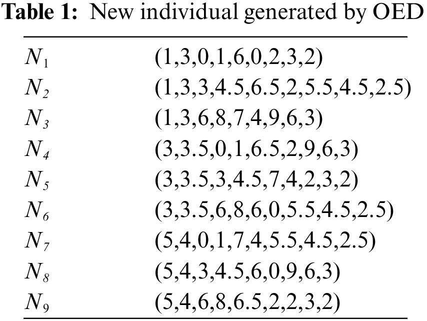
Finally, an example is presented to show how to use OED to generate new individuals based on the worst individual and the best individual. Let worst = (1,3,0,8,7,4,2,6,3) be the worst individual and gbest = (5,4,6,1,6,0,9,3,2) be the best individual in 9 dimensions space. The number of levels is 3, and the number of groups is 4. According to Eqs. (14) and (15), we have D1 = (x1,x2), D2 = (x3,x4), D3 = (x5,x6), and D4 = (x7,x8,x9). By Eq. (16), we can obtain 3 levels in each group as follows: D1,1 = (1,3), D1,2 = (3,3.5), D1,3 = (5,4), D2,1 = (0,1), D2,2 = (3,4.5), D2,3 = (6,8), D1,1 = (1,3), D1,2 = (3,3.5), D1,3 = (5,4), D3,1 = (6,0), D3,2 = (6.5,2), D3,3 = (7,4), D4,1 = (2,3,2), D4,2 = (5.5,4.5,2.5), and D4,3 = (9,6,3). Based on these data, we can apply orthogonal experimental design to generate new individuals. All individuals are given in Table 1.

3.5 Description of SMO3 Algorithm

The original SMO process consists of six phases: Local Leader Phase (LLP), Global Leader Phase (GLP), Global Leader Learning Phase (GLLP), Local Leader Learning Phase (LLLP), Local Leader Decision Phase (LLDP), and Global Leader Decision Phase (GLDP). The differences between the original SMO algorithm and the SMO3 algorithm that integration of OBL and orthogonal experiment design include: (1) In addition to the six phases of traditional SMO, it adds OBL and orthogonal experiment design stages. The implementation of these two stages is after LLP and GLP but before GLLP and LLLP. The addition of these two stages allows the group to generate new individuals in a variety of ways, thereby ensuring the diversity of the group. (2) The LLP and GLP stages of the algorithm in this paper are different from the traditional SMO algorithm. It adopts the local leader and global leader algorithms based on the historically optimal domains and particle swarms proposed in Sections 3.1 and 3.2. The flowchart of the SMO3 algorithm based on the fusion of OBL and orthogonal experimental design is shown in Fig. 1. The time complexity of the SMO3 algorithm is O ((n3 + n2 + n) Ngen + n2), where Ngen is the number of generations of the algorithm.

Figure 1: Flowchart of SMO3

4  SMO Algorithm for Constrained Optimization Problem

Different from the unconstrained optimization problem, the solution for the constrained optimization problems may not be the feasible solution, and the SMO3 algorithm cannot be used directly to solve the constrained optimization problem. For this reason, we extend the SMO3 algorithm to propose a spider monkey algorithm for dealing with constrained function optimization problems, namely CSMO3.

4.1 Evaluation of Individual’s Pros and Cons

It is well known that the pros and cons of the two individuals X1 and X2 in the search space are usually evaluated in the algorithm. For unconstrained optimization problems, if f(X1) < f(X2) X1 is better than X2. Otherwise, X2 is better than X1. In a constrained optimization problem, an individual in a search space may not be the feasible solution. Therefore, the evaluation of the individual’s pros and cons must be based on whether the individual is a feasible solution. We use the following rules to evaluate the individual’s pros and cons.

Rule 1: In case both individuals X1 and X2 are feasible solutions, if f(X1) < f(X2), then the individual X1 is better than X2, else X2 is better than X1.

Rule 2: If the individual X1 (X2) is a feasible solution, but X2 (X1) is not a feasible solution, the individual X1 (X2) is better than X2 (X1).

Rule 3: If both individuals X1 and X2 are not feasible solutions, the individual who violates fewer constraints is better than the individual who violates more constraints.

The judgment rule of Rule 3 is as follows: Let cn1 and cn2 be the numbers of individuals X1 and X2 that do not meet the constraints respectively, value(X1) < value(X2) be the violation constraint value of X1 and X2. If cn1 < cn2, the individual X1 is better than X2. If cn2 < cn1, the individual X2 is better than X1. When cn1 = cn2, if value(X1) < value(X2), the individual X1 is better than X2. Otherwise, X2 is better than X1. Different from the rule in [18] that only evaluates the pros and cons of individuals based on the violation constraint value, we give priority to individuals with a small number of violation constraints, and the pros and cons of the individual are determined by the violation constraint value only when cn1 is equal to cn2.

4.2 OBL Strategy of CSMO3 Algorithm

In the CSMO3 algorithm, the OBL strategy is used to generate the initial population to improve the quality of the initial population. Firstly, a population is randomly generated, and the OBL strategy is implemented to each decision variable of every individual by (17) with a certain probability.

xjnew=Lj+Uj−xj(17)

In addition to the OBL strategy for building the initial population, the population is also updated by the OBL strategy at each generation of the CSMO3 algorithm.

4.3 Local Leader Phase of CSMO3 Algorithm

In the local leader phase of the CSMO3 algorithm, a temporary new position is generated by the position update method of traditional LLP first. Next, the new position is updated by the particle swarm method with a probability of 0.4−cr so that another new position is obtained. Finally, the pros and cons of these new positions and the original position are compared by the evaluation rules in Section 4.1, and the best position is used to update the original position. The main steps of LLP are given in Algorithm 4.

Let N be the population size and D be the dimension size, Algorithm 4 requires updating all components of each two times, and running the SMO algorithm once requires updating N individuals. Thus, the time complexity of Algorithm 4 is O(2n2).

4.4 Global Leader Phase of CSMO3 Algorithm

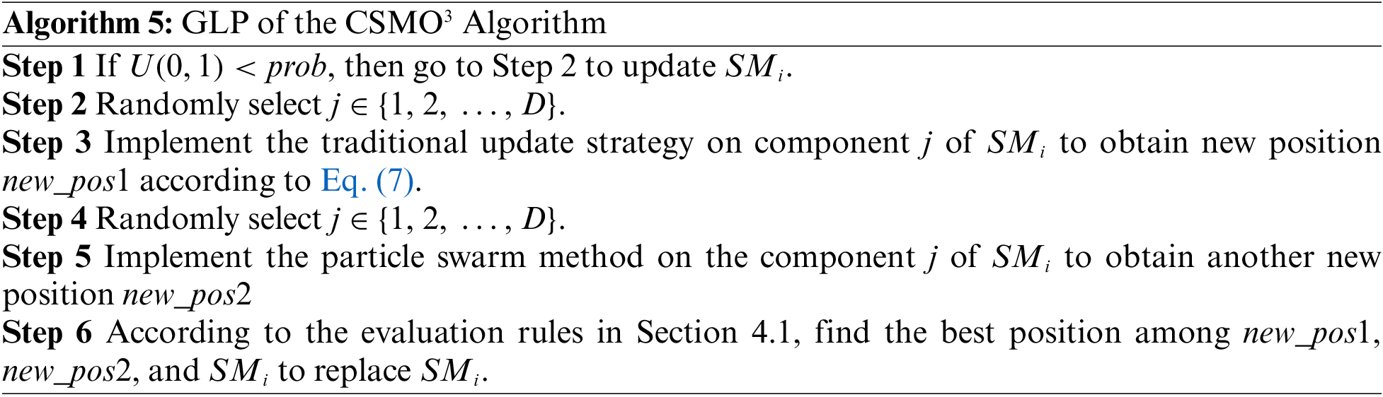
In the global leader phase of the CSMO3 algorithm, a temporary new position is generated according to the position update method of traditional GLP. Furthermore, a component of the new position is randomly selected to be updated according to the particle swarm method and obtain another new position. Finally, the pros and cons of these new positions and the original position are compared, and the best position is used to update the original position. The main steps of GLP are given in Algorithm 5. Let N be the population size and D be the dimension size, Algorithm 5 requires updating one component of each two times, and running the SMO algorithm once requires updating N individuals. Thus, the time complexity of Algorithm 5 is O(2n).

4.5 Description of CSMO3 Algorithm

The main steps of the CSMO3 algorithm for handling constrained optimization problems are similar to the main steps of the SMO3 algorithm in Section 3. The main differences include: (1) the OBL strategy is used to generate the initial population to improve the quality of the initial population in the CSMO3 algorithm; (2) the pros and cons of unfeasible solution are considered in the CSMO3 algorithm; (3) the CSMO3 algorithm only combines traditional position update method and particle swarm update method at LLP and GLP stage. The flowchart of the CSMO3 algorithm is shown in Fig. 2. The time complexity of the CSMO3 algorithm is O( (n3 + n2 + n) Ngen + n2).

Figure 2: Flowchart of CSMO3

5  Numerical Experiments

To verify the effectiveness of the spider monkey optimization algorithm proposed in this paper, the experiment comparison is performed on unconstrained functions, the CEC2006 benchmark set, and engineering examples. The proposed algorithm is coded in Python 3.2 and the experiments are run on a PC with Intel(R) Core(TM) i7-10510U, CPU @1.80 GHz 2.30 GHz, and Windows 10 operating system.

The parameter setting for every SMO algorithm has been adopted as it is mentioned in reference [15]. The parameter setting of SMO algorithms is as follows: the maximum number of generations of algorithms MIR = 20000, the population size N = 50, the number of groups MG = 5, GlobalLeaderLimit = 50, LocalLeaderLimit = 1500, the perturbation rate pr ∈ [0.1,0.4] with linear increase according to the number of iterations and prG+1 = prG + (0.4−0.1)/MIR. These parameters are currently recognized as the best combination of parameters for the SMO algorithm.

5.1 Experiments on Unconstrained Optimization Problems

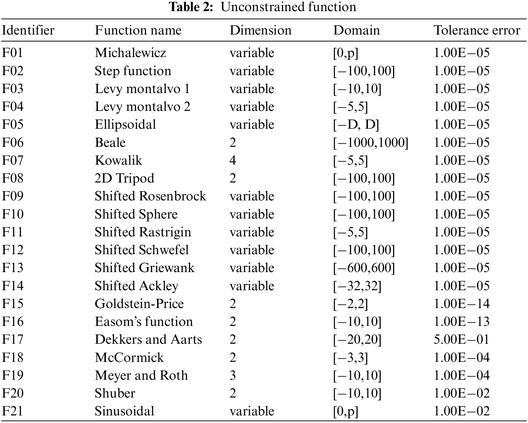
In this section, the effectiveness of the SMO3 algorithm is investigated. We use the SMO3 algorithm, original SMO algorithm [13], fitness-based position update in spider monkey optimization algorithm (FPSMO) [15], and adaptive step-size based spider monkey optimization algorithm (AsSMO) [17] to cope with unconstrained functions respectively. The results of SMO3 are compared with that of SMO, FPSMO, and AsSMO for performance demonstration. The classic test functions used in this section are briefly introduced in Table 2. Among 21 test functions, there are 12 functions with variable dimensions and 9 functions with fixed dimensions.

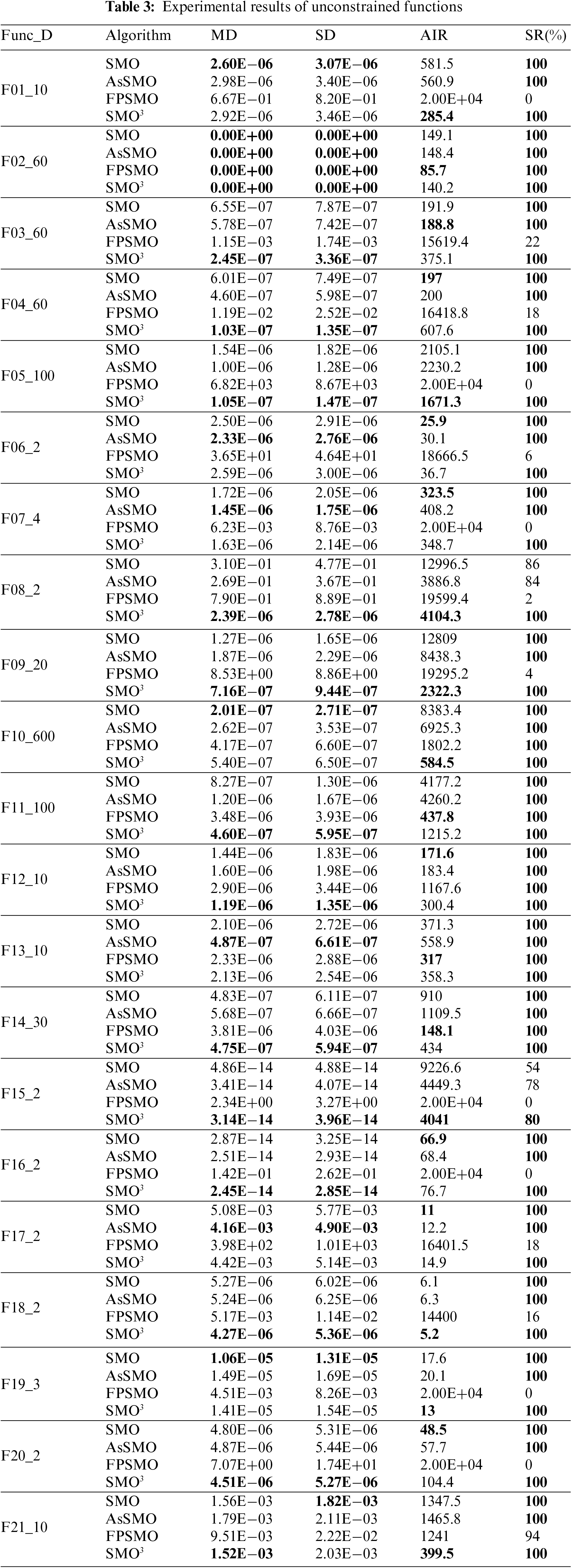
The accuracy of the results, the number of iterations, and the success rate of the four algorithms are compared in this section. Each algorithm runs 50 times on each function. Table 3 shows the experimental results which include the mean deviation (MD), standard deviation (SD), average number of iterations (AIR), and success rate (SR) of these 50 results. The success rate is the proportion of the results obtained from 50 runs of the algorithm within the tolerance error range. Among the 21 test functions, the success rate of the proposed method in this paper is higher than or equal to that of the other three algorithms. The success rate of the SMO3 algorithm is 100% except for function F15. F15 is the only function whose success rate of the four algorithms cannot reach 100%, where the success rates of SMO3, SMO, AsSMO, and FPSMO were 80%, 54%, 78%, and 0%, respectively. The mean deviation of the SMO3 algorithm on 14 functions is better than or equal to the other three algorithms, and SMO, AsSMO, and FPSMO algorithms have 4 functions, 5 functions, and 1 function, respectively. The standard deviation of the SMO3 algorithm on 13 functions is better than or equal to the other three algorithms, while SMO, AsSMO, and FPSMO algorithms have 5 functions, 5 functions, and 1 function respectively. The average number of iterations of the SMO3 algorithm on 9 functions is better than that of the other three algorithms, while SMO, AsSMO, and FPSMO algorithms only have 7 functions, 1 function, and 4 functions, respectively.

To compare the pros and cons of the above four algorithms comprehensively, the accuracy, average number of iterations, and success rate of each algorithm on 21 test functions are evaluated statistically for the number ranked 1st to 4th according to the experimental results in Table 3. Let x1, x2, x3, and x4 be the numbers of the algorithm ranked 1st to 4th in the index, and their score calculation method is given in Eq. (18).

score=x1+2x2+3x3+4x4(18)

The experimental results are shown in Table 3 and the comprehensive score of MD, SD, AIR, and SR is shown in Fig. 3. The smaller the comprehensive score, the more the number of rankings at the top. The number of 1st rankings in the MD, SD, AIR, and SR indicators for the SMO3 algorithm is 14, 13, 9, and 21, respectively; the comprehensive scores are 36, 29, 40, and 21, respectively; the comprehensive rankings of four indexes are all No. 1.

Figure 3: Score of MD, SD, AIR, and SR

The experimental results show that the SMO3 algorithm is more effective than SMO, AsSMO, and FPSMO in coping with unconstrained optimization problems. That is because the position update method based on PSO can increase the diversity of the population, opposition-based learning can enhance the ability to explore new space, and the method of eliminating the worst individual based on orthogonal experimental design can eliminate the worst individual in time.

5.2 Experiments on Constrained Optimization Problems

To examine the effectiveness of the CSMO3 algorithm in solving the constrained function optimization problems, the experiment is conducted on the CEC2006 benchmark set [39], which compares with the SMO algorithm, the AsSMO algorithm, and the FPSMO algorithm. These four algorithms use the same individual pros and cons evaluation method, and the main parameter settings are the same as in Section 5.1. Each algorithm runs 30 times. The feasible solution rate (FR), the best solution (BS), the worst solution (WS), the average solution (AV), the average number of iterations (AIR), and the success rate (SR) are respectively examined. The feasible solution rate is the ratio of obtaining the feasible solution in 30 runs, and the success rate is the ratio of obtaining the best-known solution in 30 runs. In the experiments on the CEC2006 benchmark set, the tolerance error is 1E-05 for g01, 1E-03 for g24, 1E-16 for both g08 and g12, and the tolerance errors of other functions are all 1E-04. The experimental comparison data on the CEC2006 benchmark set is shown in Table 4, where the bold data of each index indicates that the corresponding algorithm ranks first in this index, and ‘Vn’ means that the number of constraint violations is n.

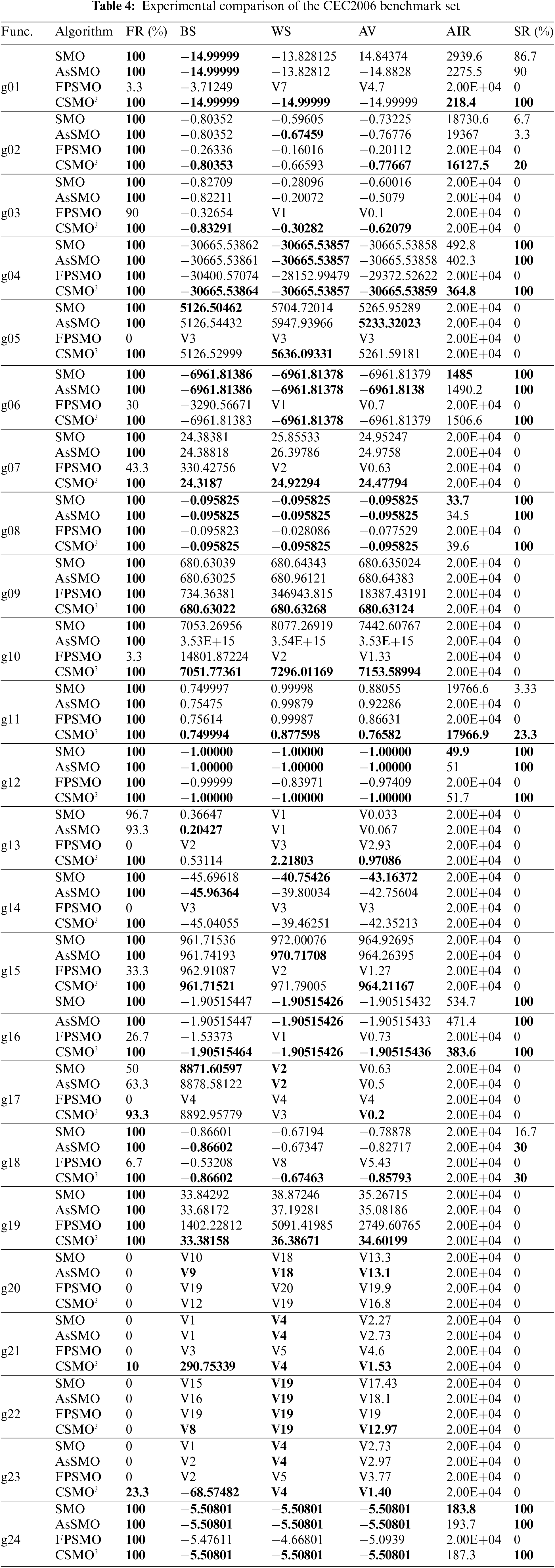
For function g01, the algorithm proposed in this paper can obtain the known optimal solution in each solution and its success rate is 100%. The success rates of SMO, AsSMO, and FPSMO algorithms are 86.7%, 90%, and 0%, respectively.

For function g02, the feasible solution rate of the four algorithms is 100%, but the success rate of the CSMO3 algorithm is higher than that of the other three algorithms.

The known optimal solution of g03 is −1.00050. However, none of these four algorithms can obtain the known optimal solution. The feasible solution rate of CSMO3 algorithms is 100% and the BS, WS, and AV of CSMO3 algorithms are better than that of the other three algorithms.

For g04, the success rate of the CSMO3 algorithm is 100% and the BS, WS, AV, and AIR of CSMO3 algorithms are better than that of the other three algorithms.

The known optimal solution of g05 is 5126.49671. The best solution of SMO, AsSMO, and CSMO3 are 5126.50462, 5126.54432, and 5126.52999 respectively. These solutions are close to the known optimal solution. For the average solution, AsSMO is better than CSMO3. The BS of SMO is better than CSMO3. The WS of CSMO3 is better than that of SMO, AsSMO, and FPSMO.

For g06, the FR, BS, WS, AV, and SR of SMO, AsSMO, and CSMO3 are almost equal. The AIR of SMO is better than AsSMO and CSMO3.

The known optimal solution of g07 is 24.30621. Except for FPSMO, the FR of the other three algorithms is 100%. The best solution of the CSMO3 algorithm is 24.31870, and the difference between this value and the known optimal solution is only 0.01249. The results show that CSMO3 is better than the other three algorithms.

For g08, the experiment results of SMO, AsSMO, and CSMO3 are equal except for the AIR. The AIR of SMO is better than AsSMO and CSMO3.

The known optimal solution of g09 is 680.63006. The SMO, AsSMO, and CSMO3 can find the solution, which is almost equal to the known optimal solution, where the best solution of the CSMO3 algorithm is 680.63022. The BS, WS, and AV of CSMO3 are better than that of the other three algorithms.

The known optimal solution of g10 is 7049.248021. The best solution of SMO, AsSMO, FPSMO, and CSMO3 is 7053.26956, 3.52952E+15, 14801.87224, and 7051.77361, respectively, where the BS of the CSMO3 algorithm is less than the value of other algorithms. In addition, the worst solution of CSMO3 is 7296.01169, which is better than that of the other algorithms.

For g11, all the algorithms can find a feasible solution in each solution. However, the SR of these algorithms is the smallest. The SR of CSMO3 is 23.3% and it is better than the BS of the other algorithms.

For g12, the experiment results of SMO, AsSMO, and CSMO3 algorithms are equal except for the AIR. The AIR of SMO, AsSMO, and CSMO3 are 49.9, 51, and 51.7, respectively.

The known optimal solution of g13 is 0.053942. None of these four algorithms can obtain the known optimal solution. The feasible solution rate of SMO, AsSMO, FPSMO, and CSMO3 is 96.7%, 93.3%, 0%, and 100%, respectively. CSMO3 is the only algorithm that can find a feasible solution in each run.

The known optimal solution of g14 is −47.76489. The feasible solution rates of SMO, As SMO, FPSMO, and CSMO3 are 100%, 100%, 0%, and 100%, respectively, but these four algorithms cannot obtain the known optimal solution. The BS, WS, and AV of CSMO3 are worse than those of SMO and AsSMO.

The known optimal solution of g15 is 961.71502. The best solution of CSMO3 is 961.71521, and the difference between this value and the known optimal solution is 0.00019. The WS of AsSMO is better than the WS of CSMO3, but the BS and AV of CSMO3 are better than the other algorithms.

For function g16, the success rate of CSMO3 is 100% and the BS, WS, AV, and AIR of CSMO3 are better than that of the other three algorithms.

The known optimal solution of g17 is 8853.53967. None of these four algorithms can obtain the known optimal solution. The feasible solution rates of SMO, AsSMO, FPSMO, and CSMO3 algorithms are 50%, 63.3%, 0%, and 93.3%, respectively. The average number of constraint violations of CSMO3 is 0.2, which is better than the other algorithms. The BS of the SMO algorithm is 8871.60597. This value is better than the BS of CSMO3.

For g18, the FR, BS, WS, AV, and SR of CSMO3 are equal to or better than the other algorithms.

The known optimal solution of g19 is 32.65559. None of these four algorithms can obtain the known optimal solution, but these algorithms can all find a feasible solution. The BS, WS, and AV of the CSMO3 algorithm are better than SMO, AsSMO, and FPSMO.

A feasible solution for g20 is not found so far. AsSMO can find solutions that violate 9 constraints and the average number of constraint violations of AsSMO is 13.1. In this function, the performance of AsSMO is better than SMO, FPSMO, and CSMO3.

The known optimal solution of g21 is 193.72451. SMO, AsSMO, and FPSMO cannot find feasible solutions. The FR of CSMO3 is 10% and the best solution of CSMO3 is 290.75339. The performance of the CSMO3 algorithm is better than that of the other algorithms.

The known optimal solution of g22 is 236.43098. None of these four algorithms can find a feasible solution. CSMO3 algorithm can find solutions that violate 8 constraints, and the average number of constraint violations is 12.97. In this function, the performance of CSMO3 is better than the other algorithms.

The known optimal solution of g23 is −400.05510. SMO, AsSMO, and FPSMO cannot find feasible solutions. The FR of CSMO3 is 23.3% and the best solution of CSMO3 is −68.57482. The performance of CSMO3 is better than other algorithms in function g23.

For function g24, the experiment results of SMO, AsSMO, and CSMO3 are equal except for the AIR. The AIR of SMO, AsSMO, and CSMO3 are 183.8, 193.7, and 187.3, respectively.

Experiment results show that the proposed algorithm in this paper is better than SMO, AsSMO, and FPSMO. The FR of CSMO3 in 24 test functions is equal to or better than the other three algorithms. It is noted that the FR of CSMO3 in g13, g17, g21 and g23 are 100%, 93.3%, 10%, and 23.3%, respectively. These data are better than the FR of SMO, AsSMO, and FPSMO. Moreover, the SR of the CSMO3 algorithm is not worse than the other three algorithms in each test function. For the BS of CSMO3, the BS of five functions is equal to the other algorithms, the BS of 13 functions is better than the other algorithms and only the BS of six functions is worse than other algorithms. In the WS of CSMO3, the WS of eight functions is equal to other algorithms, the WS of 10 functions is better than other algorithms, and only the WS of six functions is worse than the other algorithms. For the AV of CSMO3, the AV of three functions is equal to other algorithms, the AV of 17 functions is better than other algorithms, and only the AV of four functions is worse than other algorithms.

5.3 Experiments on Engineering Optimization Problems

To further verify the effectiveness of the CSMO3 algorithm, the spring tension design problem and the pressure pipe design problem are considered. The optimal solution of the CSMO3 algorithm is compared with the solution results of related algorithms in [40,41].

5.3.1 Spring Tension Design

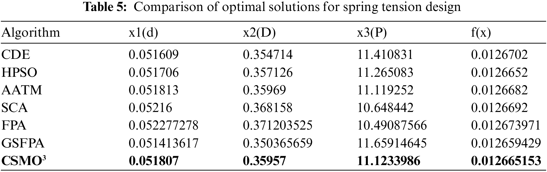
The optimization of spring tension design is to minimize the weight, when the three decision variables of the spring coil diameter, the average diameter of the spring coil, and the number of coils need to meet a set of constraints. The mathematical model of this problem is described by Eq. (19).

minf(x)=x12x2(2+x3)

s.t.{g1(x)=1−x3x2371785x14≤0g2(x)=4x22−x1x212556(x13x2−x14)+15108x12−1≤0g3(x)=1−140.45x1x23x3≤0g4(x)=x1+x21.5−1≤00.05≤x1≤20.25≤x2≤1.32≤x3≤15(19)

where the coil diameter is denoted by x1, the average diameter of coils is denoted by x2, and the number of coils is denoted by x3.

The comparison of solution results is shown in Table 5. The results show that the optimal solution of the CSMO3 algorithm proposed in this paper is 0.012665153339, which is better than the optimal solution of those algorithms used to compare with the flower pollination algorithm based on the gravitational search mechanism (GSFPA) presented in [40]. The result of the CSMO3 algorithm is only worse than GSFPA.

5.3.2 Pressure Pipe Design

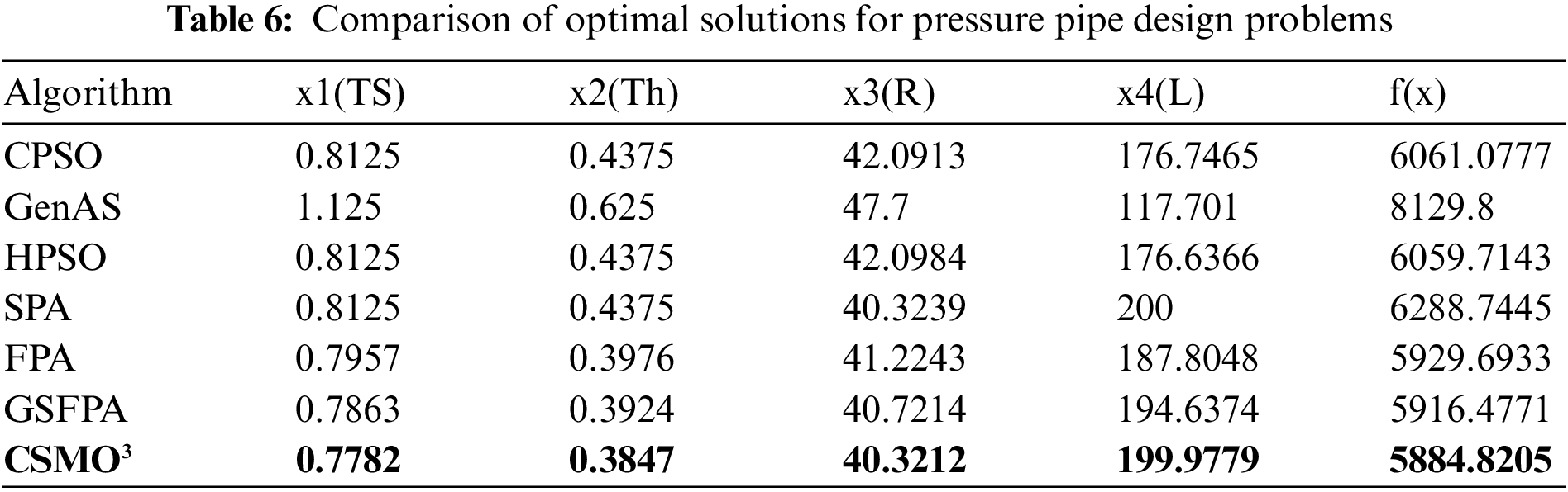
Optimization of pressure pipe design is to minimize the costs when four decision variables of cylindrical pipe thickness, hemispherical pipe thickness, cylindrical pipe inner diameter, and cylindrical pipe length must meet a few constraints. The mathematical model of this problem is as follows:

minf(x)=0.6224x1x3x4+1.7781x2x32+3.1661x12x4+19.84x12x3

s.t.{g1(x)=−x1+0.0193x3≤0g2(x)=−x2+0.00954x3≤0g3(x)=−πx32x4−4πx333+1296000≤0g4(x)=−240+x4≤00≤x1,x2≤10010≤x3,x4≤200(20)

where cylindrical pipe thickness is denoted by x1, the hemispherical pipe thickness is denoted by x2, the cylindrical pipe inner diameter is denoted by x3, and the cylindrical pipe inner diameter is denoted by x4.

The comparison of solution results is shown in Table 6. The optimal solution of the CSMO3 algorithm is 5884.8205, which is 31.6566 smaller than the optimal solution 5916.4771 of the GSFPA algorithm [40] and is better than the optimal solution of those heuristic algorithms used to compare with GSFPA presented in [40]. Thus, it can be found that the CSMO3 algorithm proposed in this paper is also effective in dealing with engineering optimization problems.

5.3.3 Parameter Estimation for Frequency-Modulated (FM) Sound Waves

The mathematical model of this problem is shown in [41]. There are six dimensions to optimize the FM synthesizer parameter. This issue is highly complex and multimodal, with strong episodic nature. In theory, the function value of the optimal solution to this problem is equal to zero.

Inspired by the Gorilla group and their social way of life in nature, a new metaheuristic algorithm called Artificial Gorilla Troops Optimizer (GTO) has been developed [41]. In optimizing the FM synthesizer parameter, a GTO can find high-quality solutions. The optimal solution of GTO is [−1.0000, −5.0000, 1.5000, 4.8000, 2.000, 4.9000], and the function value is 2.2811E−27. By using the CSMO3 algorithm to solve the problem, another optimal solution [0.9999, 5.0000, 1.5000, −4.7999, −2.0000, 4.8999] can be obtained, corresponding to the function value of 2.3583E−17. The optimization results of engineering problems show that the algorithm proposed in this paper performs also better than those heuristic algorithms used to compare with GTO presented in [41].

6  Conclusions and Future Work

This paper developed an improved method for the spider monkey algorithm. Because the position of a spider monkey determines the solution, how to update the position of the spider monkey plays a crucial role in problem-solving. A new updating method based on historical optimal domains and particle swarm was developed and population diversity can be improved. Also, this paper applied the OBL strategy to the traditional spider monkey algorithm. The proposed method can increase the individual diversity in the iterative process to avoid prematurely falling into the local optima. Furthermore, A method to eliminate the worst individuals in each group of the SMO algorithm based on the orthogonal experimental design is developed. The experiments on the classical unconstrained functions, constrained functions of the CEC2006 benchmark set, and engineering examples show that the optimization ability of the proposed algorithm is significantly better than other SMO and some evolution algorithms.

The method proposed in this paper has good performance in solving continuous function optimization problems. However, the spider monkey position update method cannot effectively describe the change of the solution for a combinatorial optimization problem, so the algorithm cannot effectively solve a combinatorial optimization problem. In the future, one direction worth exploring is how to build a spider monkey position update method suitable for combinatorial optimization problems, and then improve the ability of SMO to solve combinatorial optimization problems.

Acknowledgement: We would like to thank the editor and reviewers for their valuable comments, which are very helpful in improving the quality of the paper.

Funding Statement: This research was supported by the First Batch of Teaching Reform Projects of Zhejiang Higher Education “14th Five-Year Plan” (jg20220434), Special Scientific Research Project for Space Debris and Near-Earth Asteroid Defense (KJSP2020020202), Natural Science Foundation of Zhejiang Province (LGG19F030010), and National Natural Science Foundation of China (61703183).

Author Contributions: The authors confirm contribution to the paper as follows: study conception and design: W. Liao, X. Xia, H. Zhuang; data collection: X. Jia, X. Zhang; analysis and interpretation of results: X. Jia, S. Shen, H. Zhuang; draft manuscript preparation: X. Xia, S. Shen, H. Zhuang. All authors reviewed the results and approved the final version of the manuscript.

Availability of Data and Materials: Data will be made available on request from the corresponding authors.

Conflicts of Interest: The authors declare that they have no conflicts of interest to report regarding the present study.

References

1. S. Feng, L. Zhao, H. Shi, M. Wang, S. Shen et al., “One-dimensional VGGNet for high-dimensional data,” Applied Soft Computing, vol. 135, pp. 110035, 2023. [Google Scholar]

2. Y. Shen, S. Shen, Z. Wu, H. Zhou and S. Yu, “Signaling game-based availability assessment for edge computing-assisted IoT systems with malware dissemination,” Journal of Information Security and Applications, vol. 66, pp. 103140, 2022. [Google Scholar]

3. L. Kong, G. Li, W. Rafique, S. Shen, Q. He et al., “Time-aware missing healthcare data prediction based on ARIMA model,” IEEE/ACM Transactions on Computational Biology and Bioinformatics, Early Access, 2022. https://doi.org/10.1109/TCBB.2022.3205064 [Google Scholar] [PubMed] [CrossRef]

4. G. Wu, H. Wang, H. Zhang, Y. Zhao, S. Yu et al., “Computation offloading method using stochastic games for software defined network-based multi-agent mobile edge computing,” IEEE Internet of Things Journal, 2023. https://doi.org/10.1109/JIOT.2023.3277541 [Google Scholar] [CrossRef]

5. H. Ma, S. Shen, M. Yu, Z. Yang, M. Fei et al., “Multi-population techniques in nature inspired optimization algorithms: A comprehensive survey,” Swarm and Evolutionary Computation, vol. 44, pp. 365–387, 2019. [Google Scholar]

6. A. Rahman, R. Sokkalingam, O. Mahmod and K. Biswas, “Nature-Inspired metaheuristic techniques for combinatorial optimization problems: Overview and recent advances,” Mathematics, vol. 9, pp. 2633, 2021. [Google Scholar]

7. H. Shi, S. Liu, H. Wu, R. Li, S. Liu et al., “Oscillatory particle swarm optimizer,” Applied Soft Computing, vol. 73, pp. 316–327, 2018. [Google Scholar]

8. J. Liu, Y. Wang, G. Sun and T. Pang, “Multisurrogate-assisted ant colony optimization for expensive optimization problems with continuous and categorical variables,” IEEE Transactions on Cybernetics, vol. 53, no. 11, pp. 11348–11361, 2022. [Google Scholar]

9. Y. Xu and X. Wang, “An artificial bee colony algorithm for scheduling call centres with weekend-off fairness,” Applied Soft Computing, vol. 109, pp. 107542, 2021. [Google Scholar]

10. G. Chen, J. Qian, Z. Zhang and S. Li, “Application of modified pigeon-inspired optimization algorithm and constraint-objective sorting rule on multi-objective optimal power flow problem,” Applied Soft Computing, vol. 92, pp. 106321, 2020. [Google Scholar]

11. F. S. Gharehchopogh, A. Ucan, T. Ibrikci, B. Arasteh and G. Isik, “Slime mould algorithm: A comprehensive survey of its variants and applications,” Computational Methods in Engineering, vol. 30, pp. 2683–2723, 2023. [Google Scholar]

12. A. Saxena, “An efficient harmonic estimator design based on augmented crow search algorithm in noisy environment,” Expert Systems with Applications, vol. 194, pp. 116470, 2022. [Google Scholar]

13. J. C. Bansal, H. Sharma, S. S. Jadon and M. Clerc, “Spider monkey optimization algorithm for numerical optimization,” Memetic Computing, vol. 6, no. 1, pp. 31–47, 2014. [Google Scholar]

14. S. Kumar, V. K. Shamar and R. Kumari, “Modified position update in spider monkey optimization algorithm,” International Journal of Emerging Technologies in Computational and Applied Sciences, vol. 7, no. 2, pp. 198–204, 2014. [Google Scholar]

15. S. Kumar, V. Kumar and R. Kumari, “Fitness based position update in spider monkey optimization algorithm,” Procedia Computer Science, vol. 62, pp. 442–449, 2015. [Google Scholar]

16. A. Sharma, A. Sharma, B. K. Panigrahi, D. Kiran and R. Kuma, “Ageist spider monkey optimization algorithm,” Swarm and Evolutionary Computation, vol. 28, pp. 58–77, 2016. [Google Scholar]

17. G. Hazrati, H. Sharma and N. Sharma, “Adaptive step-size based spider monkey optimization,” in 2016 IEEE Int. Conf. on Power Electronics, Intelligence Control and Energy Systems, Delhi, India, pp. 736–740, 2016. [Google Scholar]

18. K. Gupta, K. Deep and J. C. Bansal, “Spider monkey optimization algorithm for constrained optimization problems,” Soft Computing: A Fusion of Foundations, Methodologies and Applications, vol. 21, no. 23, pp. 6933–6962, 2017. [Google Scholar]

19. K. Gupta, K. Deep and J. C. Bansal, “Improving the local search ability of spider monkey optimization algorithm using quadratic approximation for unconstrained optimization,” Computing Intelligence, vol. 33, no. 2, pp. 210–240, 2017. [Google Scholar]

20. A. Sharam, H. Sharam, A. Bhargava and N. Sharma, “Power law-based local search in spider monkey optimization for lower order system modeling,” International Journal of System Science, vol. 48, pp. 150–160, 2017. [Google Scholar]

21. X. Xia, W. Liao, Y. Zhang and X. Peng, “A discrete spider monkey optimization for the vehicle routing problem with stochastic demands,” Applied Soft Computing, vol. 111, pp. 107676, 2021. [Google Scholar]

22. V. Agrawal, R. Rstogi and D. C. Tiwari, “Spider monkey optimization: A survey,” International Journal of System Assurance Engineering & Management, vol. 9, no. 4, pp. 929–941, 2018. [Google Scholar]

23. N. Mittal, U. Singh, R. Salgotra and B. S. Sohi, “A boolean spider monkey optimization based energy efficient clustering approach for WSNs,” Wireless Networks, vol. 24, no. 6, pp. 2093–2109, 2018. [Google Scholar]

24. U. Singh and R. Salgotra, “Optimal synthesis of linear antenna arrays using modified spider monkey optimization,” Arabian of Science and Engineering, vol. 41, no. 8, pp. 2957–2973, 2016. [Google Scholar]

25. A. Bhargava, N. Sharma, A. Sharma and H. Sharma, “Optimal design of PIDA controller for induction motor using spider monkey optimization algorithm,” International Journal of Metaheuristics, vol. 5, no. 3, pp. 278–290, 2016. [Google Scholar]

26. R. Cheruku, D. Edla and V. Kuppili, “SM-rule miner: Spider monkey based rule miner using novel fitness function for diabetes classification,” Computers in Biology and Medicine, vol. 81, no. 4, pp. 79–92, 2017. [Google Scholar] [PubMed]

27. J. S. Priya, N. Bhaskar and S. Prabakeran, “Fuzzy with black widow and spider monkey optimization for privacy-preserving-based crowdsourcing system,” Soft Computing, vol. 25, no. 7, pp. 5831–5846, 2021. [Google Scholar]

28. N. Darapureddy, N. Karatapu and T. K. Battula, “Optimal weighted hybrid pattern for content based medical image retrieval using modified spider monkey optimization,” International Journal of Imaging Systems and Technology, vol. 31, no. 2, pp. 828–853, 2021. [Google Scholar]

29. M. R. Sivagar and N. Prabakaran, “Elite opposition based metaheuristic framework for load balancing in LTE network,” Computers, Materials & Continua, vol. 71, no. 3, pp. 5765–5781, 2022. [Google Scholar]

30. N. Rizvi, R. Dharavath and D. R. Edla, “Cost and makespan aware workflow scheduling in IaaS clouds using hybrid spider monkey optimization,” Simulation Modelling Practice and Theory, vol. 110, pp. 102328, 2021. [Google Scholar]

31. R. U. Mageswari, S. A. Althubiti, F. Alenezi, E. L. Lydia, G. P. Joshi et al., “Enhanced metaheuristics-based clustering scheme for wireless multimedia sensor networks,” Computers, Materials & Continua, vol. 73, no. 2, pp. 4179–4192, 2022. [Google Scholar]

32. Y. Shen, S. Shen, Q. Li, H. Zhou, Z. Wu et al., “Evolutionary privacy-preserving learning strategies for edge-based IoT data sharing schemes,” Digital Communications and Networks, 2022. https://doi.org/10.1016/j.dcan.2022.05.004 [Google Scholar] [CrossRef]

33. P. Sun, S. Shen, Z. Wu, H. Zhou and X. Gao, “Stimulating trust cooperation in edge services: An evolutionary tripartite game,” Engineering Applications of Artificial Intelligence, vol. 116, pp. 105465, 2022. [Google Scholar]

34. G. Wu, Z. Xu, H. Zhang, S. Shen and S. Yu, “Multi-agent DRL for joint completion delay and energy consumption with queuing theory in MEC-based IIoT,” Journal of Parallel and Distributed Computing, vol. 176, pp. 80–94, 2023. [Google Scholar]

35. X. Zhou, Z. Wu, H. Wang, K. Li and H. Zhang, “Elite opposition-based particle swarm optimization,” Chinese Journal of Electronics, vol. 41, no. 8, pp. 1647–1652, 2013. [Google Scholar]

36. H. Wu, “Application of orthogonal experimental design for the automatic software testing,” Applied Mechanics & Materials, vol. 347, pp. 812–818, 2013. [Google Scholar]

37. X. Zhou, Z. Wu and M. Wang, “Artificial bee colony algorithm based on orthogonal experimental design,” Chinese Journal of Software, vol. 26, no. 9, pp. 2167–2190, 2015. [Google Scholar]

38. S. Shen, X. Wu, P. Sun, H. Zhou, Z. Wu et al., “Optimal privacy preservation strategies with signaling Q-learning for edge-computing-based IoT resource grant systems,” Expert Systems with Applications, vol. 225, pp. 120192, 2023. [Google Scholar]

39. J. J. Liang, T. P. Runarsson, E. Mezura-Montes, M. Clerc and K. Deb, “Problem definitions and evaluation criteria for the CEC2006 special session on constrained real-parameter optimization,” Technical Report, Singapore: Nanyang Technological University. [Google Scholar]

40. H. Xiao, C. Wan, Y. Duan and Q. Tan, “Flower pollination algorithm based on gravity search mechanism,” Acta Automatica Sinica, vol. 43, no. 4, pp. 576–594, 2017. [Google Scholar]

41. B. Abdollahzadeh, F. S. Gharehchopogh and S. Mirjalili, “Artificial gorilla troops optimizer: A new nature-inspired metaheuristic algorithm for global optimization problems,” Intelligent Systems, vol. 36, no. 10, pp. 5887–5958, 2021. [Google Scholar]