Multi-Layer Deep Sparse Representation for Biological Slice Image Inpainting

1  Introduction

Biological slice is a technique that uses frozen or paraffin slicing to obtain thin slices of biological tissue, which is an important approach to studying the interaction mechanism of biological tissue and the system. For example, mouse brain slices are an important model for studying the development of mouse neural networks, synapses, and brain area function [1]. In addition, lust slice images can provide strong support for the reconstruction of lust 3D models [2]. Biological slice images, as cross-sectional images, contain rich texture and contour information, which are important features for identifying objects in the images [3]. However, during the slicing process, image degradation such as corruption may occur, which affects further research on biological mechanisms. Therefore, we need to perform inpainting on small-scale corruption in images. Besides, The uniqueness and individual differences of biological organisms make high-fidelity inpainting of biological slice images necessary to ensure the authenticity of the inpainting.

The example-based method [4] uses the structure and redundancy of an image to search for the best-matched block in the image and fill in the missing areas. However, this method is only suitable for images with self-similarity and repetitive textures. In recent years, the use of deep learning to achieve image inpainting has gained some popularity. Pathak et al. [5] proposed the use of Deep Convolutional Neural Network (DCNN) to obtain high-dimensional information to guide image inpainting, showing some promising results. Generative deep learning methods (represented by Generative Adversarial Networks and denoising diffusion inpainting models [6]) have demonstrated powerful abilities in the inpainting of large-scale corrupted images. However, deep learning relies on statistical information and only focuses on visual plausibility, and lacks interpretability. The reliability of the image reconstruction results cannot be guaranteed, casting doubts on the application of deep learning in biological slice image inpainting [7].

Sparse representation (SR) [8,9] is a research direction in solving ill-posed problems. It has been extensively used in solving inverse problems like image denoising, restoration, and deblurring. Studying the interpretability problem of deep learning through sparse representation has become a feasible method [10–12]. Usually, sparse representation solves the following constrained optimization problem:

min||z||0s.t.x=Dz,(1)

where D represents the dictionary, z represents the sparse coding, and λ represents the regularization parameter.

The sparse coding reconstruction of an image is achieved by the linear combination of atoms in the dictionary [13]. The dictionary serves as a set of basis vectors for signal representation and can be divided into fixed and learned dictionaries. Fixed dictionaries are no longer considered due to their inflexibility and rigidity. Learned dictionaries are initialized appropriately and obtained through training. The form of the initial dictionary affects the optimal results of dictionary learning. The initialization of the dictionary can be obtained by calculating Hilbert space basis functions, such as using Discrete Cosine Transform (DCT), Wavelet Transform, etc. [14]. Some scholars use the convolution kernel function as the initial dictionary or construct convolutional sparse dictionaries by using convolutional methods [15]. The lack of prior knowledge of the image, and the presence of noise and random initialization of the dictionary, make the learning of sparse coding difficult.

The K-SVD algorithm [16] can obtain a set of overcomplete basis vectors, which can effectively represent signals. However, the time complexity of the optimization process is daunting. Although denoising algorithms such as BM3D [17] and DnCNN [18] have surpassed the denoising performance of the K-SVD algorithm, the K-SVD algorithm still has a wide range of applications. Can the K-SVD algorithm be revitalized in the era of deep learning? Scetbon, Elad, and other scholars proposed the Deep K-SVD algorithm [19], which re-interpreted the dictionary update strategy in the K-SVD algorithm as a differentiable form and constructed an interpretable end-to-end deep neural network model with a lightweight architecture that achieves a denoising performance approaching that of the DCNN.

In high-reliability requirements for the task of restoring biological slice images, deep learning uses generative means, but the authenticity of the reconstruction results cannot be guaranteed. Using deep neural networks such as Autoencoder and restricted Boltzmann machines as deep sparse representation models [20], the interpretability is not clear. Deep sparse representation is a deep learning model based on sparse representation, which possesses a certain level of interpretability and learning capability. It enables better high-fidelity restoration and meets the authenticity requirements of biological slice images. Deep sparse representation still requires a large amount of data, and selecting hyperparameters for training poses certain difficulties.

We summarize the contributions of this paper as follows: (1) We propose an end-to-end deep neural network model based on deep sparse representation to address the task of small-scale damage restoration in biological slice images. (2) We investigated the learnability of wavelet dictionaries and proposed a deep wavelet dictionary along with its updating algorithm. (3) We conducted an in-depth analysis of the relationship between sparse representation and deep neural networks, providing a comprehensive discussion on the interpretability of deep sparse representation.

The paper is organized as follows. Section 2 introduces related work, Section 3 discusses the proposed algorithm, Section 4 reports experimental results and analysis, and Section 5 concludes the paper.

2  Related Work

2.1 Wavelet Transform

Wavelet transform can capture local features of an image from multiple perspectives and achieve energy concentration. But, wavelet basis functions are manually designed, and fixed basis functions may not adapt well to signal families. The wavelet function can be obtained through the discretization of the parameters a and b of the continuous wavelet function.

ψj, k(t)=a−j2ψ(a−jt−k) j, k ϵ Z.(2)

The response of the wavelet function to signal S(t)∈L2(R) is shown in Eq. (3).

DWTj, k=<S(t),ψj, k(t)>=∫S(t)ψj, k(t)dt,(3)

where ψ(t) is the wavelet function.

In the L2(R) space, the one-dimensional discrete wavelet transform convolves and downsamples the signal  f(t) using a high-pass filter ψ(x) and a low-pass filter ϕ(x) to obtain approximation components dj and detail components aj [21]. For an image Y∈L2(R2), the two-dimensional discrete wavelet filter is obtained by taking the tensor product of the one-dimensional wavelet filter, defined as follows [22]:

Φ(x, y)=ϕ(x)ϕ(y)Ψ1(x, y)=ϕ(x)ψ(x)Ψ2(x, y)=ψ(x)ϕ(y)Ψ3(x, y)=ψ(x)ψ(y).(4)

In the equation, Φ(x, y) represents the scaling function, Ψ(x, y) represents the wavelet function. Fast Mallat algorithm is commonly used to efficiently compute the discrete wavelet transform, which uses the alternating convolution and down-sampling operations of the low-pass filter Φ(x, y) and high-pass filter Ψ(x, y) to obtain the approximation and detail components of the image.

Deep learning has shown great charm with its powerful fitting ability [23,24]. This leads people to think about whether it is feasible to re-examine traditional methods, including wavelet transform, from the perspective of deep learning. Fortunately, following the train of thought of traditional methods and reconstructing algorithms from the perspective of deep learning has become a trend nowadays [25]. Efforts have been made to improve the interpretability of DCNN, and it has been found that its learned results tend to approach wavelet transform or sparse representations [12]. We consider building a trainable wavelet dictionary using learnable wavelet functions to obtain a better dictionary.

2.2 Convolutional Sparse Modelling

Convolutional Sparse Coding (CSC) is one approach to sparse representation in image processing, which is supported by strong theoretical foundations and has good biological plausibility. However, in recent years, the performance of CSC has been surpassed by deep learning. Building a “deep” CSC model has potential application values in various fields such as image restoration [15,26], image classification [27], and image registration [28].

Sparsity has been integrated into the development of deep neural networks [29]. CSC can also be used to construct deep sparse models by applying deep architecture, which transforms the optimization problem in Eq. (1) into the following form:

argminD, z12||x−Dz||22+λ||z||0,(5)

since solving the ℓ1 norm is an NP-hard problem, it is usually related to the ℓ1 norm, which can be transformed into a convex optimization problem.

Autoencoders, Restricted Boltzmann Machines, and other deep neural networks lack clear interpretability when solving Eq. (1). Sparse coding usually uses greedy algorithms or iterative thresholding algorithms, with the latter being able to approximate basis pursuit and implement sparsification in the form of network unfolding. Daubechies proposed Iterative shrinkage-thresholding algorithm (ISTA) [30] to approximate layered basis pursuit, updating the sparse coefficients through j rounds of iteration, with small values set to zero in each round while the rest remains almost unchanged. It is defined as follows:

α^t=Sλ/L((I−1LDTD)α^t−1+1LDTy),(6)

in the ISTA algorithm, L is the step size with a value of the maximum eigenvalue of DTD. λ is the regularization parameter, and the soft thresholding operator is denoted as Sθ and is defined as:

Sθ(ν)=sign(ν)max(|ν|−θ,θ),(7)

when the dictionary D is enforced to be shared, the thresholding scheme can be approximately viewed as a “recurrent neural network”. Deep sparse representation is a deep learning model based on sparse representation. It has advantages such as stronger representation power and lower time complexity. However, it poses challenges in terms of selecting model hyperparameters and constructing datasets.

3  Sparse Representation and Deep Neural Network

3.1 Connection Between Sparse Representation and Deep Neural Networks

Deep neural networks are developed based on the study of biological neural systems. The representation of signals in deep neural networks is non-linear, and the feature extraction is complex with a multi-scale network hierarchy. Deep convolutional neural networks (DCNN), as the representative of deep neural networks, use operations such as convolutional layers, linear layers, and pooling layers. The convolutional layer contains operations like convolution, activation, and bias. The linear layer performs linear transformations on the convolutional coefficients. The pooling layer implements the multi-resolution analysis of the neural network.

The convolutional layer simulates the functions and structures of biological neurons. For input signals y∈RM∗N, the convolution operation is a group of convolutions applied to y, i.e., x=ϕy, where ϕ represents a convolution matrix. The result is strengthened by the bias b and then passed through an unsaturated non-linear activation function, such as the Rectified Linear Unit (ReLU), to achieve sparse activation. Therefore, neurons in DCNN can be defined as follows:

x=ReLU(ϕy+b),(8)

in the equation, ReLU(α)=max(0,α). The multi-layer forward propagation mechanism in DCNN allows for multi-scale analysis. The parameter updates using gradient descent and backpropagation allow DCNN to provide feedback to the model based on the loss function. The transition from linear activation functions to saturated non-linear activation functions and to unsaturated non-linear activation functions enhances the non-linear characteristics of DCNN while increasing the sparsity. This indicates that neural networks are evolving towards sparser responses that resemble those of biological neural systems [30].

The starting point for the construction of sparse representation theory is the sparse response of neurons in the visual cortex of the brain to visual signals. The update of sparse coefficients is generally achieved by using an iterative thresholding function to realize sparsification, such as the ISTA algorithm shown in Eqs. (6) and (7). It can be observed that the sparse coding algorithm in deep sparse representation theory and the structure of neurons (convolution operation) in neural networks have equivalence. Both apply a convolution followed by a non-linear transformation with a threshold to output an activation or inhibition state.

As shown in Fig. 1, the ReLU function and the ISTA algorithm both achieve sparseness and non-linearity as a variant of the threshold function. The convolution operation applied to the convolutional coefficients in DCNN is equivalent to the convolution between dictionary ϕ and sparse coefficients α in sparse representation theory. The bias b functionally equivalent to the threshold θ, and the contraction operation both result in the sparsity of coefficients. Therefore, the functionality of neurons in the forward propagation of DCNN is equivalent to the sparse coding of sparse representation theory.

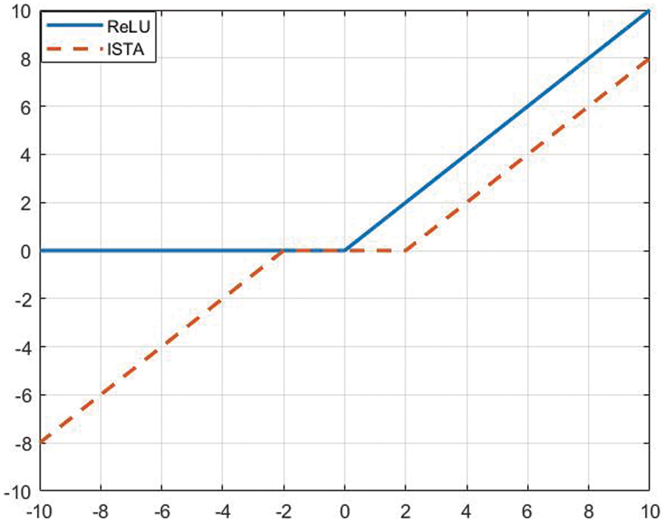
Figure 1: Sparse regularization strategy

The above discussion confines the problem to a single-layer model. The multiscale nature of DCNN is evident, formally defined as follows:

x=ReLU(ϕn⋯ReLU(ϕ2ReLU(ϕ1y+b1)+b2)+bn),n∈z.(9)

By extending the basic deep sparse representation to multiple layers, we can obtain the Multi-layer Deep Sparse Representation (ML-DSR) model, formally defined below:

x=D1α1α1=D2α2⋯αi−1=Diαi.(10)

this indicates that deep sparse representation also has a multi-scale analysis mechanism.

DCNN and sparse representation share similarities in optimization and feedback mechanisms. In DCNN, backpropagation is applied in each iteration to update the network parameters with respect to the loss function, using the gradient descent method. Such optimization and feedback mechanisms ensure that the final solution moves towards minimizing the error. In sparse representation, the dictionary is updated based on the feedback from the reconstruction error, and the update direction is towards minimizing the loss. This optimization mechanism is evident in convolutional sparse models, improving the learnability of dictionaries and network parameters.

3.2 High-Fidelity Reconstruction

Starting from the basic form of deep sparse representation X=Dα, assuming X={x1,x2,…, xn−1,xn}T and α={α1,α2,…,αn−1,αn}T, to achieve the reconstruction of the true value X, we need to pursue argmin ‖xi−Dαi‖22, where i=1⋯n, to obtain the optimal sparse coefficient α. Reference [10] provided the conditions for stable recovery of the original signal in the worst-case scenario. As follows:

||α||0≤14(1+1μ(D)),(11)

μ(D) represents the coherence of the dictionary D, which is defined by the maximum inner product of different atoms in the dictionary. The solution obtained by applying the pursuit algorithm to this is stable and reliable, satisfying the condition.

||α^−α||2≤4ε21−μ(D)(4||α||0−1),(12)

the symbol ε represents bounded noise disturbance to the signal, which indicates that perfect signal reconstruction can be achieved when ‖α^−α‖2, thereby achieving high-fidelity reconstruction. However, the precise pursuit of the sparse coefficient α is very difficult, so we relax the constraint on ‖α^−α‖2, and achieve a high-fidelity representation of the image under the condition that δ=‖α^−α‖2<σ.

Based on the Deep K-SVD algorithm, we constructed an artificial image dataset to validate its ability to effectively represent images through deep sparse representation, as shown in Fig. 2. The root mean square error (RMSE) was used to measure the error δ of the reconstructed artificial images. Fig. 3 shows the results of several artificial images reconstructed using deep sparse representation, which met our theoretical expectations in terms of visual effects and metrics analysis. The RMSE errors of the four test images reconstructed were 0.0185, 0.0667, 0.0326, and 0.0108, respectively, and the errors were within an acceptable range. This indicates that deep sparse representation can achieve the precise reconstruction of biological slice images, which establishes the basis for high-fidelity image inpainting.

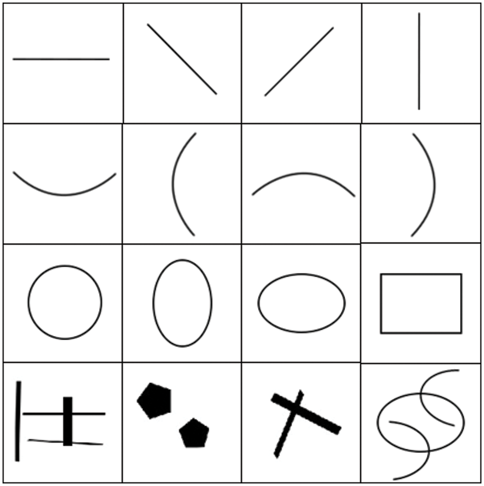
Figure 2: Artificial image datasets

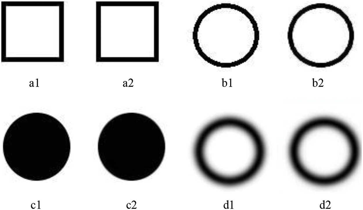
Figure 3: The reconstructed results of the test images. a1, b1, c1, and d1 are the original artificial images, while a2, b2, c2, and d2 are the reconstructed results

4  Deep Sparse Representation Inpainting

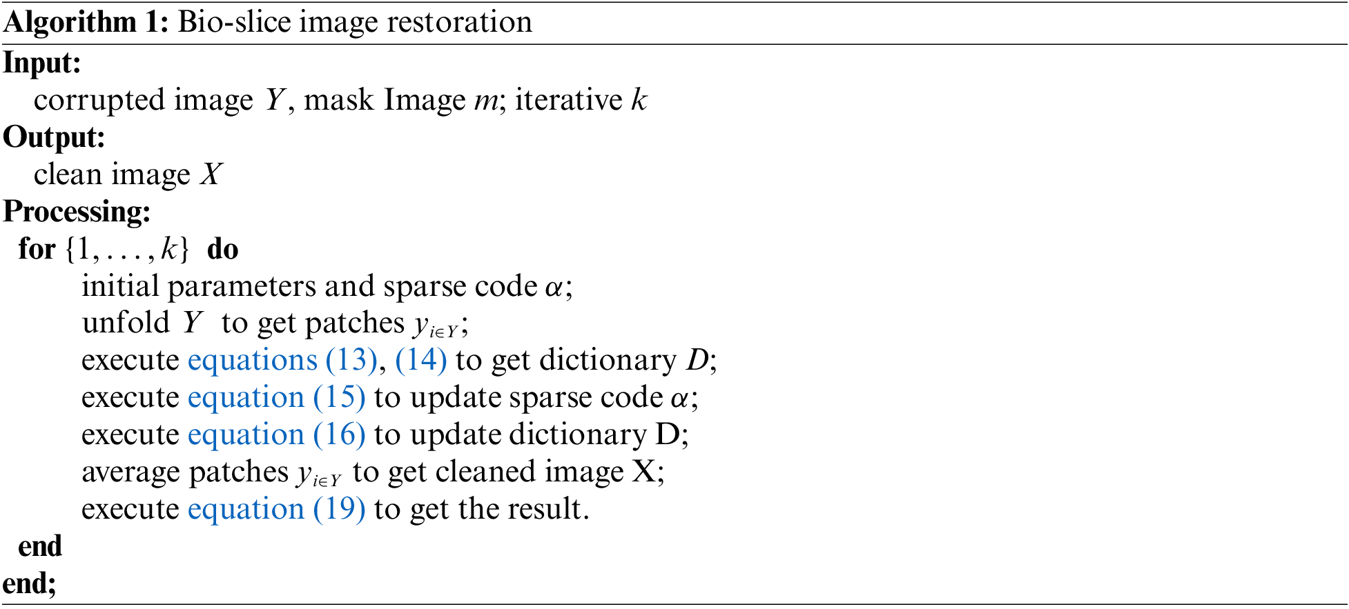
Our end-to-end biological slice image inpainting model is shown in Fig. 4. First, we construct a deep wavelet dictionary (DWDict) for the image y. Next, we decompose y into a collection of overlapping image blocks and generate corresponding sparse code. We then iteratively update the dictionary and sparse code in k layers. Finally, we obtain the reconstruction result by simple averaging. The error between the reconstruction result and the ground truth is fed back to the model to update the network’s parameters. Next, we will explain the details of dictionary construction and sparse coding.

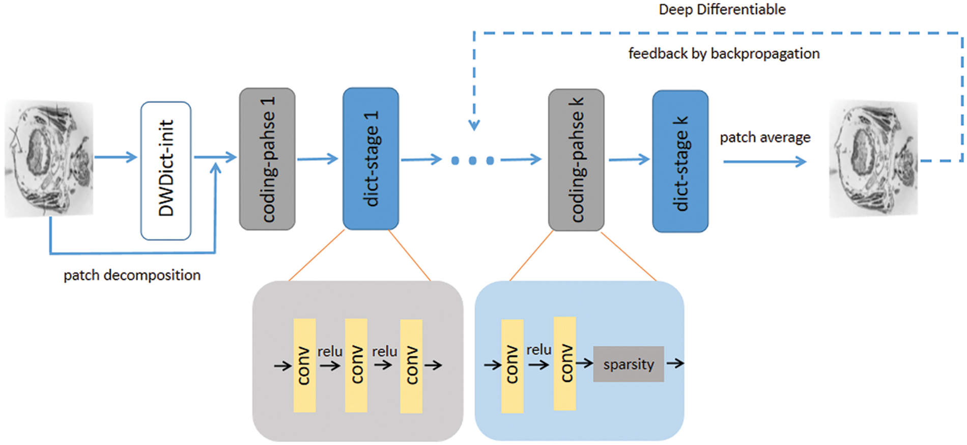
Figure 4: The algorithm architecture. The upper part represents the process of reconstructing damaged images, while the lower part shows the details of the encoding stage and dictionary update stage

4.1 Deep Wavelet Dictionary

Multiscale geometric analysis tools can achieve sparse representation of target images [31]. Using wavelet transform to construct a wavelet dictionary can further exploit the sparsity performance of the algorithm, and the prior knowledge obtained from the images can enhance the performance of deep learning algorithms [32]. However, wavelet transform basis functions rely on laborious designs, obtaining the optimal sparse representation of signal sets difficult. Therefore, we designed learnable wavelet basis functions and used the image prior knowledge to construct a Deep Wavelet Dictionary (DWDict), as shown in Fig. 5.

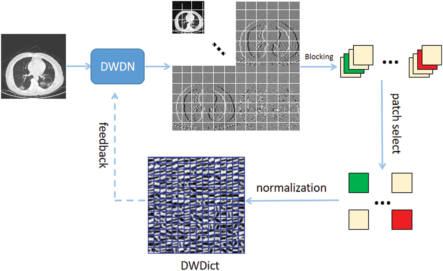
Figure 5: Algorithm flow for the construction of the deep wavelet dictionary

To meet the multiscale characteristics of wavelet decomposition, we first construct 2D discrete wavelet filters based on Eq. (5) and then construct a cascaded deep wavelet network as the convolutional kernel function to achieve convolutional operation and parameter learnability. Meanwhile, the down-sampling operation with a step size of 2 is performed to meet the requirements of each layer decomposition in the Fast Mallat algorithm. The form of the deep wavelet decomposition network is shown in Fig. 6. Let ℱi(n) be the non-linear function of the convolutional kernel function, and for signal S(t), the response of the deep wavelet decomposition network is shown in Eq. (13):

αi=<S(t),ψj,k(t)>=[S(t)ℱi(n)] ↓2,(13)

where ↓2 represents the down-sampling operator in the equation.

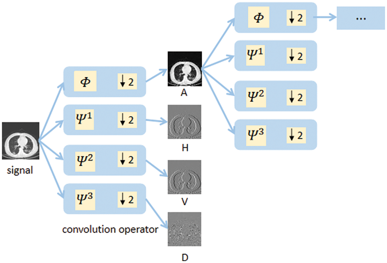
Figure 6: Deep wavelet decomposition network

The image Y is decomposed into a coefficient set α={αi|i=1,…,n} by the deep wavelet decomposition network, and we decompose the coefficient set α into a normalized coefficient block collection {Pk}k∈Iα according to the step size p and specification s. The coefficient block retains local information such as the edges of the image.

The dictionary should cover the entire space of x in space RN as much as possible. Does the K-SVD algorithm tend to learn what kind of atoms and does it meet the above ideas? We constructed some artificial images and used the K-SVD algorithm to generate their dictionaries, as shown in Fig. 7.

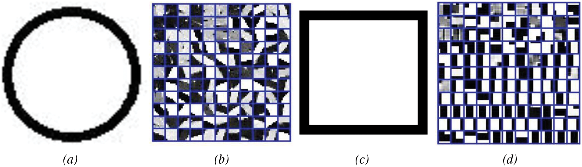
Figure 7: The results of K-SVD dictionary learning: (a) ring, (b) dictionary; (c) square, (d) dictionary

The K-SVD algorithm tends to favor learning the parts of the image with obvious features and selects representative parts from many feature areas as atoms. Based on this characteristic, we decided to prioritize image blocks with clear edge texture features in the construction of the deep wavelet dictionary. Therefore, we use the mean gradient as a measuring factor, which can characterize the degree of grayscale change, to select potential image blocks. The formula is defined as follows:

AG(P)=1MN∑iM⁡∑jN⁡(∂P∂x)2+(∂P∂y)22,(14)

in the formula, P represents the decomposed small blocks. To avoid the disturbance caused by the damaged areas on the dictionary construction, the image blocks in these areas will be excluded in advance.

4.2 Sparse Coding

Our sparsification strategy is to use a learnable ISTA algorithm to achieve sparse coding. The parameters of the ISTA algorithm rely entirely on manual design, which makes it difficult to achieve optimal sparse representation, especially for ill-posed inverse problems. To address this issue, Gregor et al. [33] proposed the Learned-ISTA algorithm to learn the model’s parameters, but its adaptability is not strong.

Due to the powerful representation capability of DCNN, the ISTA-Net algorithm [34] showed that nonlinear transformation functions can achieve sparse representation of images. The F(⋅)  operator constructed using nonlinear operators and ReLU linear units can achieve a richer expression of images. We use the learnability and nonlinearity of the F(⋅) operator to improve the sparsification performance of the sparse coding algorithm. Sparse coefficient α gets by α=F(α), and then as input to Eq. (15).

αk=sign(αk−1)ReLU(|αk−1|−ρ),k∈Z,(15)

in the equation, ρ=λ/L is a learnable parameter and its value is obtained by the MLP module to satisfy an appropriate stopping criterion for each small block.

ML-DSR shows that D or α can be a component of a layer, or can be used as the target signal. Therefore, we use the dictionary D as the target signal and deploy a shallow deep neural network model based on ML-DSR, which is updated in each iteration as defined below:

D=ReLU(ϕ3ReLU(ϕ2ReLU(ϕ1D+b)+b)+b),(16)

the dictionary also uses a deep differentiable method to optimize it during model feedback.

4.3 General Structure

The issue of small-scale corruption can be described as y=A⊙x, where ⊙ represents the element-wise product and A represents the limited operator. When addressing the damage caused by the limited operator, a new optimization objective function is obtained as shown in Eq. (19).

argminD, z12||x−ADz||22+λ||z||1.(17)

In the Deep K-SVD algorithm, the ℓ2 norm is used to measure the error between the true value and the reconstructed result, i.e., loss=‖x−f(y)‖2. However, the ℓ2 norm alone does not necessarily produce good sparse solutions and may cause artifacts, ignoring the visual perception demands of the human eye. Therefore, according to the suggestion in reference [33], a mixed form of ms_ssim and ℓ1 loss is used as the loss function.

ℒmix=αℒms_sssim+(1−α)ℒℓ1.(18)

As it is a global reconstruction for images with small-scale damage, information loss in the non-damaged areas of the image is inevitable. Therefore, we adopt the complement operation on the reconstructed result X, which allows us to focus on the reconstruction of the damaged areas and obtain better reconstruction results. The complement operation is defined as follows:

X=Y+X(∼M),(19)

the symbol “∼” represents a negation operation on the mask M. Finally, we can get the following algorithm flow.

5  Experiment

5.1 Data Sets and Preparatory Work

We used the frozen slice method to prepare the biological slices and stained them with uranyl acetate and lead citrate. Then we obtained 90 to 100 micrographs of lust microscopic slices by photographing them with a microscope. Processing the slice image by image enhancement methods such as shading correction and cropping. The process of slice image acquisition is shown in Fig. 8, The final obtained lust slice images contain rich texture information, complex edge contour structures, and segmental smoothness. In some tissue slices, there are also self-similar fractal structures [35], which reflect the complexity of biological structures. Sliced image inpainting has the following challenges: first, sliced images have complex texture contour information and thus need to be restored realistically at the time of inpainting, second, the low amount of sliced image data, and third, the need to avoid application difficulties due to high time complexity.

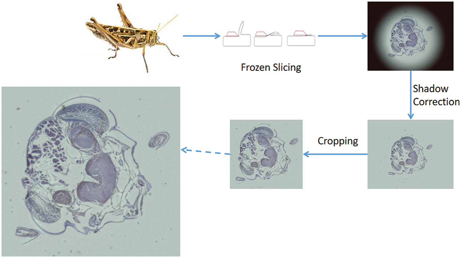
Figure 8: Biological sliced image preparation process

Due to the complexity of the slicing process and the small size of the data, we extract a specified number of images from the training set to effectively address the problem of insufficient data. Specifically, a m∗n sized image is cropped into (m−k+1)∗(n−k+1) sub-images of size k∗k. A manually crafted set of around 200 small-scale masks with different shapes are used to initialize the position of masks on the sliced images during data loading, to improve the generalization performance of the model.

Our model is built using the PyTorch framework and trained using the ADMM optimizer with a learning rate of 1e-4. The patch size is 8. The computer used for model training is equipped with an Intel(R) Xeon(R) Platinum 8255C CPU @ 2.50 GHz and NVIDIA GeForce RTX 3080. For model testing, both MATLAB R2021a and Python 3.7.4 environments were used on a computer with an Intel(R) Core(TM) i7-9750H CPU @ 2.60 GHz and NVIDIA GeForce GTX 1650.

5.2 Experiment Result

We design experiments from several aspects such as restoration effect, model complexity, and practicality, and use both simulated breakage and real breakage to show the restoration effect in the evaluation of inpainting effect. Fig. 9 shows the training loss, which was completed in just over 3 h. During testing and analysis, we used grayscale images of size 512 * 512 pixels for evaluation, including subjective and objective evaluations, time complexity comparison, model size comparison, and other assessment experiments that will be discussed in the following.

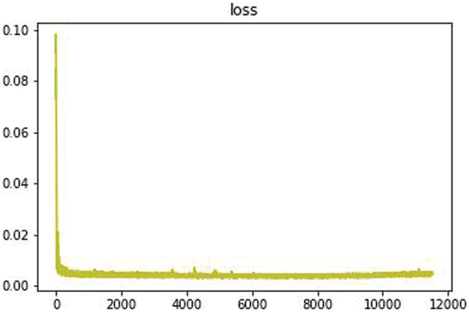
Figure 9: Training loss

As shown in Fig. 10, we constructed a DCT dictionary with 256 atoms and compared it to a deep wavelet dictionary with the same number of atoms. We found that the deep wavelet dictionary captures local feature information such as curved stripes, which are edge-like features, whereas the DCT dictionary mainly consists of striped and grid-like information. This indicates that the variety of atoms in the deep wavelet dictionary is more diverse, and the prior knowledge obtained from images can lead to better recovery performance of the algorithm.

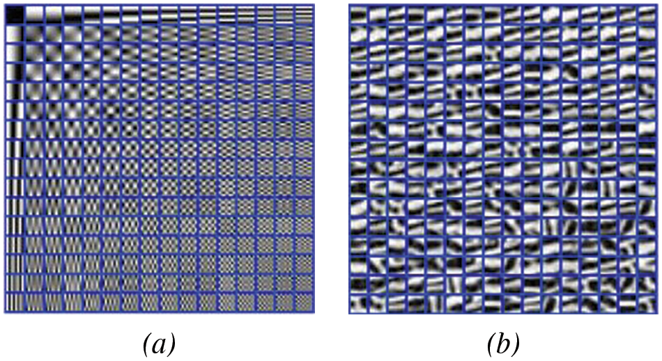
Figure 10: Dictionary construction algorithm, (a) is the DCT dictionary, (b) is the DWDict

To evaluate the effectiveness of our proposed algorithm, we compared it with classical image inpainting algorithms and deep learning-based image inpainting algorithms, including NLABH [36], Shearlet [37], Mumford-Shah [38], K-SVD [16], Deep Image Prior (DIP) [32], and Local Block Coordinate Descent Algorithm (LoBCoD) [39]. To assess the reconstruction quality of the algorithms, we used both subjective visual evaluation and objective evaluation metrics such as peak signal to noise ratio (PSNR), structural similarity index (SSIM), and root mean square error (RMSE), which can reflect the quality of image inpainting.

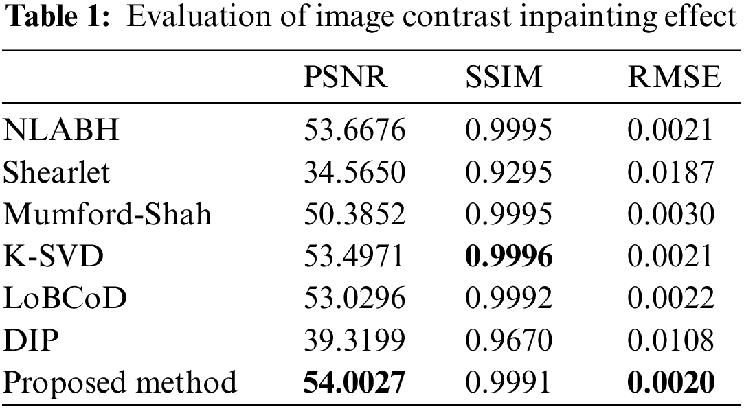
Fig. 11 shows the reconstruction results of different models after inpainting, and their evaluation metrics can be obtained from Table 1, which used simulated breakage masks. It can be observed that PDE-based inpainting methods such as Mumford-Shah algorithm exhibit strong competitiveness in small-scale damage inpainting by reasoning from the damaged edges towards the inside. LoBCoD algorithm, as a convolutional sparse coding model, uses the local block coordinate descent method to find the optimal basis vector and achieves good reconstruction performance. Compared with K-SVD algorithm, NLABH algorithm, our proposed algorithm achieves excellent subjective visual effects and optimal PSNR and RMSE scores, with SSIM score also approaching the optimal, reflecting the superior performance of our algorithm in reconstruction quality.

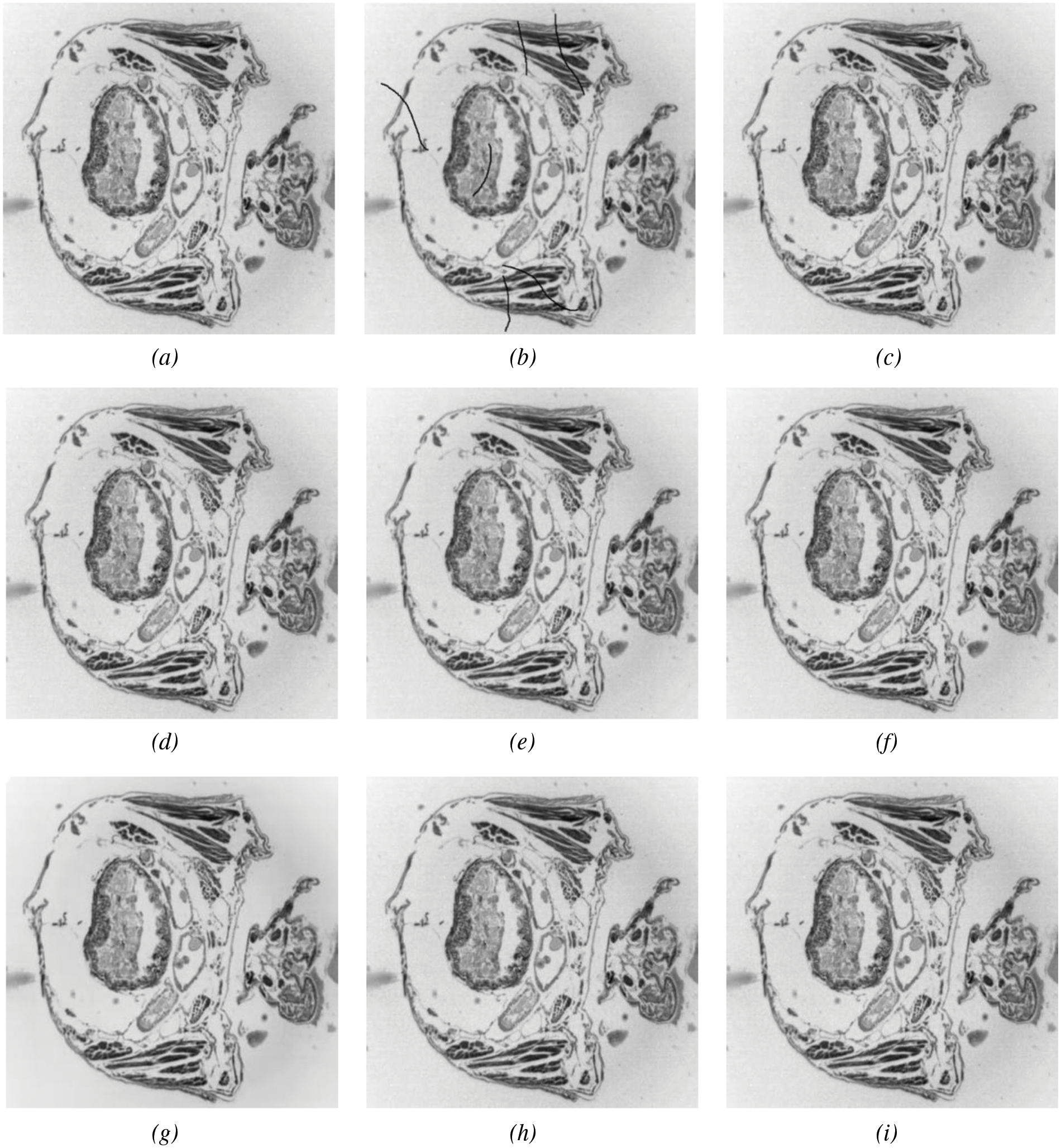
Figure 11: Slice image inpainting experiment: An original image, (b) masked image, (c) Mumford-Shah, (d) Shearlet, (e) NLABH, (f) K-SVDm, (g) DIP, (h) LoBCoD, and (i) Proposed algorithm

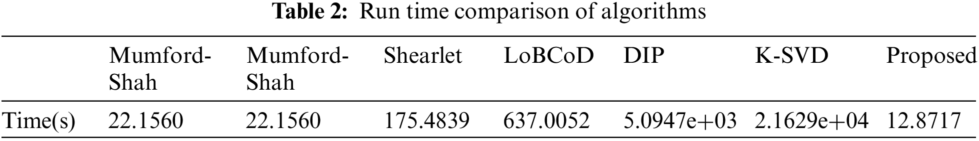
The time complexity of the algorithm is O(n2), which the bottleneck lies in the construction of the deep wavelet dictionary. Table 2 provides the running time of each model. We aim to evaluate the application value of the algorithms through a rough analysis of their running time. On the other hand, our proposed algorithm only takes less than 13 s to achieve comparable inpainting results to the K-SVD algorithm. Although the K-SVD algorithm also has good performance, its resource consumption is huge, reaching an intolerable time scale, making it difficult to apply in practical work. Table 2 and the reconstruction results discussed above demonstrate that our proposed algorithm not only achieves competitive inpainting results but also has practical application value. This is the goal we are pursuing.

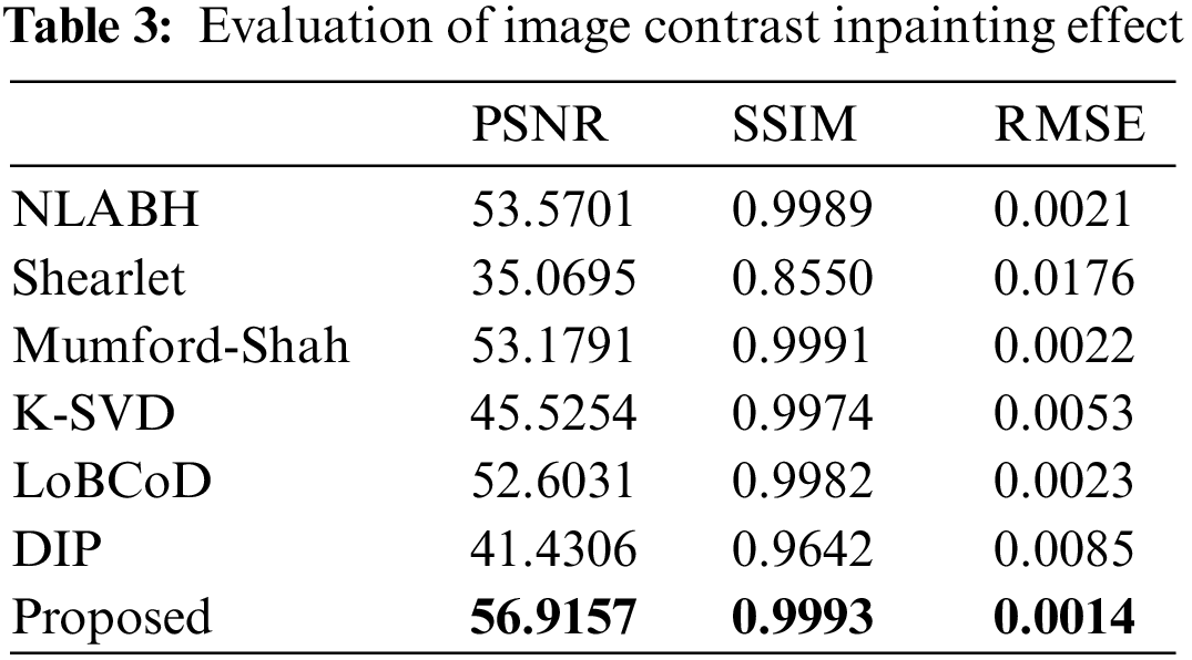
We conducted experimental comparisons on different forms of biological slice images to demonstrate the effectiveness of our proposed algorithm, as shown in Fig. 12 and Table 3. The highlighted red boxes demonstrate the rationality of our proposed algorithm in the inpainting of details. It can be seen that the PSNR indicator of the image after reconstruction using the multi-scale geometric analysis tool as a “sparse” expression tool is not ideal. This is because the geometric analysis tool adopts an approximation method, which brings information loss in the decomposition and reconstruction process. Compared to algorithms such as K-SVD and DIP, the algorithm proposed in this paper achieves a more natural and continuous transition at the boundaries of damaged regions. The SSIM value of the proposed algorithm reaches 0.993, which is an optimal result compared with other algorithms.

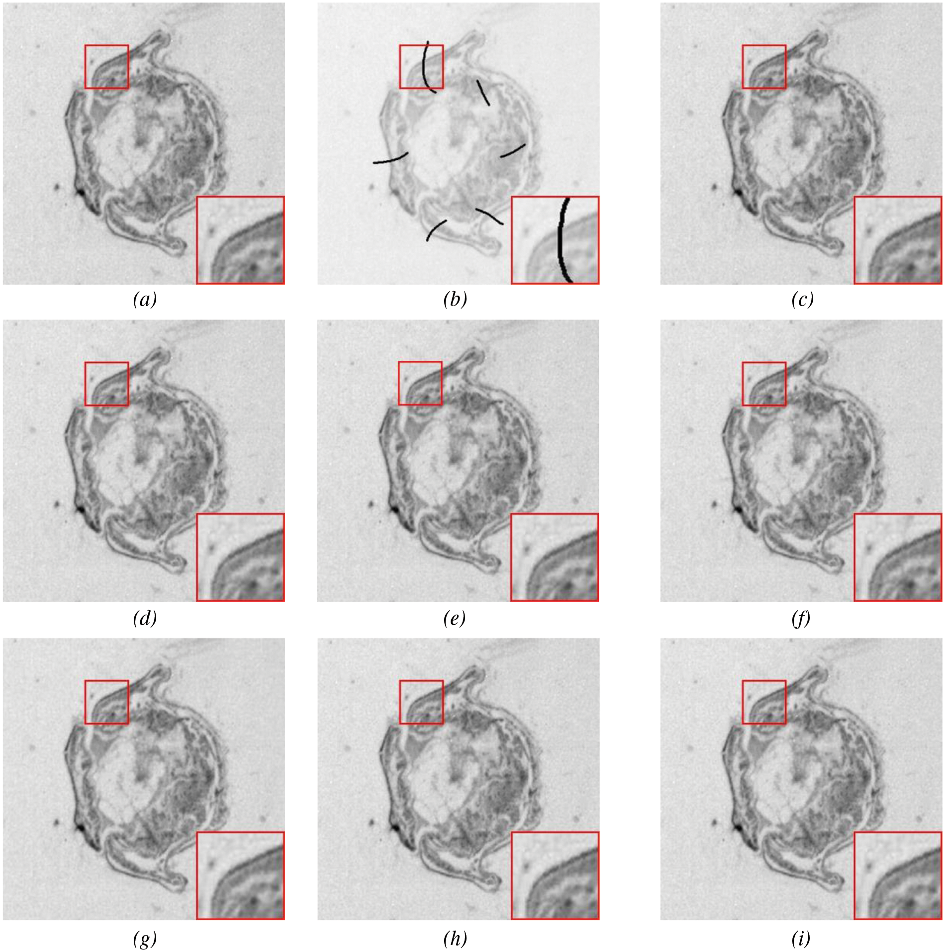
Figure 12: Slice image inpainting experiment: An original image, (b) masked image, (c) Mumford-Shah, (d) Shearlet, (e) NLABH, (f) K-SVDm, (g) DIP, (h) LoBCoD, and (i) Proposed algorithm

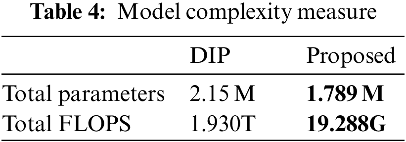
To further highlight the advantages of our proposed model in terms of small scale and low complexity, we used two indicators: the total number of parameters and the number of floating-point operations per second (FLOPS). The total number of parameters reflects the scale of the model, while FLOPS reflects the complexity of the model. As shown in Table 4, compared with the lightweight model of DIP, it can be seen that our proposed algorithm has a total number of parameters of only 1.789M, which is lower than the 2.15M of DIP. The GFLOPS indicator of our proposed model is 19.288G, much lower than the 1.930T of DIP. The significant difference in GFLOPS is that our proposed algorithm does not drastically increase in complexity with the scale of the problem.

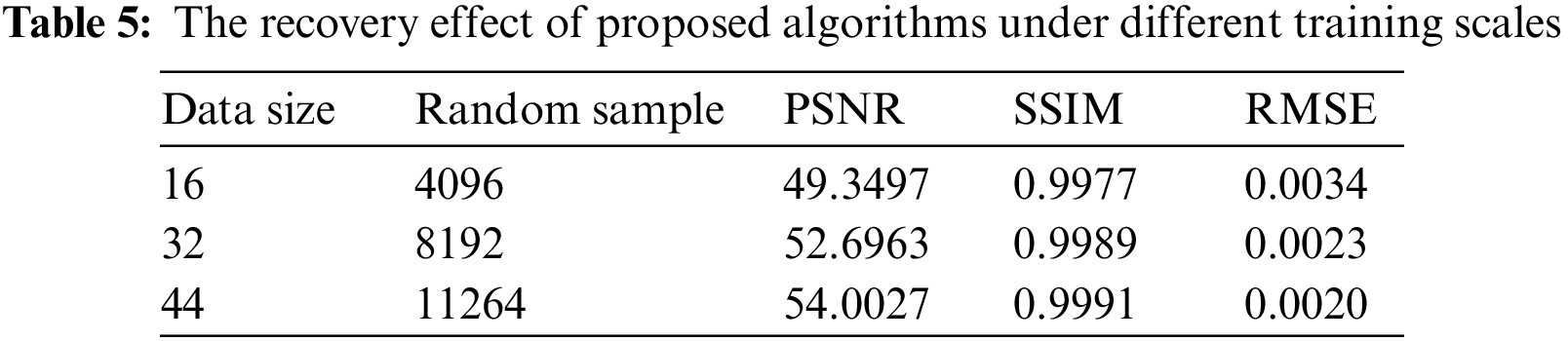
Another issue worth discussing is whether it is possible to train the model with fewer data to cope with the difficulty of acquiring images. As shown in Table 5, we trained the model with 16, 32, and 44 images, respectively, and evaluated the results. It can be seen that even with a small amount of data, the reconstructed results are acceptable, and the error level is kept below 0.004. This indicates that our proposed model has value in situations where data is difficult to obtain, and can adapt well to scenarios where it is hard to acquire biological image data.

Lastly, to demonstrate the practical application capability of the proposed algorithm in this paper, this chapter focuses on the application of the high-fidelity restoration algorithm to the problem of small-scale damages in biological slice images. As shown in Fig. 13, the location marked by the red box in the left image indicates the damaged area, which is labeled with a mask. It can be observed that the algorithm presented in this chapter achieves excellent restoration results for this real small-scale damage.

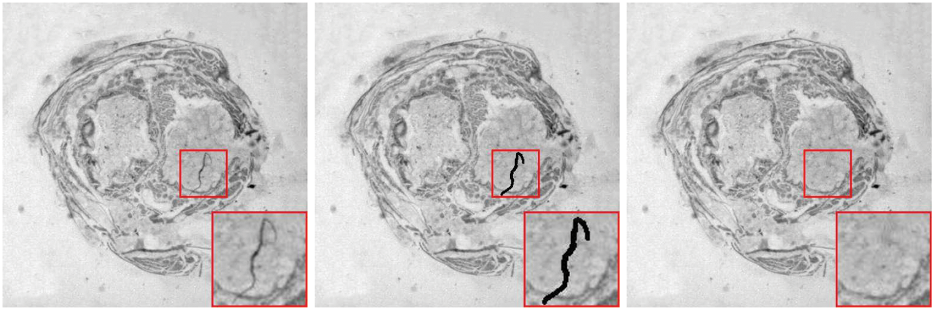
Figure 13: Realistic corruptions inpainting in slice images

6  Conclusion

This article focuses on the issue of small-scale corruption in biological slice image preparation, particularly in the case of limited data. We analyzed the relationship between sparse representation and deep neural networks and established a deep network model based on deep sparse representation. Our proposed model can effectively inpainting small-scale corruption in biological slice images while preserving the edge texture and contour structure of the slice images. We conducted tests using simulated damages, compared with other methods such as PDE-based methods, Shearlet algorithm, DIP algorithm, K-SVD algorithm, and sparse coding algorithm, our proposed model achieved good results in terms of effectiveness, time, and model scale. And then we demonstrated the application capability of our proposed method in addressing true corruptions in biological slice images that high-fidelity inpainting has been achieved.

Unlike algorithms such as K-SVD and LoBCOD, the algorithm proposed in this article not only achieves high-fidelity inpainting of biological slice images but also benefits from well-time complexity, making it valuable for practical applications. The proposed algorithm can also be effectively applied to other cross-sectional image restoration tasks, such as MRI and CT scan images. In future work, we will focus on explainable deep learning research based on deep sparse representation. Furthermore, the efficiency of the proposed model still needs further improvement, we will focus on dictionary learning with an emphasis on the learnable wavelet dictionary.

Acknowledgement: The authors extend their appreciation to the anonymous reviewers for their constructive comments and suggestions.

Funding Statement: This work was supported by the National Natural Science Foundation of China (Grant No. 61871380), the Shandong Provincial Natural Science Foundation (Grant No. ZR2020MF019), and Beijing Natural Science Foundation (Grant No. 4172034).

Author Contributions: Study conception and design: Haitao Hu, Shuli Mei; data collection: Haitao Hu, Hongmei Ma; analysis and interpretation of results: Haitao Hu, Shuli Mei, Hongmei Ma; draft manuscript preparation: Haitao Hu, Shuli Mei, Hongmei Ma. All authors reviewed the results and approved the final version of the manuscript.

Availability of Data and Materials: The data that support the findings of this study are available from the corresponding author upon reasonable request.

Conflicts of Interest: The authors declare that they have no conflicts of interest to report regarding the present study.

References

1. P. Herreros, S. Tapia-Gonzalez, L. Sanchez-Olivares, M. F. L. Heras and M. Holgado, “Alternative brain slice-on-a-chip for organotypic culture and effective fluorescence injection testing,” International Journal of Molecular Sciences, vol. 23, no. 5, pp. 2549, 2022. [Google Scholar] [PubMed]

2. H. Wang, J. Liu, L. Liu, M. Zhao and S. Mei, “Coupling technology of opensurf and shannon-cosine wavelet interpolation for locust slice images inpainting,” Computers and Electronics in Agriculture, vol. 198, pp. 107110, 2022. [Google Scholar]

3. L. Li, G. Shuangshuang, M. Shuli and Z. Nannan, “Image restoration of locust slices based on nearest unit matching,” Transactions of the Chinese Society of Agricultural Machinery, vol. 46, no. 8, pp. 15–19, 2015. [Google Scholar]

4. A. Criminisi, P. Perez and K. Toyama, “Region filling and object removal by exemplar-based image inpainting,” IEEE Transactions on Image Processing, vol. 13, no. 9, pp. 1200–1212, 2004. [Google Scholar] [PubMed]

5. D. Pathak, P. Krahenbuhl, J. Donahue, T. Darrell and A. A. Efros, “Context encoders: Feature learning by inpainting,” in 2016 IEEE Conf. on Computer Vision and Pattern Recognition (CVPR), Seattle, WA, USA, pp. 2536–2544, 2016. [Google Scholar]

6. H. Xiang, Q. Zou, M. A. Nawaz, X. Huang, F. Zhang et al., “Deep learning for image inpainting: A survey,” Pattern Recognition, vol. 134, pp. 109046, 2023. [Google Scholar]

7. K. Meng, M. Liu, S. Mei and L. Yang, “A high-fidelity inpainting method of micro-slice images based on bendlet analysis,” Biosystems Engineering, vol. 230, pp. 16–34, 2023. [Google Scholar]

8. D. L. Donoho, “Compressed sensing,” IEEE Transactions on Information Theory, vol. 52, no. 4, pp. 1289–1306, 2006. [Google Scholar]

9. E. J. Candes, J. Romberg and T. Tao, “Robust uncertainty principles: Exact signal reconstruction from highly incomplete frequency information,” IEEE Transactions on Information Theory, vol. 52, no. 2, pp. 489–509, 2006. [Google Scholar]

10. R. Khatib, D. Simon and M. Elad, “Learned greedy method (LGMA novel neural architecture for sparse coding and beyond,” Journal of Visual Communication and Image Representation, vol. 77, pp. 103095, 2021. [Google Scholar]

11. V. Papyan, Y. Romano, J. Sulam and M. Elad, “Theoretical foundations of deep learning via sparse representations a multilayer sparse model and its connection to convolutional neural networks,” IEEE Signal Processing Magazine, vol. 35, no. 4, pp. 72–89, 2018. [Google Scholar]

12. V. Papyan, Y. Romano and M. Elad, “Convolutional neural networks analyzed via convolutional sparse coding,” Journal of Machine Learning Research, vol. 18, no. 83, pp. 1–52, 2017. [Google Scholar]

13. R. Rubinstein, A. M. Bruckstein and M. Elad, “Dictionaries for sparse representation modeling,” Proceedings of the IEEE, vol. 98, no. 6, pp. 1045–1057, 2010. [Google Scholar]

14. Q. Lian, B. Shi and S. Chen, “Research advances on dictionary learning models, algorithms and applications,” Acta Automatica Sinica, vol. 41, no. 2, pp. 240–260, 2015. [Google Scholar]

15. Z. Huang, Z. Wang, Q. Li, J. Chen, Y. Zhang et al., “DSRD: Deep sparse representation with learnable dictionary for remotely sensed image denoising,” International Journal of Remote Sensing, vol. 43, no. 7, pp. 2699–2711, 2022. [Google Scholar]

16. M. Aharon, M. Elad and A. Bruckstein, “K-SVD: An algorithm for designing overcomplete dictionaries for sparse representation,” IEEE Transactions on Signal Processing, vol. 54, no. 11, pp. 4311–4322, 2006. [Google Scholar]

17. D. Yang and J. Sun, “BM3D-Net: A convolutional neural network for transform-domain collaborative filtering,” IEEE Signal Processing Letters, vol. 25, no. 1, pp. 55–59, 2018. [Google Scholar]

18. K. Zhang, W. Zuo, Y. Chen, D. Meng and L. Zhang, “Beyond a Gaussian denoiser: Residual learning of deep CNN for image denoising,” IEEE Transactions on Image Processing, vol. 26, no. 7, pp. 3142–3155, 2017. [Google Scholar] [PubMed]

19. M. Scetbon, M. Elad and P. Milanfar, “Deep K-SVD denoising,” IEEE Transactions on Image Processing, vol. 30, pp. 5944–5955, 2021. [Google Scholar] [PubMed]

20. M. Abavisani and V. M. Patel, “Deep multimodal sparse representation-based classification,” in 2020 IEEE Int. Conf. on Image Processing (ICIP), Abu Dhabi, United Arab Emirates, pp. 773–777, 2020. [Google Scholar]

21. G. Michau, G. Frusque and O. Fink, “Fully learnable deep wavelet transform for unsupervised monitoring of high-frequency time series,” Proceedings of the National Academy of Sciences of the United States of America, vol. 119, no. 8, pp. e2106598119, 2022. [Google Scholar] [PubMed]

22. S. G. Mallat, “A theory for multiresolution signal decomposition—The wavelet representation,” IEEE Transactions on Pattern Analysis and Machine Intelligence, vol. 11, no. 7, pp. 674–693, 1989. [Google Scholar]

23. S. Herbreteau and C. Kervrann, “DCT2net: An interpretable shallow cnn for image denoising,” IEEE Transactions on Image Processing, vol. 31, pp. 4292–4305, 2022. [Google Scholar] [PubMed]

24. A. Singh, K. Raj, T. Kumar, S. Verma and A. M. Roy, “Deep learning-based cost-effective and responsive robot for autism treatment,” Drones, vol. 7, no. 2, pp. 81, 2023. [Google Scholar]

25. A. K. Saydjari and D. P. Finkbeiner, “Equivariant wavelets: Fast rotation and translation invariant wavelet scattering transforms,” IEEE Transactions on Pattern Analysis and Machine Intelligence, vol. 45, no. 2, pp. 1716–1731, 2023. [Google Scholar] [PubMed]

26. W. Xu, Q. Zhu, N. Qi and D. Chen, “Deep sparse representation based image restoration with denoising prior,” IEEE Transactions on Circuits and Systems for Video Technology, vol. 32, no. 10, pp. 6530–6542, 2022. [Google Scholar]

27. M. Abavisani and V. M. Patel, “Deep sparse representation-based classification,” IEEE Signal Processing Letters, vol. 26, no. 6, pp. 948–952, 2019. [Google Scholar]

28. Y. Li, C. Chen, F. Yang and J. Huang, “Deep sparse representation for robust image registration,” in 2015 IEEE Conf. on Computer Vision and Pattern Recognition (CVPR), Boston, MA, USA, pp. 4894–4901, 2015. [Google Scholar]

29. X. Glorot, A. Bordes and Y. Bengio, “Deep sparse rectifier neural networks,” Journal of Machine Learning Research, vol. 15, pp. 315–323, 2011. [Google Scholar]

30. I. Daubechies, M. Defrise and C. de Mol, “An iterative thresholding algorithm for linear inverse problems with a sparsity constraint,” Communications on Pure and Applied Mathematics, vol. 57, no. 11, pp. 1413–1457, 2004. [Google Scholar]

31. B. Ophir, M. Lustig and M. Elad, “Multi-scale dictionary learning using wavelets,” IEEE Journal of Selected Topics in Signal Processing, vol. 5, no. 5, pp. 1014–1024, 2011. [Google Scholar]

32. D. Ulyanov, A. Vedaldi and V. Lempitsky, “Deep image prior,” in 2018 IEEE/CVF Conf. on Computer Vision and Pattern Recognition (CVPR), Salt Lake City, UT, USA, pp. 9446–9454, 2018. [Google Scholar]

33. K. Gregor and Y. Lecun, “Learning fast approximations of sparse coding,” in Proc. of the 27th Int. Conf. on Machine Learning, Omnipress, Haifa, Israel, pp. 399–406, 2010. [Google Scholar]

34. J. Zhang and B. Ghanem, “ISTA-Net: Interpretable optimization-inspired deep network for image compressive sensing,” in 2018 IEEE/CVF Conf. on Computer Vision and Pattern Recognition (CVPR), Salt Lake City, UT, USA, pp. 1828–1837, 2018. [Google Scholar]

35. H. Wang, X. Zhang and S. Mei, “Shannon-cosine wavelet precise integration method for locust slice image mixed denoising,” Mathematical Problems in Engineering, vol. 2020, pp. 1–17, 2020. [Google Scholar]

36. Y. Wen, L. A. Vese, K. Shi, Z. Guo and J. Sun, “Nonlocal adaptive biharmonic regularizer for image restoration,” Journal of Mathematical Imaging and Vision, vol. 65, no. 3, pp. 453–471, 2023. [Google Scholar]

37. G. Kutyniok, W. Lim and R. Reisenhofer, “Shearlab 3D: Faithful digital shearlet transforms based on compactly supported shearlets,” Acm Transactions on Mathematical Software, vol. 42, no. 5, pp. 1–42, 2016. [Google Scholar]

38. Z. Xu, X. Lian and L. Feng, “Image inpainting algorithm based on partial differential equation,” in 2008 ISECS Int. Colloquium on Computing, Communication, Control, and Management, Guangzhou, China, pp. 120–124, 2008. [Google Scholar]

39. E. Zisselman, J. Sulam and M. Elad, “A local block coordinate descent algorithm for the csc model,” in 2019 IEEE/CVF Conf. on Computer Vision and Pattern Recognition (CVPR 2019), Long Beach, CA, USA, pp. 8200–8209, 2019. [Google Scholar]