
 Submit a Paper
 Propose a Special lssue
 Open Access
ARTICLE
Micro-Expression Recognition Based on Spatio-Temporal Feature Extraction of Key Regions
1 College of Computer Science, Hunan University of Technology, Zhuzhou, 412007, China
2 Intelligent Information Perception and Processing Technology, Hunan Province Key Laboratory, Zhuzhou, 412007, China
* Corresponding Author: Qiang Liu. Email:
Computers, Materials & Continua 2023, 77(1), 1373-1392. https://doi.org/10.32604/cmc.2023.037216
Received 27 October 2022; Accepted 03 March 2023; Issue published 31 October 2023
 View Full Text
 Download PDF
Abstract
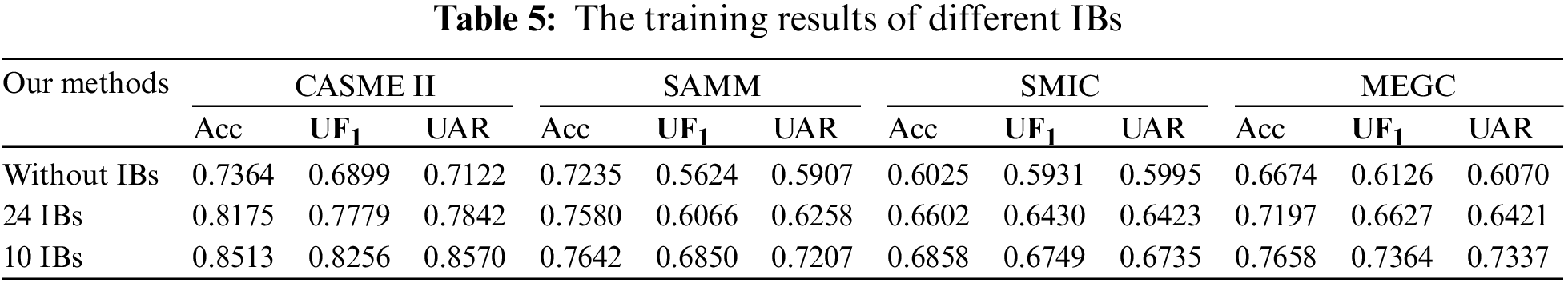
Aiming at the problems of short duration, low intensity, and difficult detection of micro-expressions (MEs), the global and local features of ME video frames are extracted by combining spatial feature extraction and temporal feature extraction. Based on traditional convolution neural network (CNN) and long short-term memory (LSTM), a recognition method combining global identification attention network (GIA), block identification attention network (BIA) and bi-directional long short-term memory (Bi-LSTM) is proposed. In the BIA, the ME video frame will be cropped, and the training will be carried out by cropping into 24 identification blocks (IBs), 10 IBs and uncropped IBs. To alleviate the overfitting problem in training, we first extract the basic features of the pre-processed sequence through the transfer learning layer, and then extract the global and local spatial features of the output data through the GIA layer and the BIA layer, respectively. In the BIA layer, the input data will be cropped into local feature vectors with attention weights to extract the local features of the ME frames; in the GIA layer, the global features of the ME frames will be extracted. Finally, after fusing the global and local feature vectors, the ME time-series information is extracted by Bi-LSTM. The experimental results show that using IBs can significantly improve the model's ability to extract subtle facial features, and the model works best when 10 IBs are used.Keywords
Compared with traditional expressions, MEs are expressions of short duration and small movements. As a spontaneous expression, ME is produced when people try to cover up their genuine internal emotions. It is an expression that can neither be forged nor suppressed [1]. In 1966, Haggard et al. [2] discovered a facial expression that is fast and not easily detected by the human eye and first proposed the concept of MEs. At first, this small and transient facial change did not attract the attention of other peer researchers. Until 1969, when Ekman et al. [3] studied a video of depression, he found that patients with smiling expressions would have extremely brief painful expressions. The patient tried to hide his anxiety with a more positive expression, such as a smile. Unlike macro-expressions, MEs only last for 1/25~1/5 second. Therefore, recognition only by human eyes does not meet the need for accurate identification [4,5], and it is essential to use modern artificial intelligence means.
Research on micro-expression recognition (MER) has undergone a shift from using traditional image feature extraction methods to deep learning feature extraction methods. Pfister et al. [6,7] extended the feature extraction method from XY direction to three orthogonal planes composed of XY, XT and YT by using the local binary patterns from three orthogonal planes (LBP-TOP) algorithm. The LBP-TOP algorithm has been extended from the previous static feature extraction to the dynamic feature extraction that changes with time information. But this recognition method is not ideal for MEs with small intensity changes. Xia et al. [8] found the problem that facial details with minor changes in MER can quickly disappear in deep models. He demonstrated that lower resolution input data and shallower model structure could help alleviate the phenomenon of detail disappearance. Then, he further proposed a recurrent convolutional network (RCN) to reduce the model and data. However, compared to the CNN with attention mechanisms, this design does not perform well in deep models. Xie et al. [9] proposed an MER method based on action units (AUs). Based on the correlation between facial muscles and AUs, this method improves the recognition rate of MEs to a certain extent. Li et al. [10] proposed a model structure based on 3DCNN, an MER method combining attention mechanism and feature fusion. This model extracts optical flow features and facial features through a deep CNN and adds transfer learning to alleviate the problem of model overfitting. Gan et al. [11] proposed the OFF-ApexNet framework by using the optical flow characteristics between images, which can input the extracted optical flow characteristics between onset frame, apex frame and offset frame into CNN for recognition. However, the ME change is a continuous process, and only relying on the onset frame, apex frame and offset frame may ignore the details between video sequences. Huang et al. [12] proposed a method of MER by using the optical flow characteristics of apex frames and integrating the SHCFNet framework. The SHCFNet framework combines the extraction of spatial and temporal features, but it ignores the processing of local detail features of MEs. Zhan et al. [13] proposed an MER method based on an evolutionary algorithm and named it the GP (genetic programming) algorithm. The GP algorithm can select representative sequence frames from ME video frames and guide individuals to evolve toward higher recognition ability. This method can efficiently extract time-varying sequence features in MER. But it only performs feature extraction globally and does not consider that the importance of different parts of the face varies in MER. Tang et al. [14] proposed a model based on the optical flow method and Pseudo 3D Residual Network (P3D ResNet). This method uses the optical flow method to extract the characteristic information of the ME optical flow sequence, then extracts the spatial information and temporal information of the ME sequence through the P3D ResNet model, and finally classifies and outputs it. However, P3D ResNet is more based on the entire area of the face and does not take into account the minor detail changes in the local MEs. Niu et al. [15] proposed a CBAM-DPN algorithm based on a convolutional attention module and a dual-channel network. The method fuses channel attention and spatial attention, thus enabling feature extraction of local details of MEs. Simultaneously, the DPN structure can inhibit useless features and enhance the expression ability of model features. But this method only relies on apex frames, ignoring the sequence correlation between ME video frames.
To solve the problems of low intensity, short duration and difficult detection of ME, we propose a method for MER using key facial regions. This method can extract spatial and temporal information from ME frames. The design of the local IBs in the experiments overcomes the shortcoming of only utilizing global feature extraction in the SHCFNet [12] framework. Compared with the OFF-ApexNet [11] framework, our method utilizes all video frames from onset to apex, which can further extract more detailed facial change information. After the spatial feature extraction, we added the Bi-LSTM framework, which can further extract the sequence features of the video frames compared with the CBAM-DPN [15,16] algorithm, thereby improving the recognition accuracy. In addition, to further extract the facial details of MEs, in the experiment, we crop the ME video frames into IBs and perform ablation experiments on the uncropped IBs, 24 and 10 IBs. Finally, according to the experimental results, the selected schemes of different IBs are compared.
2.1 Facial Expression Coding System (FACS)
There are 42 muscles in the human face. The rich expression changes are the result of the joint action of a variety of muscles. Some facial muscles that can be consciously controlled are called “voluntary muscles”. There are also some facial muscles that can not be under conscious control are called “involuntary muscles”. In 1976, Ekman et al. [3] proposed a facial expression coding system (FACS) based on facial anatomy. FACS divides the human face into 44 AUs. Different AUs represent different local facial actions. For example, AU1 represents the inner browser raiser, while AU5 represents the upper lip raiser [17–19]. ME generation is usually the result of the joint action of one or more AUs. For example, the ME representing happiness results from the joint action of AU6 and AU12, where AU16 represents the downward pull of the lower lip and AU12 represents the upward corner of the mouth. FACS is an essential basis for MER, and it also is an action record of facial key point features such as eyebrows, cheeks and corners of the mouth [20–22]. In our experiment, the face will be divided into several ME IBs according to the AU.
2.2 Neural Network with Attention Mechanism
To address the shortcomings of short duration and low action intensity in MER, we add an attention mechanism in a CNN [23]. This design makes the CNN model not only extract the features of the whole face but also focus on the changes in local details. It enables the model to extract more subtle facial detail features in MER. CNN can extract the abstract features of ME [24]. The CNN with a local attention network is used to extract the motion information of critical local units in ME change. In contrast, the CNN with a global attention network can extract the global change information. In the experiment, we combine the CNN with the local attention mechanism and the CNN with the global attention mechanism. We expect the improved CNN model to have the ability to pay attention to both the global and the details.
2.3 Bi-Directional Long Short-Term Memory Network (Bi-LSTM)
Traditional CNNs and fully connected (FC) layers have a common feature in that they cannot “memorize” relevant information between time series when dealing with continuous sequences [25]. Compared with traditional neural networks, recurrent neural network (RNN) adds a hidden layer that can save state information. This hidden layer includes historical information about the sequence and updates itself with the input sequence. However, the most significant disadvantage of traditional RNN is that with the increase of training scale and layers, it is easy to produce long-term dependencies problems [26,27]. That is, it is easy to produce gradient disappearance and gradient explosion when learning a long sequence. To solve the above problems of RNNs, in the early 1990s, Hochreiter et al. proposed LSTM. Each unit block of LSTM includes an input gate, forget gate and output gate [28]. The input gate is used to determine how much input data at the current time can be saved to the current state unit; The forgetting gate is used to indicate how many state units at the last time can be saved to this state unit; The output gate controls how many current state units can be used for output. Bi-LSTM adds a backpropagation layer to the LSTM which make the Bi-LSTM model can use not only historical sequence information but also future information [29]. Simultaneously, Bi-LSTM can better extract the feature and sequence information in ME than LSTM.
We propose a neural network structure based on the combination of CNN with attention mechanism and Bi-LSTM. To accurately capture small-scale facial movements, we add global and local attention mechanisms [30] to the traditional CNN framework. The improved framework can extract different feature information from multiple facial regions. Simultaneously, we also increase the processing of global information. The improved model architecture is shown in Fig. 1. Firstly, the network uses the transfer learning method to pass the pre-processed feature vector through the VGG16 model with pre-training weight and extract the basic facial features [31]. Then, the facial features extracted from each frame are passed through GIA and BIA to extract global and local information. Afterward, we fuse the extracted global and local information and extract the sequence-related information through Bi-LSTM. Finally, the classification output is carried out through a three-layer FC layer.
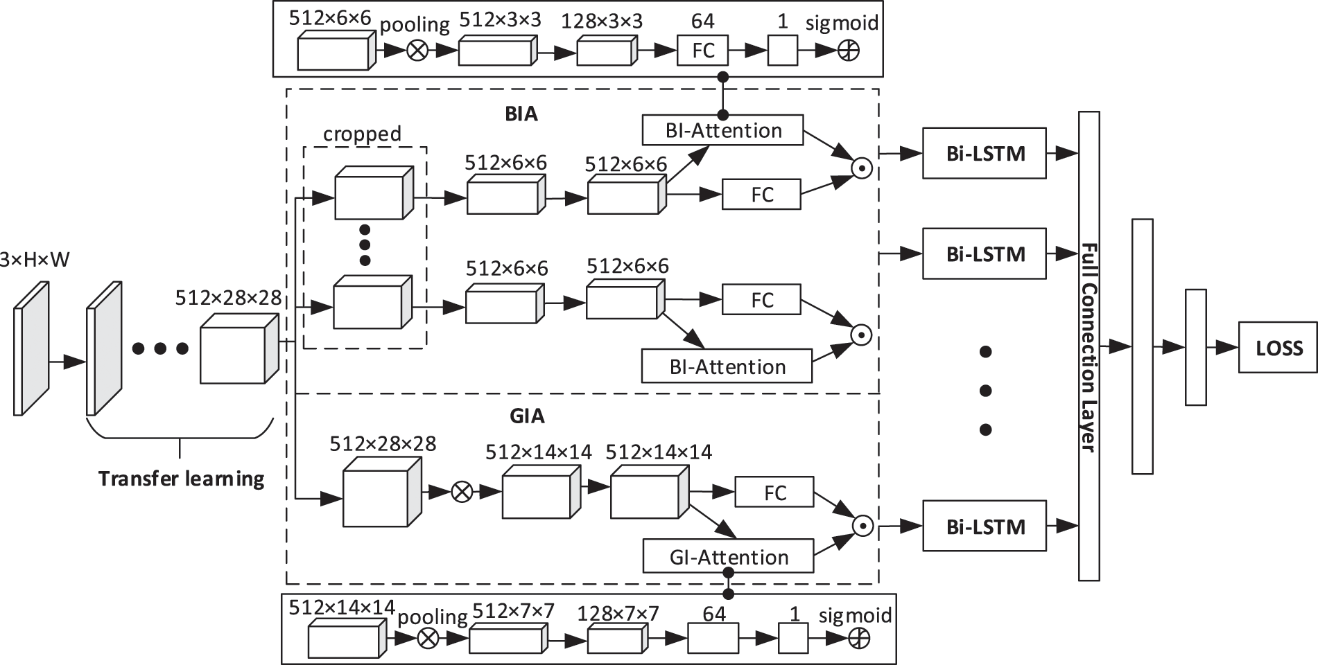
Figure 1: The model combining GIA, BIA and Bi-LSTM. It includes a transfer learning layer, GIA and BIA layer, Bi-LSTM layer and FC layer
To extract the global and local features of the face, we introduce the BIA and GIA frameworks. As shown in Fig. 1, BIA is the upper part of the dashed box in the figure, and GIA is the lower part of the dashed box in the figure.
The range of facial variation of ME is small, which is challenging to be recognized effectively. This experiment adopts the recognition method of increasing the blocks with attention in the critical regions of the face. The representative area and the corresponding attention weight are added to the facial features to be recognized. In the experiments, we will perform ablation experiments on uncropped, cropped into 24 and 10 ME blocks, respectively.
3.2.1 The Neural Network with Attention Mechanism
BIA is shown in the upper part of the dashed box in Fig. 1. After cropping in the BIA, the local IBs are obtained, and then each IB vector goes through an FC layer and an attention network whose output is a weighted scalar. Finally, each IB gets a weighted feature vector and outputs it.
In the attention network (the upper half of the dashed box in Fig. 1), it is assumed that
3.2.2 Generation Method of 24 IBs
To accurately recognize the local details of the face, we generate 24 detailed IBs based on facial key points. There are Dlib [32] method and face_recognition [33] method to determine face key points. The Dlib method can obtain 68 facial key points (see Fig. 2a), and the face_recognition method can obtain 72 facial key points (see Fig. 2b). In experiments, we found that the face_recognition method can obtain more accurate facial key point information than the Dlib method. Therefore, we use the face_recognition method to achieve precise positioning when determining the ME IB. The 24 IBs are generated as follows:
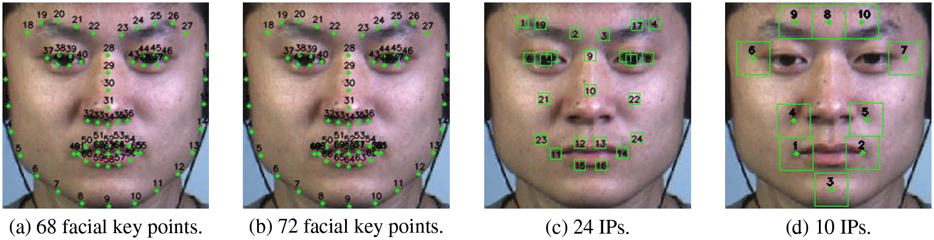
Figure 2: Comparison of ME key points and IPs. (a) 68 facial key points (b) 72 facial key points (c) 24 IPs (d) 10 IPs. We select 24 and 10 IPs for experiments on 72 facial key points, respectively
(1) Determine the identification points (IPs): We first extracted 72 facial key points using the face_recognition method (see Fig. 2b). Then, based on 72 facial key points, We converted them to 24 IPs. The location of IPs covers the cheeks, mouth, nose, eyes and eyebrows. The conversion process is as follows. Firstly, 16 IPs covering mouth, nose, eyes and eyebrows are selected from 72 facial key points. The extraction sequence numbers of 72 facial key points (see Fig. 2b) are: 19, 22, 23, 26, 39, 37, 44, 46, 28, 30, 49, 51, 53, 55, 59 and 57. The serial numbers of the IPs generated (see Fig. 2C) are: 1, 2, 3, 4, 5, 6, 7, 8, 9, 10, 11, 12, 13, 14, 15 and 16. Secondly, for the eyes, eyebrows and cheeks, we generate them through the midpoint coordinates of the key points. For the left eye, left eyebrow and left cheek, we select the midpoint coordinates of (20, 38), (41, 42), (18, 59) point pairs from 72 facial key points (see Fig. 2b) as the IPs; For the right eye, right eyebrow and right cheek, we select the midpoint coordinates of (25, 45), (47, 48) and (27, 57) point pairs from 72 facial key points as the IPs; The serial numbers of the generated IPs (see Fig. 2c) are: 17, 19, 18, 20, 21 and 22. Finally, for the left and right corners of the mouth, we select 49 and 55 keys from 72 facial keys (see Fig. 2b). Then, according to the coordinates of the two points, the relative offset points of the two corners of the mouth are selected as the generation basis of the coordinates of the IPs. The generated IPs at the left and right corners of the mouth (see Fig. 2C) are numbered 23 and 24. Eqs. (4) and (5) are the calculation methods of the IPs at the left and right corners of the mouth. Wherein
(2) Generate IBs: Finally, we got 24 IPs (see Fig. 2c). The re-selected 24 IPs will generate 24 48 × 48 IBs centered on the IPs. To improve the robustness of the model, we perform feature extraction on IBs after passing through the transfer learning layer.
3.2.3 Generation Method of 10 IBs
The 24 IBs can cover the face area relatively wholly, but in the experiment we found that covering the face area too finely may make BIA learn some redundant features. In subsequent experiments, we obtained 10 IBs based on FACS. The 10 IBs relatively completely covered the eyebrows, eyes, nose, mouth and chin of the human face. The detailed experimental steps for obtaining 10 IBs are as follows:
(1) Determine the IPs: we obtained 72 facial key points through face_recognition and then converted them into 10 IPs. The conversion process is as follows: we first determine the side length of the IB area. We selected half of the abscissa distance between points 49 and 55 (see Fig. 2b) as the side length of the IB area. For the eyebrow part, we select the midpoint coordinates of the 20th and 25th points (see Fig. 2b) among the 72 facial key points as the coordinates of the 8th IP (see Fig. 2d). The 9th and 10th IPs are generated based on the existing 8th IP. The generation method of the 9th and 10th IPs is shown in Eqs. (6) and (7). Where
For the eyes, we select the coordinates of the 37th and 46th points (see Fig. 2b) among the 72 facial key points as the coordinate generation basis of the 6th and 7th IPs (see Fig. 2d). The generation method of IPs 6 and 7 is shown in Eqs. (8) and (9). Among them,
For the nose parts, we select the coordinates of the 32nd and 36th points (see Fig. 2b) among the 72 facial key points as the coordinate generation basis of the 4th and 5th IPs (see Fig. 2d). The generation method of IPs 4 and 5 is shown in Eqs. (10) and (11). Where
For the lip part, we directly select the 49th and 55th points (see Fig. 2b) among the 72 facial key points as the coordinates of the 1st and 2nd IPs (see Fig. 2d). Finally, in the chin part, we select the 9th point (see Fig. 2b) among the 72 facial key points as the coordinate generation basis of the 3rd IP (see Fig. 2d). The generation method of the 3rd IP is shown in Eq. (12), where
(2) Generate IBs: Finally, we get 10 IPs (see Fig. 2d). Simultaneously, we select half of the abscissa distance of point 49 and point 55 (see Fig. 2b) as the side length of the IB. The final re-selected 10 IPs will generate 10 IBs centered on the IPs in the experiment. To improve the robustness of the model, we perform feature extraction on IBs after passing through the transfer learning layer.
BIA can learn subtle changes in facial features. We not only need to extract local facial features but also global features. Therefore, integrating global features into feature recognition is expected to improve the recognition effect of MEs.
The detailed structure of GIA is shown in the lower half of the dashed box in Fig. 1. The input feature vector size of GIA is 512 × 28 × 28. In GIA, we first pass the input feature vector through the conv4_2 to conv5_2 layers of the VGG16 network to obtain a feature vector with an output size of 512 × 14 × 14; Then, the feature vector of size 512 × 14 × 14 is passed through an FC layer and an attention network whose output is a weighted scalar, and finally, a weighted global feature vector is output.
GIA and BIA can extract the local and global information of a frame of MEs. However, ME video frames change dynamically in continuous time, so we also need to extract the temporal sequence information of ME. LSTM is a new structure designed to overcome the long-term dependency problem of traditional RNNs. The Bi-LSTM adds a reverse layer based on LSTM, which makes the new network structure cannot only utilize the historical information but also can capture future available information [34,35].
Bi-LSTM is shown in Fig. 3. Bi-LSTM replaces each node of the bidirectional RNN with an LSTM unit. We define the input feature sequence of the Bi-LSTM network model as
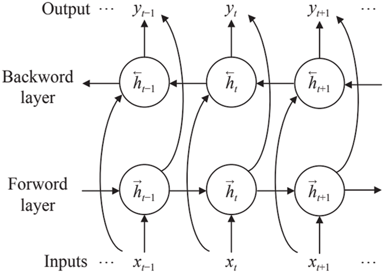
Figure 3: Bidirectional RNN model diagram
In the above formula,
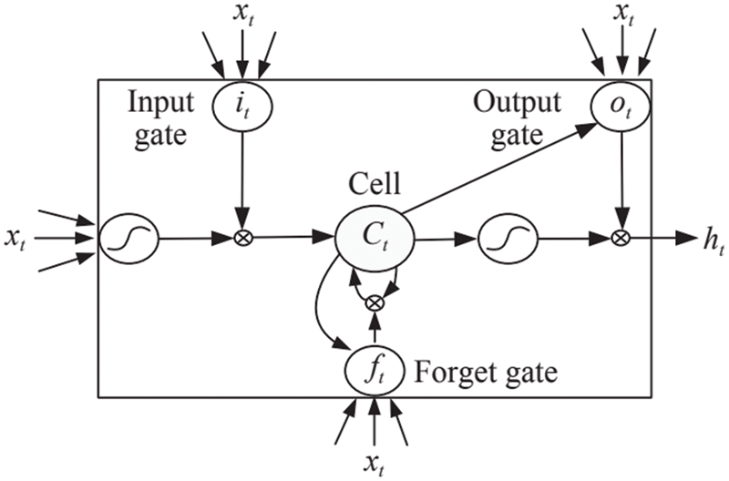
Figure 4: LSTM cell
The input of the Bi-LSTM layer is the feature vector after BIA and GIA. The Bi-LSTM layer adopts a single-layer bidirectional LSTM structure, which contains a hidden layer with 128 nodes. To increase the robustness of model network nodes and reduce the complex co-adaptation relationship between neurons, we add a dropout layer between the Bi-LSTM layer and the FC layer to mask neurons with a certain probability randomly.
We selected four datasets for experiments. We pre-process the dataset and then select accuracy, unweighted f1-score, and unweighted average recall as evaluation criteria. Finally, we conducted experiments on without IBs, 24 and 10 IBs, respectively, and compared them with different algorithms.
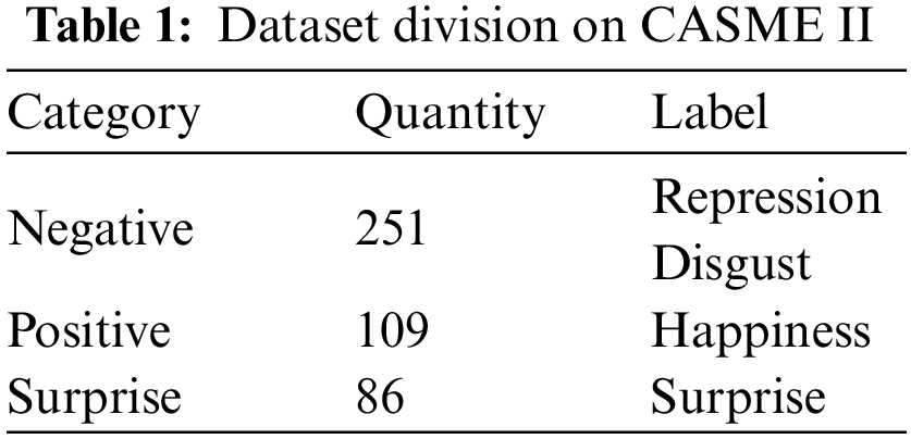
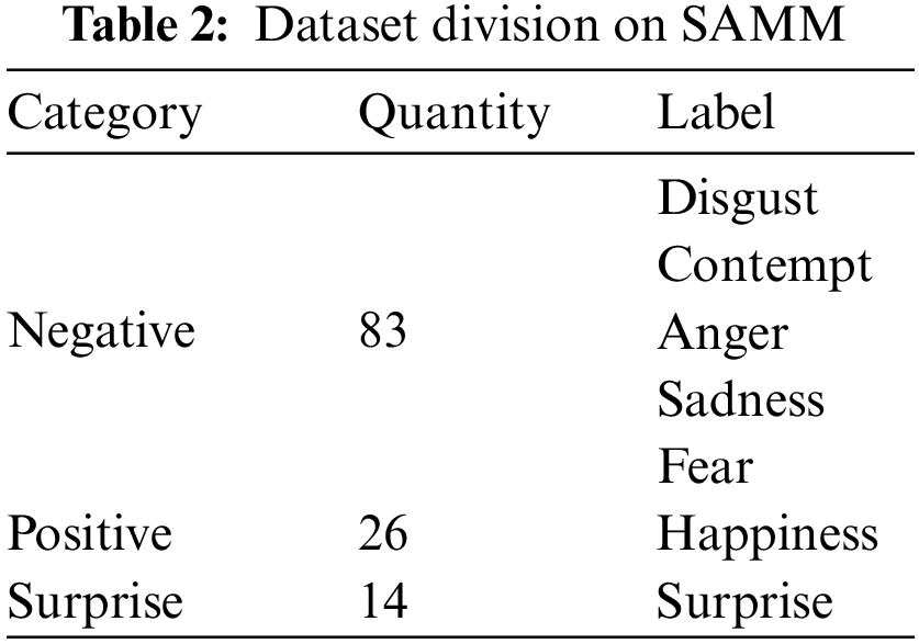
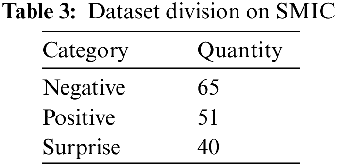
Four datasets, CASME II, SAMM, SMIC and MEGC, were selected for the experiment. In the experiment, we divided expressions into three categories: negative, positive and surprise.
The CASME II [36] dataset was established by the team of Fu Xiaolan, Institute of Psychology, Chinese Academy of Sciences. The CASME II dataset employs a 200 fps high-speed camera with a frame size of 640 × 480 pixels. There are 255 samples in the dataset, the average age of the participants is 22 years old, and the total number of subjects is 24. The dataset includes emotion labels corresponding to each subject sample and video sequence annotations with the onset frame, apex frame and offset frame [37–39]. Labels include depression, disgust, happiness, surprise, fear, sadness, and others. In the experiment, we divided the CASME II dataset into a new division, and the division results are shown in Table 1.
The SAMM [40] dataset has 149 video clips captured by 32 participants from 13 countries. The participants were 17 white British, accounting for 53.1% of the participants; also included 3 Chinese, 2 Arabs, and 2 Malays, in addition to Spanish, Pakistani, Arab, African Caribbean 1 person each, a British African, an African, a Nepalese, and an Indian. The average age of the participants was 33.24 years, with a gender-balanced number of male and female participants. There were significant differences in the race and age of the participants, and the imbalance of the label classes was also evident. The SAMM dataset has a 200 fps high frame rate camera with a resolution of 960 × 650 per frame [41–43]. The dataset is accompanied by the positions of the onset frame, offset frame and apex frame of MEs, as well as emotion labels and action unit information. Labels include disgust, contempt, anger, sadness, fear, happiness, surprise,and others. In the experiment, we divided the SAMM dataset into a new division, and the division results are shown in Table 2.
The SMIC dataset consists of 16 participants and 164 ME clips. Among the volunteers were 8 Asians and 8 Caucasians. The SMIC dataset has a 100 fps camera and a resolution of 640 × 480 per frame [44,45]. The SMIC dataset includes three categories: negative, positive, and surprised, and we do not re-segment in the experiments. The SMIC dataset classification is shown in Table 3.
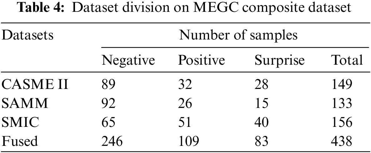
The MEGC composite dataset has 68 volunteers, including 24 from the CASME II dataset, 28 from the SAMM dataset, and 16 from the SMIC dataset. The classification of the composite dataset is shown in Table 4.
Apex frames are annotated in the CASME II and SAMM datasets. Still, in the experiment we found that some datasets are not accurate in the annotation of apex frames and are even mislabeled. In addition, there is no Apex frame information in the SMIC dataset. Therefore it is necessary to re-label apex frames [46]. In the experiments, we obtain the apex frame position by calculating the absolute pixel difference of the gray value between the current frame and the onset and offset frames. To reduce the interference of image noise, we simultaneously calculate the absolute value of the pixel difference between the adjacent frame and the current frame. Then, We divide the two values. Finally, the difference value between each frame and the onset frame and the offset frame is obtained, and the frame with the most considerable difference value is selected as the apex frame.
As in Eqs. (16) and (17),
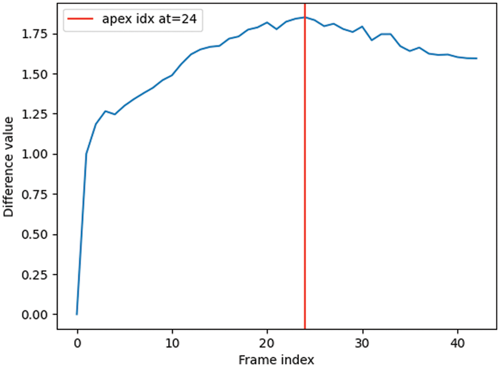
Figure 5: The change process of the difference value of different frames in the ME video. The place with the most immense difference value, that is, the position of the red vertical line, represents the position of the apex frame
After determining the vertex frame, we then use the temporal interpolation model (TIM) [47] to process the video frames from the onset frame to the apex frame into a fixed input sequence of 10 frames. We use Local Weighted Mean Transformation (LWMT) [48] on the 10-frame sequence. The faces are aligned and cropped at the positions of the eyes in the first frame in the same video, and the video frames are normalized to 224 × 224 pixels by bilinear interpolation [49]. In determining 24 facial IBs, we first use face_recognition to get 72 facial keys. After analyzing the face key points, we select 24 facial motion IPs and generate 24 IBs from 24 IPs. In the experiment of determining 10 facial IBs, we first use face_recognition to get 72 facial keys. After analyzing the key points on the face, we select 10 representative IPs and generate 10 IBs from 10 IPs. Finally, we put the pre-processed video frames and the corresponding IBs of each frame into the model for training.
4.3 Experimental Evaluation Criteria
Due to the small sample size of ME datasets, to ensure the accuracy of the experiment, we choose Leave One Subject Out (LOSO) [50]. That is, the dataset is divided according to the subjects, and all videos of one subject are selected each time for testing and the remaining fold training. Until all folds are involved in the test. Finally, all test results are combined and used as the final experimental result.
We adopt the evaluation metrics of
The training uses the Adam optimizer; the learning rate is 0.0001; the number of iterations epoch is set to 100; the training batch_size is set to 16. Because the ME dataset sample size is small, it is prone to overfitting. To improve the robustness and generalization ability of the model, we take the regularized L2 norm for the model parameters and add λ times the L2 parameter norm to the loss function. After many experiments, it is shown that the model works best when λ is set to 0.00001. In addition, we add random rotation and random cropping with degrees from −8 to 8 for data augmentation in our experiments.
4.4.1 Experimental Results on CASME II Dataset
The experimental results are shown in Table 5. In the CASME II dataset, the average accuracy of LOSO without IBs is 0.7364,
The confusion matrix of not using IBs, using 24 IBs and using 10 IBs is shown in Figs. 6a–6c. The confusion matrices of the three methods show commonality in the CASME II dataset. From the confusion matrix, we found that the prediction results of the three methods are more distributed near “negative” and “surprise”, and the accuracy is relatively high. It is mainly caused by the unbalanced distribution of the datasets. Because it is difficult to trigger the “positive” ME in the collection of the CASME II dataset, the number of dataset labels as “negative” and “surprised” is much larger than that of “positive”. It leads to the imbalance of dataset distribution, which affects the training accuracy.
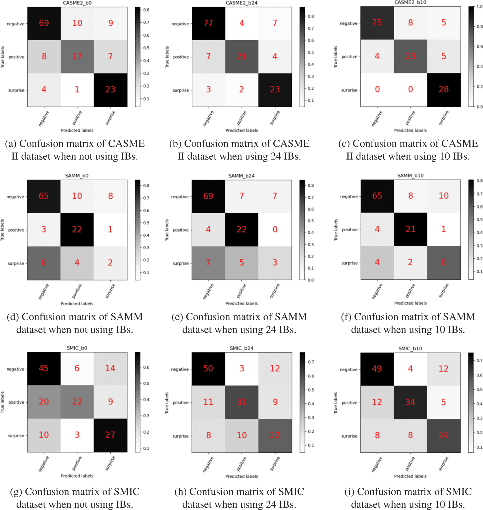
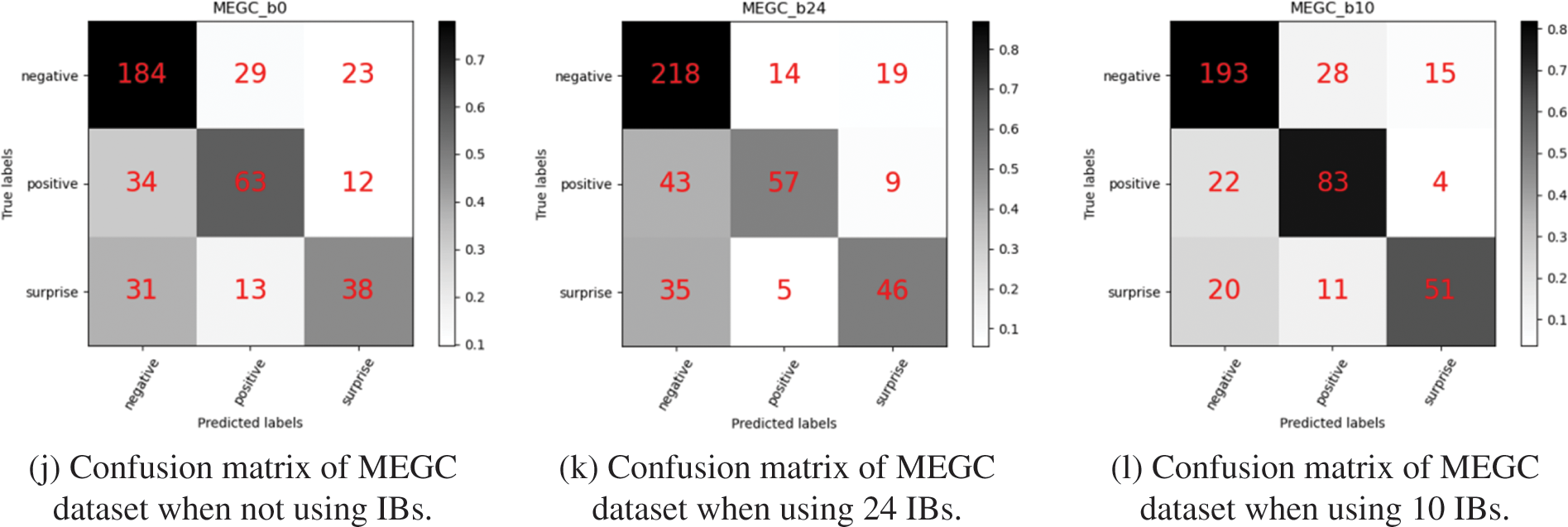
Figure 6: Confusion matrix results on CASME II, SAMM, SMIC and MEGC datasets. We have experimented with 24, 10 IBs, and without IBs on datasets. The experimental results show that using IBs can effectively increase the robustness and recognition effect of the model. Simultaneously, 10 IBs work best
4.4.2 Experimental Results on SAMM Dataset
The experimental results are shown in Table 5. In the SAMM dataset, the average accuracy of LOSO without IBs is 0.7235,
The confusion matrix of not using IBs, using 24 IBs and using 10 IBs is shown in Figs. 6d–6f. In the confusion matrix, we can see that the sample number of “surprise” expressions in the SAMM dataset is tiny, which is one of the reasons why the
4.4.3 Experimental Results on SMIC Dataset
The experimental results are shown in Table 5. In the SMIC dataset, the average accuracy of LOSO without IBs is 0.6025,
The confusion matrix of not using IBs, using 24 IBs and using 10 IBs is shown in Figs. 6g–6i. The accuracy of the SMIC dataset is lower than that of the CASME II and SAMM datasets, mainly due to the lower frame rate and pixels captured by SMIC. In addition, the shooting environment of the SMIC dataset is relatively dark, and the interference of the noise environment is also more than that of the CASME II and SAMM datasets. In the SMIC dataset, by comparing the confusion matrix of the experimental results of adding without IBs, adding 24 IBs and adding 10 IBs, we can find that adding IBs can increase the accuracy of model recognition, especially for the recognition performance of “positive”. It is because the addition of IBs with an attention mechanism increases the ability to extract facial detail features of ME.
4.4.4 Experimental Results on MEGC Composite Dataset
The experimental results are shown in Table 5. In the MEGC composite dataset, the average accuracy of LOSO without IBs is 0.6674,
Confusion matrices without IBs, 24 and 10 IBs are used, as shown in Figs. 6j–6l. The MEGC composite dataset has high requirements on the robustness of the model due to the fusion of three datasets with considerable differences. Compared with without IBs, the confusion matrix with IBs shows higher prediction accuracy in negative expressions. Simultaneously, in the confusion matrix, we also found that the prediction accuracy of negative expressions was the highest when using 24 blocks. It is because negative expressions are mainly eyebrow and eye movements. The 24 IBs have more points at the eyebrows and eyes, so more details are extracted from the face. However, paying too much attention to local details makes the overall robustness of the model worse, which is also why the overall accuracy of 10 IBs is higher than that of 24 IBs.
The comparison of recognition effects of different algorithms is shown in Table 6. The improved algorithm model has the best performance when the number of IBs is 10. The data in Table 6 shows that the accuracy of the model of 10 IBs has been relatively improved compared with the previous recognition algorithms, in which the
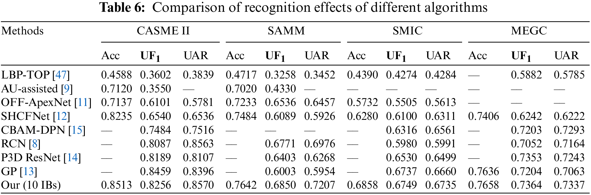
It is because the GP model is an improved algorithm based on an evolutionary algorithm, which has a good effect on extracting the features of ME sequences that change over time. However, this model only extracts global features and does not consider that different parts of the face have different weights in MER. The CBAM-DPN model adds channel and spatial attention to the feature extraction of local details of MEs. But it only relies on the onset and apex frames for identification and ignores the valuable ME information in other consecutive frames. The P3D ResNet can use the optical flow to extract sequence information. This model considers the spatial and temporal information in consecutive frames. However, it does not take into account the variability of different facial parts.
Aiming at the characteristics of short duration and small movement range of ME, we propose a recognition method combining the GIA and BIA framework. In the BIA framework, the ME frames will be cropped into blocks. we perform ablation experiments on uncropped, cropped into 24 and 10 blocks. Considering that the ME dataset is a small sample and prone to over-fitting, we first extract the essential features from the pre-processed ME video frames through VGG16; The global and local features are extracted by GIA and BIA; Then, the sequence information of each frame is extracted by Bi-LSTM; Finally, it is classified by three FC layers. Experiments show that the combination of attention networks with IBs and Bi-LSTM can effectively extract useful spatial information and sequence information from video frames with small action amplitude. It show high accuracy in the experiment. Among them, the model effect is the best when there are 10 IBs. However, the small sample size of ME datasets, generally short duration and low intensity, are still the main reasons for the low experimental recognition rate, which is particularly obvious in the confusion matrix. Although the method in this paper uses TIM to process a fixed input sequence, the low efficiency of the model still needs to be solved due to the use of multiple video frames for feature extraction.
In future research, for the problem of a small sample size of datasets, the quality and quantity of ME datasets need to be further improved. For problems with low intensity of MEs, the next step is to maximize the use of the dataset sequence by doing TIM simultaneously between the video onset frame to apex frame and apex frame to offset frame. In addition, The range of IB can be adjusted according to future experiments. The selection of IBs should be as representative as possible and with high anti-interference.
Acknowledgement: Firstly, I would like to thank Mr. Zhu Wenqiu for his guidance and suggestions on the research direction of my paper. At the same time, I am also very grateful to the reviewers for their useful opinions and suggestions, which have improved the article.
Funding Statement: This work is partially supported by the National Natural Science Foundation of Hunan Province, China (Grant Nos. 2021JJ50058, 2022JJ50051), the Open Platform Innovation Foundation of Hunan Provincial Education Department (Grant No. 20K046), The Scientific Research Fund of Hunan Provincial Education Department, China (Grant Nos. 21A0350, 21C0439, 19A133).
Author Contributions: Conceptualization, Z. W. Q and L. Y. S; methodology, Z. W. Q; validation, Z. W. Q, L. Y. S, Z. Z. G and L. Q; formal analysis, Z. W. Q and Z. Z. G; investigation, L. Y. S; resources, Z. W. Q; data curation, L. Q; writing—original draft preparation, Z. W. Q and L. Y. S; writing—review and editing, Z. W. Q and L. Y. S; visualization, Z. Z. G; supervision, L. Q; project administration, Z. W. Q; funding acquisition, Z. W. Q and Z. Z. G. All authors have read and agreed to the published version of the manuscript.
Availability of Data and Materials: The data used to support the findings of this study are included within the article.
Conflicts of Interest: The authors declare that they have no conflicts of interest to report regarding the present study.
References
1. M. F. Hashmi, B. K. K. Ashish, V. Sharma, A. G. Keskar, N. D. Bokde et al., “LARNet: Real-time detection of facial micro expression using lossless attention residual network,” Sensors, vol. 21, no. 4, pp. 1098, 2021. [Google Scholar] [PubMed]
2. E. A. Haggard and K. S. Isaacs, “Micromomentary facial expressions as indicators of ego mechanisms in psychotherapy,” in Methods of Research in Psychotherapy, 1st ed., vol. 1. Boston, MA, USA: Springer, pp. 154–165, 1966. [Google Scholar]
3. P. Ekman and E. L. Rosenberg, “Basic and applied studies of spontaneous expression using the facial action coding system (FACS),” in What the Face Reveals, 2nd ed., vol. 70. New York, NY, USA: Oxford University Press, pp. 21–38, 2005. [Google Scholar]
4. X. B. Nguyen, C. N. Duong, X. Li, S. Gauch, H. S. Seo et al., “Micron-BERT: BERT-based facial micro-expression recognition,” in Proc. of the IEEE/CVF Conf. on Computer Vision and Pattern Recognition, Vancouver, BC, Canada, pp. 1482–1492, 2023. [Google Scholar]
5. L. Cai, H. Li, W. Dong and H. Fang, “Micro-expression recognition using 3D DenseNet fused squeeze-and-excitation networks,” Applied Soft Computing, vol. 119, no. 1, pp. 108594–108606, 2022. [Google Scholar]
6. T. Pfister, X. Li, G. Zhao and M. Pietikäinen, “Recognising spontaneous facial micro-expressions,” in Proc. of ICCV, Barcelona, BCN, Spain, pp. 1449–1456, 2011. [Google Scholar]
7. G. Zhao and M. Pietikainen, “Dynamic texture recognition using local binary patterns with an application to facial expressions,” IEEE Transactions on Pattern Analysis & Machine Intelligence, vol. 29, no. 6, pp. 915–928, 2007. [Google Scholar]
8. Z. Xia, W. Peng, H. Q. Khor, X. Feng and G. Zhao, “Revealing the invisible with model and data shrinking for composite-database micro-expression recognition,” IEEE Transactions on Image Processing, vol. 29, no. 1, pp. 8590–8605, 2020. [Google Scholar]
9. H. X. Xie, L. Lo, H. H. Shuai and W. H. Cheng, “AU-assisted graph attention convolutional network for micro-expression recognition,” in Proc. of the 28th ACM MM, Seattle, SEA, USA, pp. 2871–2880, 2020. [Google Scholar]
10. X. R. Li, L. Y. Zhang and S. J. Yao, “Micro-expression recognition method combining feature fusion and attention mechanism,” Computer Science, vol. 49, no. 2, pp. 4–11, 2022. [Google Scholar]
11. Y. S. Gan, S. T. Liong, W. C. Yau, Y. C. Huang and L. K. Tan, “OFF-ApexNet on micro-expression recognition system,” Signal Processing: Image Communication, vol. 74, no. 1, pp. 129–139, 2019. [Google Scholar]
12. J. Huang, X. R. Zhao and L. M. Zheng, “SHCFNet on micro-expression recognition system,” in 13th Int. Cong. on Image and Signal Processing, BioMedical Engineering and Informatics (CISP-BMEI), Chengdu, China, pp. 163–168, 2020. [Google Scholar]
13. W. P. Zhan, M. Jiang, J. F. Yao, K. H. Liu and Q. Q. Wu, “The design of evolutionary feature selection operator for the micro-expression recognition,” Memetic Computing, vol. 14, no. 1, pp. 61–67, 2022. [Google Scholar]
14. H. Tang, L. J. Zhu, S. Fan and H. M. Liu, “Micro-expression recognition based on optical flow method and pseudo three-dimensional residual network,” Signal Processing, vol. 38, no. 5, pp. 1075–1087, 2022. [Google Scholar]
15. R. H. Niu, J. Yang, L. X. Xing and R. B. Wu, “Micro expression recognition algorithm based on convolutional attention module and dual channel network,” Computer Applications, vol. 41, no. 9, pp. 2552–2559, 2021. [Google Scholar]
16. Y. Li, X. Huang and G. Zhao, “Micro-expression action unit detection with spatial and channel attention,” Neurocomputing, vol. 436, no. 1, pp. 221–231, 2021. [Google Scholar]
17. K. M. Goh, C. H. Ng, L. L. Lim and U. U. Sheikh, “Micro-expression recognition: An updated review of current trends, challenges and solutions,” The Visual Computer, vol. 36, no. 3, pp. 445–468, 2020. [Google Scholar]
18. C. Wang, M. Peng, T. Bi and T. Chen, “Micro-attention for micro-expression recognition,” Neurocomputing, vol. 410, no. 8, pp. 354–362, 2020. [Google Scholar]
19. J. Zhu, Y. Zong, H. Chang, L. Zhao and C. Tang, “Joint patch weighting and moment matching for unsupervised domain adaptation in micro-expression recognition,” IEICE Transactions on Information and Systems, vol. 105, no. 2, pp. 441–445, 2022. [Google Scholar]
20. K. Wang, X. Peng, J. Yang, D. Meng and Y. Qiao, “Region attention networks for pose and occlusion robust facial expression recognition,” IEEE Transactions on Image Processing, vol. 29, no. 1, pp. 4057–4069, 2020. [Google Scholar]
21. W. Merghani, A. K. Davison and M. H. Yap, “The implication of spatial temporal changes on facial micro-expression analysis,” Multimedia Tools and Applications, vol. 78, no. 15, pp. 21613–21628, 2019. [Google Scholar]
22. Y. Li, “Face detection algorithm based on double-channel CNN with occlusion perceptron,” Computational Intelligence and Neuroscience, vol. 2022, no. 1, pp. 1687–5265, 2022. [Google Scholar]
23. X. Wang, Z. Guo, H. Duan and W. Chen, “An efficient channel attention CNN for facial expression recognition,” in Proc. of the 11th Int. Conf. on Computer Engineering and Networks, Singapore, pp. 75–82, 2022. [Google Scholar]
24. S. Dong, X. Zhang and Y. Li, “Microblog sentiment analysis method based on spectral clustering,” Journal of Information Processing Systems, vol. 14, no. 3, pp. 727–739, 2018. [Google Scholar]
25. Z. Yang, H. Wu, Q. Liu, X. Liu, Y. Zhang et al., “A self-attention integrated spatiotemporal LSTM approach to edge-radar echo extrapolation in the internet of radars,” ISA Transactions, vol. 132 pp. 155–166, 2023. https://doi.org/10.1016/j.isatra.2022.06.046 [Google Scholar] [PubMed] [CrossRef]
26. A. Singh, S. K. Dargar, A. Gupta, A. Kumar, A. K. Srivastava et al., “Evolving long short-term memory network-based text classification,” Computational Intelligence and Neuroscience, vol. 2022, no. 1, pp. 1–11, 2022. [Google Scholar]
27. Z. Yang, Q. Liu, H. Wu, X. Liu and Y. Zhang, “CEMA-LSTM: Enhancing contextual feature correlation for radar extrapolation using fine-grained echo datasets,” Computer Modeling in Engineering & Sciences, vol. 135 pp. 45–64, 2023. https://doi.org/10.32604/cmes.2022.022045 [Google Scholar] [CrossRef]
28. S. Hochreiter, “LSTM can solve hard long term lag problems,” in Neural Information Processing Systems (Nips 9), 1997. [Google Scholar]
29. L. Singh, “Deep bi-directional LSTM network with CNN features for human emotion recognition in audio-video signals,” International Journal of Swarm Intelligence, vol. 7, no. 1, pp. 110–122, 2022. [Google Scholar]
30. S. C. Ayyalasomayajula, “A novel deep learning approach for emotion classification,” M.S. Dissertation, University of Ottawa, Canada, 2022. [Google Scholar]
31. R. Kavitha, P. Subha, R. Srinivasan and M. Kavitha, “Implementing OpenCV and Dlib open-source library for detection of driver’s fatigue,” In: Innovative Data Communication Technologies and Application, 1st ed., vol. 1, pp. 353–367, Singapore: Springer, 2022. [Google Scholar]
32. S. Reddy Boyapally, “Facial recognition and attendance system using Dlib and Face_Recognition libraries, pp. 1–6, 2021. [Online]. Available: https://ssrn.com/abstract=3804334 [Google Scholar]
33. X. Yang, C. Liu, L. L. Xu, Y. K. Wang, Y. P. Dong et al., “Towards effective adversarial textured 3D meshes on physical face recognition,” in Proc. of the IEEE/CVF Conf. on Computer Vision and Pattern Recognition, pp. 4119–4128, 2023. [Google Scholar]
34. J. Luo and X. Zhang, “Convolutional neural network based on attention mechanism and Bi-LSTM for bearing remaining life prediction,” Applied Intelligence, vol. 52, no. 1, pp. 1076–1091, 2022. [Google Scholar]
35. W. J. Yan, X. Li, S. J. Wang, G. Zhao, Y. J. Liu et al., “CASME II: An improved spontaneous micro-expression database and the baseline evaluation,” PLoS One, vol. 9, no. 1, pp. 86041, 2014. [Google Scholar]
36. H. Li, M. Sui, Z. Zhu and F. Zhao, “MMNet: Muscle motion-guided network for micro-expression recognition,” in Computer Vision and Pattern Recognition, pp. 1–8, 2022. https://doi.org/10.48550/arXiv.2201.05297 [Google Scholar] [CrossRef]
37. W. Jin, X. Meng, D. Wei, W. Lei and W. Xinran, “Micro-expression recognition algorithm based on the combination of spatial and temporal domains,” High Technology Letters, vol. 27, no. 3, pp. 303–309, 2021. [Google Scholar]
38. P. Rathi, R. Sharma, P. Singal, P. S. Lamba and G. Chaudhary, “Micro-expression recognition using 3D-CNN layering,” in AI-Powered IoT for COVID-19, 1st ed., vol. 1. Florida, FL, USA: CRC Press, pp. 123–140, 2020. [Google Scholar]
39. A. K. Davison, C. Lansley, N. Costen, K. Tan and M. H. Yap, “SAMM: A spontaneous micro-facial movement dataset,” IEEE Transactions on Affective Computing, vol. 9, no. 1, pp. 116–129, 2016. [Google Scholar]
40. A. J. R. Kumar and B. Bhanu, “Micro-expression classification based on landmark relations with graph attention convolutional network,” in Proc. of the IEEE/CVF Conf. on Computer Vision and Pattern Recognition (CVPR), New York, NY, USA, pp. 1511–1520, 2021. [Google Scholar]
41. L. Lei, T. Chen, S. Li and J. Li, “Micro-expression recognition based on facial graph representation learning and facial action unit fusion,” in Proc. of the IEEE/CVF Conf. on Computer Vision and Pattern Recognition (CVPR), New York, NY, USA, pp. 1571–1580, 2021. [Google Scholar]
42. K. H. Liu, Q. S. Jin, H. C. Xu, Y. S. Gan and S. T. Liong, “Micro-expression recognition using advanced genetic algorithm,” Signal Processing: Image Communication, vol. 93, pp. 116153, 2021. [Google Scholar]
43. X. Zhang, T. Xu, W. Sun and A. Song, “Multiple source domain adaptation in micro-expression recognition,” Journal of Ambient Intelligence and Humanized Computing, vol. 12, no. 8, pp. 8371–8386, 2021. [Google Scholar]
44. G. Chinnappa and M. K. Rajagopal, “Residual attention network for deep face recognition using micro-expression image analysis,” Journal of Ambient Intelligence and Humanized Computing, vol. 13, no. 1, pp. 117, 2022. [Google Scholar]
45. X. Jiang, Y. Zong, W. Zheng, J. Liu and M. Wei, “Seeking salient facial regions for cross-database Micro-expression recognition,” in the 2022 26th Int. Conf. on Pattern Recognition (ICPR), Montreal, QC, Canada, pp. 1–7, 2021. [Google Scholar]
46. S. Zhao, H. Tao, Y. Zhang, T. Xu, K. Zhang et al., “A two-stage 3D CNN based learning method for spontaneous micro-expression recognition,” Neurocomputing, vol. 448, no. 1, pp. 276–289, 2021. [Google Scholar]
47. K. H. Liu, Q. S. Jin, H. C. Xu, Y. S. Gan and S. T. Liong, “Micro-expression recognition using advanced genetic algorithm,” Signal Processing: Image Communication, vol. 93, no. 1, pp. 116153, 2021. [Google Scholar]
48. S. Cen, Y. Yu, G. Yan, M. Yu and Y. Kong, “Micro-expression recognition based on facial action learning with muscle movement constraints,” Journal of Intelligent & Fuzzy Systems, vol. 2021, no. 1, pp. 1–17, 2021. [Google Scholar]
49. Z. Xie, L. Shi, S. Cheng, J. Fan and H. Zhan, “Micro-expression recognition based on deep capsule adversarial domain adaptation network,” Journal of Electronic Imaging, vol. 31, no. 1, pp. 013021, 2022. [Google Scholar]
50. D. Chicco and G. Jurman, “The advantages of the matthews correlation coefficient (MCC) over F1 score and accuracy in binary classification evaluation,” BMC Genomics, vol. 21, no. 1, pp. 1–13, 2020. [Google Scholar]
51. A. Rosenberg, “Classifying skewed data: Importance weighting to optimize average recall,” in ISCA’s 13th Annual Conf., Portland, PO, USA, pp. 2242–2245, 2012. [Google Scholar]
Cite This Article
 Copyright © 2023 The Author(s). Published by Tech Science Press.
This work is licensed under a Creative Commons Attribution 4.0 International License , which permits unrestricted use, distribution, and reproduction in any medium, provided the original work is properly cited.
 Downloads
 Citation Tools