Visualization for Explanation of Deep Learning-Based Fault Diagnosis Model Using Class Activation Map

1  Introduction

Due to its wide range of constant power speed, better dynamic performance, easy maintenance, and other advantages [1], permanent magnet synchronous motor has been widely used in social production because of its extensive speed range, excellent dynamic performance, and relatively simple structure [2]. Therefore, it is of great social and economic significance to analyze and diagnose the faults of PMSM.

To date, the diagnosis methods of motor faults are mainly based on three aspects: model, signal, and data-driven method [3]. The model-based method usually requires establishing a mathematical model and using equations to describe the troubled motor’s rigid structure accurately. Modeling methods include methods based on classical state estimation or process parameter estimation [4], finite element method, etc. [5,6]. This method conducts fault analysis based on the model, which has the advantage of going deep into the essence of motor operation but has the disadvantage of relying on an accurate mathematical model of the motor. The second approach is signal-based and does not rely on precise mathematical models. At present, there are several methods to diagnose different types of motor faults by signal: (1) Spectrum analysis; (2) Vector decomposition method [7]; (3) Time-frequency analysis method [8], etc. But these methods require corresponding expertise. The method of motor fault diagnosis based on data drive originates from the extensive application and progress of massive AI technologies in different fields [9], such as aerospace [10], industrial production [11] and construction engineering [12], and so on. Unlike the signal-based fault diagnosis method, a neural network does not need the corresponding expert knowledge. It only needs to import a large amount of data to train the neural network. After its related parameters are fixed, the fault diagnosis of different types of motor faults can be carried out.

Various deep and machine-learning algorithms have been widely used in mechanical fault diagnoses [13]. Literature [14] and literature [15] proposed dislocated time series convolutional neural network (DTS-CNN) and hierarchical convolutional neural networks (TICNN) to detect motor bearing faults by processing motor vibration signals. In literature [16], the stator current of PMSM is transformed by fast fourier transform (FFT), and its amplitude is imported into one-dimensional CNN for training to diagnose the demagnetization fault and bearing fault of PMSM. Tamilselvan and Wang proposed a fault diagnosis method of DNN based on a constrained Boltzmann machine is offered. Still, this method requires many sensors to collect related signals. Each layer is treated as a deep network structure in this method and trained. Although this method has an excellent diagnostic effect on machine faults, it has a lot of background noise which is difficult to eliminate.

Literature [17] proposed an uncrewed aerial vehicle (UAV) image target detection based on the improved you only look once (YOLO) algorithm. From the perspective of model efficiency, it effectively solved the real-time target detection problem of multi-scale targets by using target box dimension clustering, pre-training network classification, multi-scale detection training, and changing the screening rules of candidate boxes. Literature [18] proposed an automatic weed detection system based on UAV images based on CNN. The overall accuracy of the convolutional neural network-learning vector quantization (CNN-LVQ) model developed for weed detection was significantly improved through strict hyperparameter adjustment. Literature [19] optimized the climate depth long short-term memory (CDLSTM) model for predicting temperature and rainfall in Himalayan states. It uses Facebook’s FB-Prophet model to predict and evaluate the performance of the developed CDLSTM model. It has higher accuracy and a lower error rate than the previous algorithm. Literature [20] proposed a brain tumor classification model (DCNNBT) based on a new deep convolutional neural network. By scaling the image resolution, depth of layers, and width of channels and strictly optimizing the hyperparameters, the model achieved a classification accuracy of up to 99.18%, which was significantly higher than other studies based on the same database. Literature [21] proposed the application of a five-layer CNN to large-scale plant classification in the natural environment. Plant identification based on experimental data has high accuracy. The model achieved the highest recognition rate of 96% on the NU108 dataset, and the accuracy of NU101 drone images reached 97.8%. However, most fault diagnosis methods based on deep learning are black boxes. It is impossible to know which image features have been classified based on the neural network, and the mapping established by the neural network needs descriptive analysis. Therefore, a complete CNN and Grad-CAM method for motor fault diagnosis is proposed in this paper, and demagnetizing faults and eccentricity faults of PMSMs are diagnosed.

The major innovations of the article are as follows:

1. Multi-scale feature fusion module, attention mechanism, and atrous convolution pyramid are added to the traditional ResNet network, which enhances the feature extraction capability of the model and improves the fault diagnosis accuracy of the motor. In this paper, a multi-scale feature fusion module, attention mechanism, and atrous convolution pyramid are added to the traditional ResNet network, which enhances the feature extraction capability of the model and improves the fault diagnosis accuracy of the motor.

2. Grad-CAM is introduced to solve the “black box” problem in the fault diagnosis process of the CNN, and the diagnosis based on the features of the image is studied, and the original frequency signal corresponding to the features on the image is determined.

The rest of this paper is arranged as follows: The second section introduces the establishment of symmetrical and asymmetric PMSM models on the finite element software AltairFlux, and co-simulation with MATLAB to obtain the current, torque and speed data of different faulty motors during operation. The third section converts the time-domain signals of stator currents of other defective motors into frequency-domain signals and converts the frequency-domain signals into grayscale images to make data sets and convolutional neural network architecture based on attention channel, multi-scale feature fusion module, and ASPP was constructed, and training parameters were configured. In the fourth section, the produced data set is imported into the built CNN for training and compared with other algorithms. Then, Grad-cam was used to analyze the gray image of the demagnetization fault and eccentricity fault and find out the fault characteristics of the demagnetization fault and eccentricity fault.

2  Build Different Types of Fault Models of PMSM

AFinite element modeling software-Altair Flux is often used for modeling and simulation in the electromagnetic field [22]. Taking it to create a model can be divided into four steps: establishing the motor geometric model, setting the physical properties, setting the model-solving parameters and solving them, and processing the results. At every step of the process, Flux will save relevant files. As long as the “post-processing” is performed to visualize or save the results, the solution results of each parameter can be obtained.

Motor faults can be divided into electrical defects, mechanical faults, magnetic faults, and so on. In this article, the static eccentric responsibility (Se10, Se20) and the demagnetization fault (De25, De50) are taken as examples, and the CNN is built, and the feature visualization technology is used to diagnose these two kinds of faults.

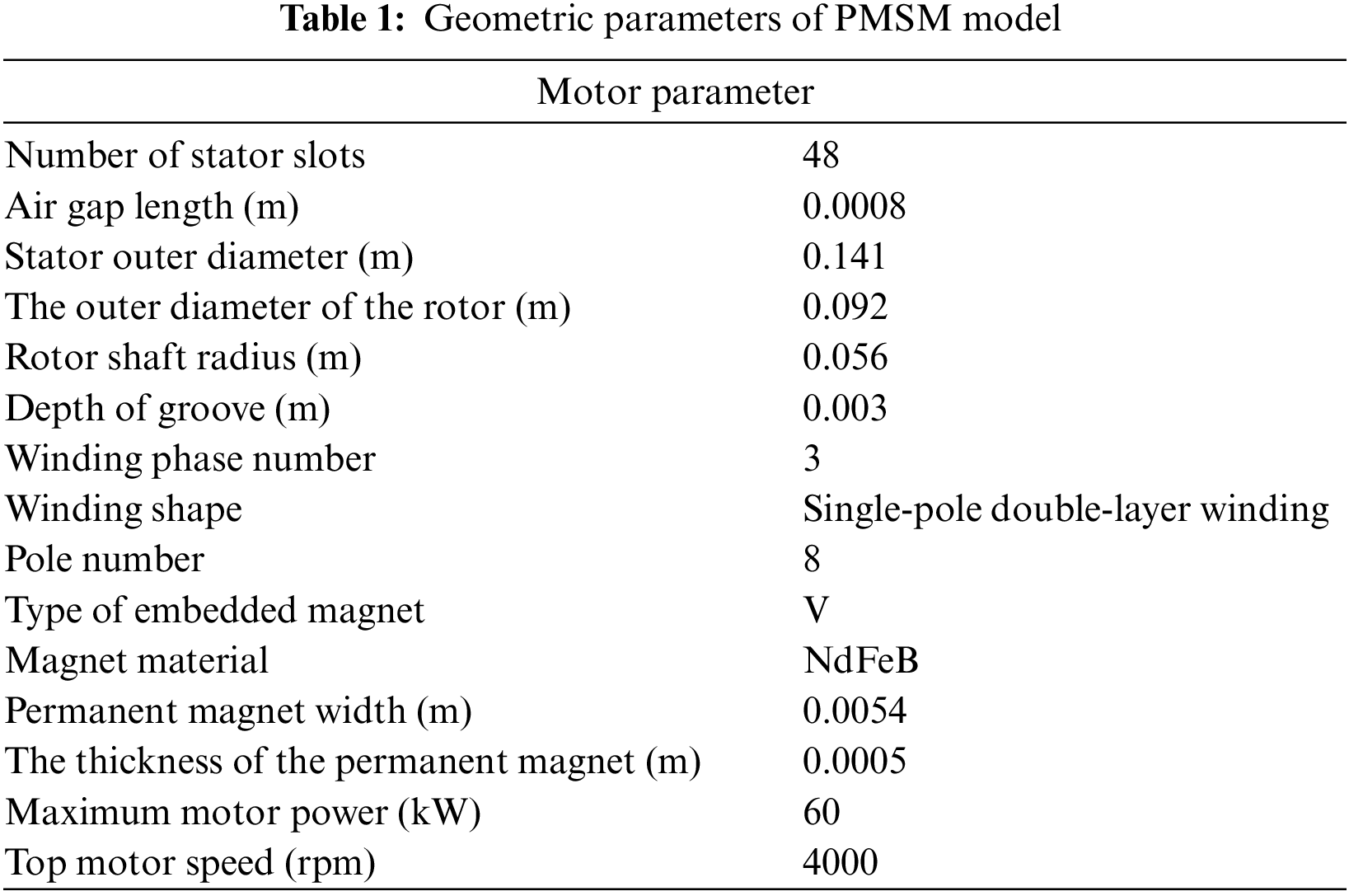
Based on the geometric parameters of PMSM in the Flux official tutorial, this paper redesigned the electrical parts of the motor and the structure of the permanent magnet and established an 8-pole, 48-slot PMSM model, whose structural parameters are shown in Table 1.

2.1 Establishment of PMSM Model for Demagnetization Fault and Eccentricity Fault

When the motor appears to have an eccentric weakness, its topology will become asymmetric. When the strange fault model of the engine is built in Flux, the intact geometric construction of the PMSM needs to be contrived. In this paper, 10% and 20% static eccentricity fault models of permanent magnet synchronous motors are built in Flux. As shown in Fig. 2a, the coordinates Or and Os of the stator center of PMSM and the rotor axis are set as (0.06,0) and (0,0), respectively, so that the distance between them is 0.06 mm (uniform air gap length is 0.6 mm). In this way, the motor model with a 10% static eccentricity fault is obtained Fig. 1b shows the setting method of the PMSM model for 20% eccentric fault. That is, the fixed and rotor axes are set as (0.12,0) and (0.0), respectively, so that the distance between the fixed and rotor axes is 0.12 mm. Then in mechanical properties, set the center of rotation of the rotor to (0.0) so that the center of rotation of the rotor coincides with the axis of the rotor. Thus, the PMSM model with 10% and 20% static eccentricity faults is obtained.

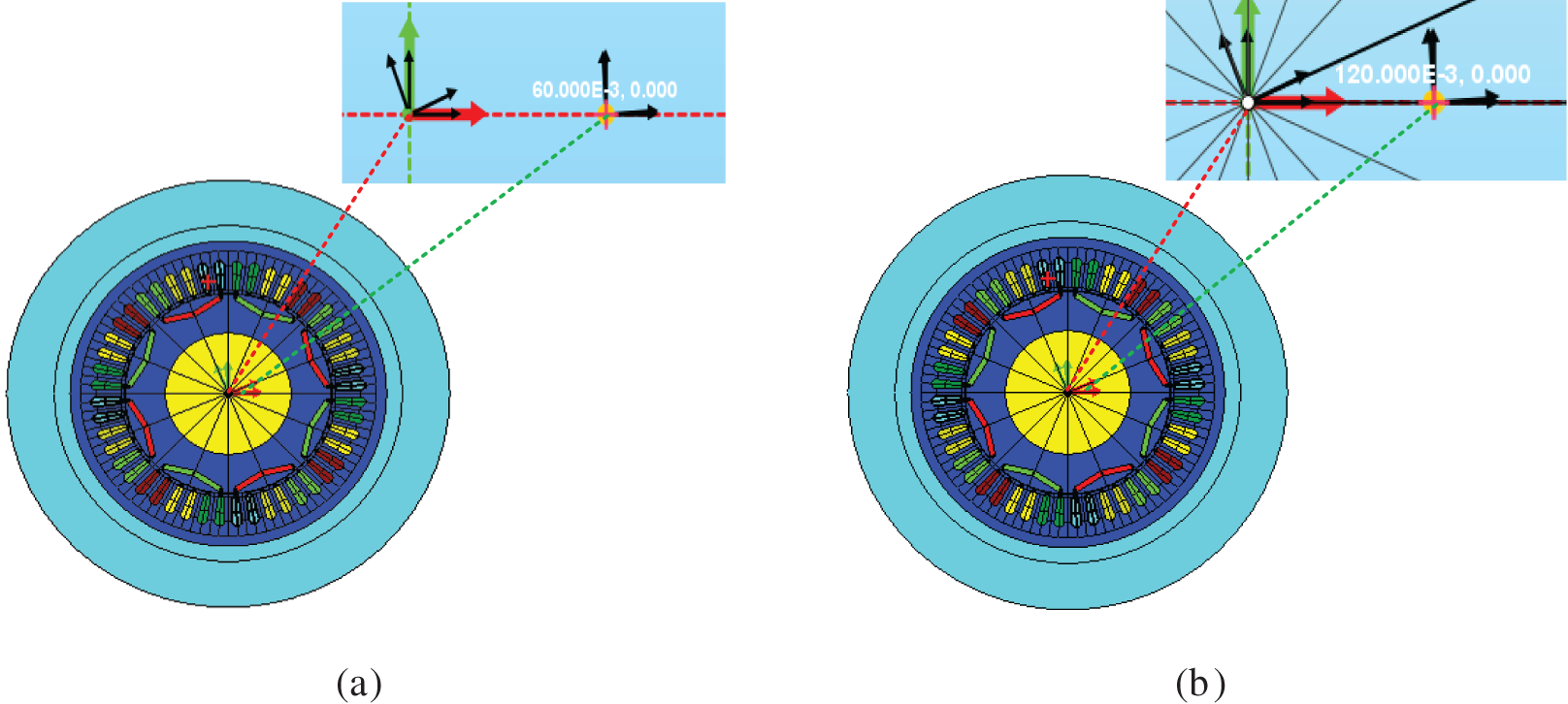
Figure 1: Static eccentric fault motor model: (a) 10% static eccentric; (b) 20% static eccentricity

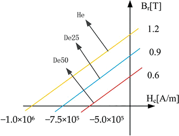
Figure 2: Magnetic curves of NdFeB and its demagnetized materials (operating temperature: 20°C)

Due to its high energy density and low price, neodymium boron (NdFeB) is commonly used to make permanent magnets for permanent magnet synchronous motors. However, it also has the disadvantages that the magnetization intensity is greatly affected by working conditions, and the demagnetization is irreversible. The demagnetization failure of PMSM is usually uniform demagnetization of permanent magnets.

In Flux, it can be described by “Remanent flux density” and “Relative permeability” to the type of permanent magnet and the residual magnetic of permanent magnet materials Br, the slope of the magnetic curve is defined. In this paper, three magnetic curves are defined respectively, which are the magnetic curves of ordinary (He), 25% (De25), and 50% (De50) demagnetized materials. An PMSM model with demagnetization faults of different degrees in permanent magnets on opposite pairs is established.

As shown in Fig. 2, yellow, blue, and red lines in three different colors represent normal, 25% demagnetization, and 50% demagnetization magnetic profile curves of permanent magnets. Their remanence Br can be set to 1.2, 0.9, and 0.6 T, respectively, and their permeability can be set to 1.05. Figs. 3a and 3b respectively represent the sub-densities of permanent magnets with 25% and 50% demagnetization. It can be seen from the figure that the more profound the demagnetization degree of permanent magnets, the more sparse the magnetic densities.

Figure 3: Magnetic density distribution diagram of the permanent magnet of the motor with demagnetizing failure: (a) Demagnetizing 25%; (b) Demagnetizing 50%

2.2 Co-Simulation and Result Analysis

In this paper, finite element models of different types of PMSM established in Altair Flux were imported into a vector control system in MATLAB for co-simulation. Current strategies used in the vector control system id=0 and using the space vector pulse width modulation (SVPWM) motor power supply voltage vector modulation algorithm. Fig. 4 shows the PMSM finite element model in a loop simulation system co-simulated by AltairFlux and MATLAB-Simulink [23].

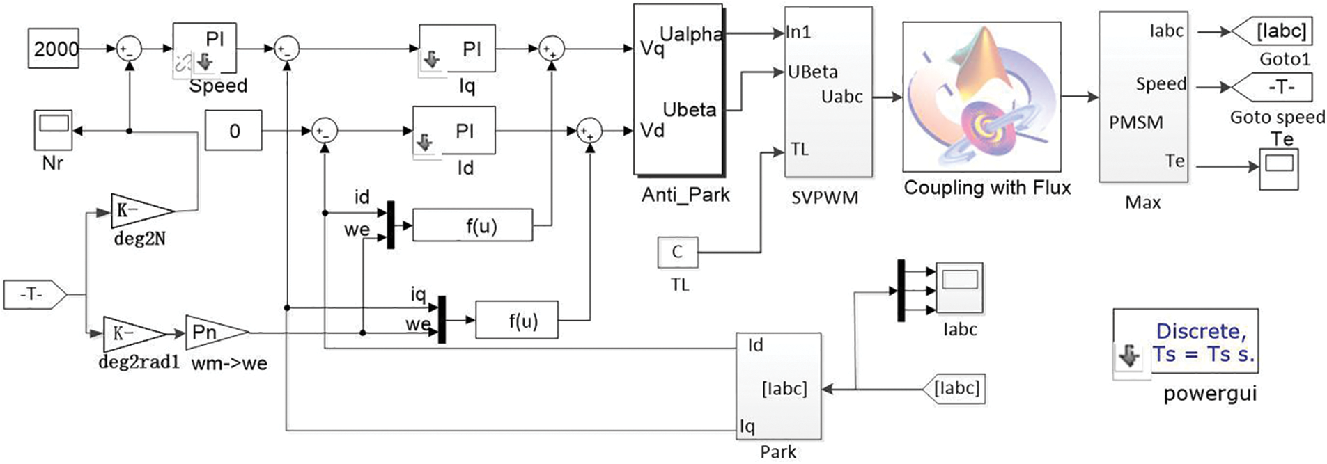
Figure 4: Magnetic curves of NdFeB and its demagnetized materials (operating temperature: 20°C)

Fig. 5 respectively shows the stator three-phase current simulation results of 25% demagnetization, 50% demagnetization, and normal PMSM at a rated speed of 4000 rpm and load 0 N. Figs. 5a–5c are the simulation results of stator currents of three types of motors, respectively. It can be seen from the figure that demagnetization of the engine will increase the time for the motor to enter the steady state. Fig. 5d shows the speed variation of the three motors. It can be seen that demagnetizing failure will increase the time required for the motor speed to reach a steady state. Fig. 5e shows the electromagnetic torque comparison. In the same way, the greater the demagnetizing intensity, the longer the adjustment time required for the motor to reach a steady state and the smaller the electromagnetic torque. In summary, demagnetizing failure is equivalent to increasing the engine load, thus increasing the adjustment time for the motor to reach a steady state.

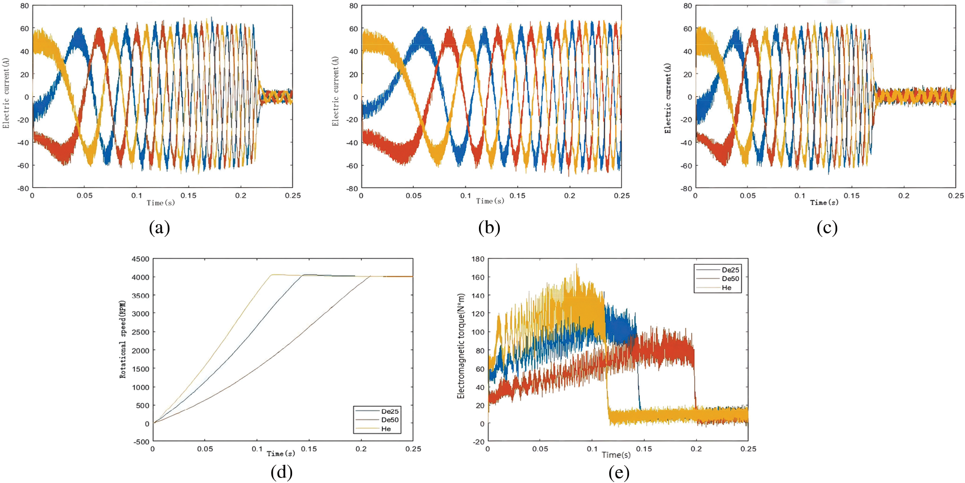
Figure 5: PMSM Simulation results: (a) De25 PMSM stator current; (b) De50 PMSM stator current; (c) Normal PMSM stator current; (d) Speed of comparison; (e) Comparison of electromagnetic torque

Fig. 6 shows the simulation results of typical, 10% eccentric, and 20% strange permanent magnet synchronous motor when the given speed is 4000 rpm, and the load is 0 N.m. Figs. 6a–6c are the simulation results of stator currents of three types of motors, respectively, and (d) and (e) are the comparison of three motor speeds and electromagnetic torques. It can be seen that pure static eccentricity fault has no apparent influence on the stator current, rotational speed, and electromagnetic torque of PMSM [24].

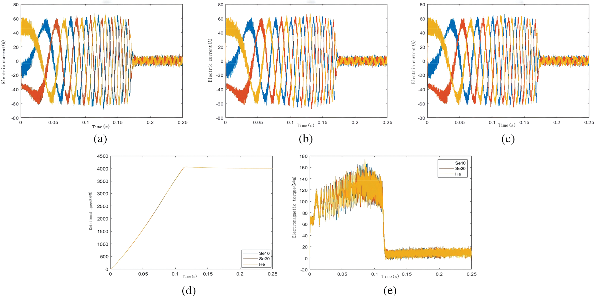
Figure 6: PMSM simulation results: (a) Normal PMSM stator current; (b) Se10 PMSM stator current; (c) Se20 PMSM stator current; (d) Speed of comparison; (e) Comparison of electromagnetic torque

3  Data Set Making and CNN Model Building

3.1 Stator Current FFT Transformation

FFT is a standard signal processing method that can quickly realize signal transformation from a time domain to a frequency domain. Discrete fourier transform (DFT) is the most basic method, digital signal processing of the input signal by frequency fs interval sampling after n times, such as DFT processing of n discrete points get n the plural. Each complex number represents the amplitude and phase information of the frequency component with fs/n as the interval, to obtain the spectrum information of the input signal [25].

For a time-domain discrete signal X(n) with length n, the DFT transformation result is X(k), then:

X(k)=DFT{x(n)}=∑n=0N−1x(n)∗e−j2πNnk,k=0,1,…,N−1(1)

If the following definition is made:

WN=e−j2πN(2)

WNnk=e−j2πNnk(3)

Then X(k) can be expressed as:

X(k)=DFT{x(n)}=∑n=0N−1x(n)∗WNnk,k=0,1,…,N−1(4)

FFT mainly uses periodicity, Symmetry, and scaling of rotation factor to carry out butterfly iterative calculation of DFT to reduce the computation amount of DFT, but its basic properties are still similar to DFT.

In the PMSM fault model built by AltairFlux and MATLAB, the simulation model collected 8000 data points in the time domain signal of stator current at 0.25 s, and the sampling frequency was 32 kHz. The spectrum diagram of the stator three-phase currents of the standard motor, the 25% and 50% demagnetization fault motor, and the 10% and 20% static eccentricity fault motor obtained through the co-simulation is shown in Fig. 7. Since bilateral spectra are symmetrical, only unilateral spectra can be analyzed.

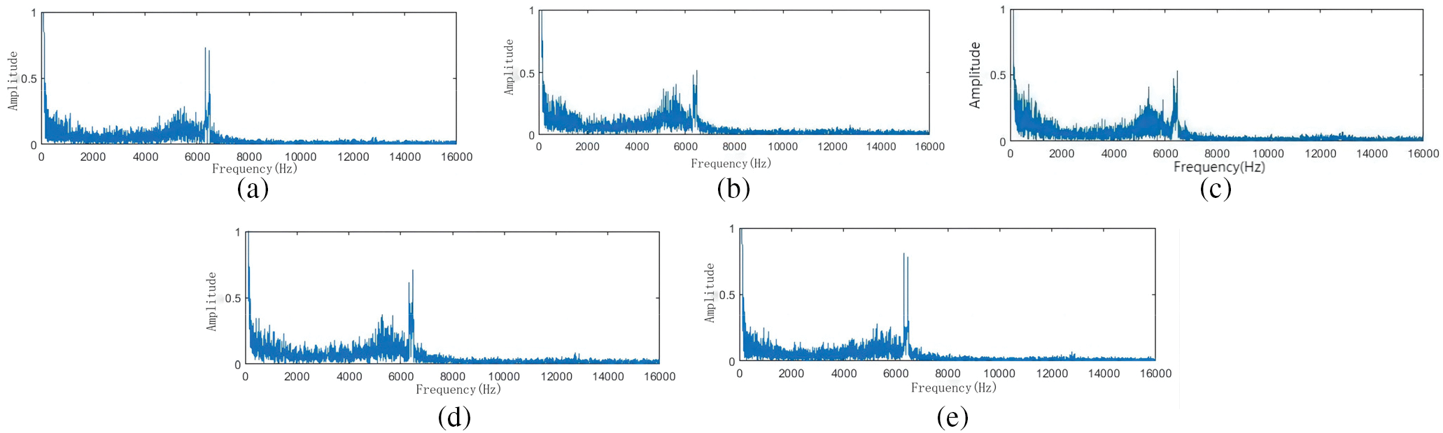
Figure 7: Spectrum diagram of stator current of PMSM with different faults: (a) Normal PMSM; (b) De25 PMSM; (c) De50 PMSM; (d) Se10 PMSM; (e) Se20 PMSM

3.2 The Frequency Domain Signal is Converted into a Gray Image

Because high-dimensional features often contain more data features, this paper first upgraded the frequency domain signal of motor stator current into the two-dimensional gray image, then produced a data set and imported it into CNN [26]. The scattering of data sample values within the range of gray values can be deemed as a probability problem. Because of the significant number theorem, on the condition the amount of data is large enough, the data will obey the Gaussian distribution. Therefore, the mapping function of data scattering into the gray range is set as a one-dimensional Gaussian distribution function in this paper, as shown in the formula (5). Fig. 8 shows the process of image conversion based on the autocorrelation matrix [27].

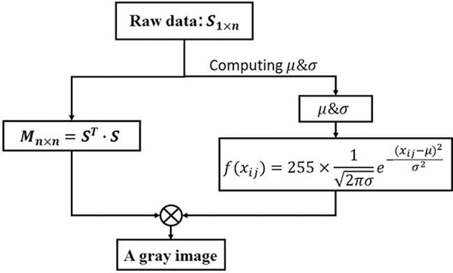
Figure 8: Image conversion flow chart based on autocorrelation matrix

f(xij)=255×12πσe(xij−u)2σ2(5)

where xij are elements in the ith row and the Jth column of the autocorrelation matrix; μ is the mean value of the original data; σ2 is the variance of the original data.

If P(i,j) it represents the intensity of pixels in the generated row I and column j and S(i,1) represents the I-th data point in the original frequency domain signal, then:

P(i,j)=ST(1,j)∗S(i,1)+f(xij)(6)

Therefore, the pixels in the I-th row and J-th column of the grayscale image generated by the image conversion method based on the autocorrelation matrix reflect the intensity of the I-th data point in the original data, and the generated grayscale map is symmetrical about its diagonal.

3.3 Make a Data Set

In this paper, an image conversion method based on an autocorrelation matrix is used to convert the frequency domain signal of motor stator current into a gray-level image. In the spectrum diagram, 500 data points are sampled every 30 data points and dimensionally upgraded. The way of data interception is shown in Fig. 9:

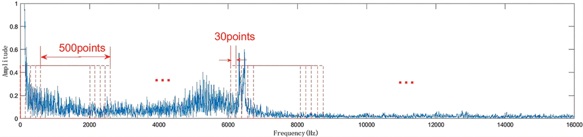
Figure 9: Data interception mode

There are 8000 data points in the time domain signal of single-phase current of different fault motors obtained by co-simulation, and 8000 data points in the bilateral spectrum obtained by FFT. By converting the two-sided range of the three-phase current into the gray image, the original gray image of each type of fault is 793. After data enhancement, 20% of the grayscale images are randomly selected as the test set, and the data set information is shown in Table 2 and the grayscale images converted from frequency domain signals of PMSM with different fault types are shown in Fig. 10.

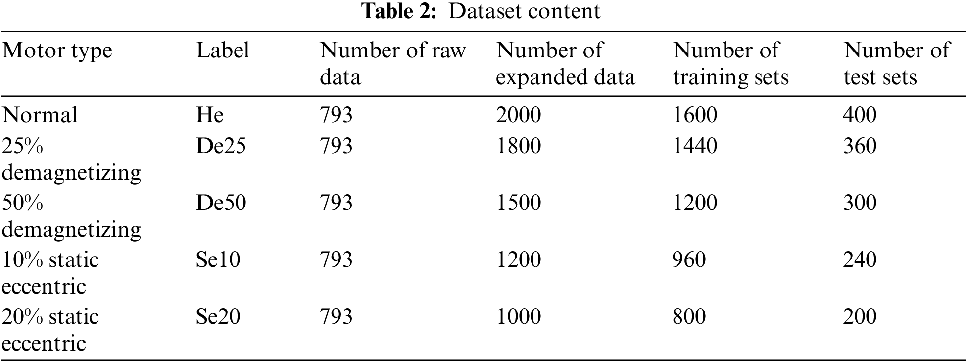
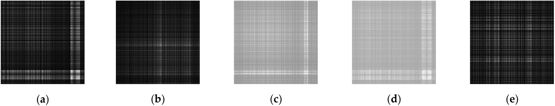
Figure 10: Grayscale image converted from PMSM frequency domain signals of different faults (load is 0 N.m): (a) De25; (b) De50; (c) Normal; (d) Se10; (e) Se20

The training of CNN generally requires large data sets, and reading grayscale images in data sets one by one will occupy a lot of computing resources. In the TensorFlow framework, sample images can be made into TFRecord files to compress the data set into binary coding. During training, it can be decoded and then imported into CNN for training. This method will significantly save computing resources.

3.4 The Construction of the CNN Model

3.4.1 Multiscale Feature Fusion

CNN was first proposed by French American computer programmer Yang Likun in 1989, inspired by primate visual system neurons. It is a deep feedforward neural network [28], which has a solid ability to extract input data features and is used explicitly for processing input data with network-like structures. However, with the increasing number of CNN layers, the image information contained in FeatureMap gradually decreases in the forward propagation process. As a result, the neural network gradient disappears. ResNet adds a skip join before each convolutional layer, which not only solves the problem of vanishing gradients. It also speeds up the training process of the network and is beneficial to the backpropagation of the slope.

Literature [29] improved the Selective Convolutional Kernel Network (SKNet) through skip connections, which learned the weight of shallow image information through skip links and fused it with the extracted global features to obtain more image elements [30]. Although external feature maps contain a lot of semantic information, their resolution could be higher. The semantic information level of deep feature maps is lower but has a higher resolution [31]. This problem can be solved by collecting image features of different levels simultaneously. In addition, the attention module is widely used in various CNN structures. This paper also introduces an MSFFM (Multi-scale feature fusion module) based on a channel attention module to fuse image features of different levels [32]. To solve the semantic gap problem in the process of feature fusion, MSFFM calculates the relevance between pixels of varying feature maps through the number and multiplication operation between matrix elements and uses this relevance as the weight vector of deep feature maps:

sji=exp⁡(Pi∗Qj)∑i=1Nexp⁡(Pi∗Qj)(7)

Sij is used to measure the correlation between the ith channel in shallow feature maps and the jth medium in deep feature maps. N is the number of pixels on the feature map of different P media, and Q is the shallow and deep features maps created by different convolution layers in CNN, respectively, where {P,Q}∈RC∗N. As shown in Fig. 11, firstly, the generated feature map is imported into the corresponding convolution layer, the number of channels and the size of the feature map are compressed, and the feature map is generated feature maps A and B, {A,B}∈RC∗H∗W. H and W is the size of the feature map [33]. Then, shallow feature As and in-depth feature Bs were fused and reshaped into P and Q. Respectively, where N=H∗W is the number of elements on different feature plots? Then, multiply the two matrices, transpose, and compute the spatial attention graph with the softmax function S∈RN∗N. Then multiply the matrix between Q and the spatial attention graph S to generate the feature graph L∈RC∗H∗W. Finally, bear the elements corresponding to BL and to obtain the final O∈RC∗H∗W. The output is as follows:

Oj=α∗∑i=1N(sji∗qi)+Bj(8)

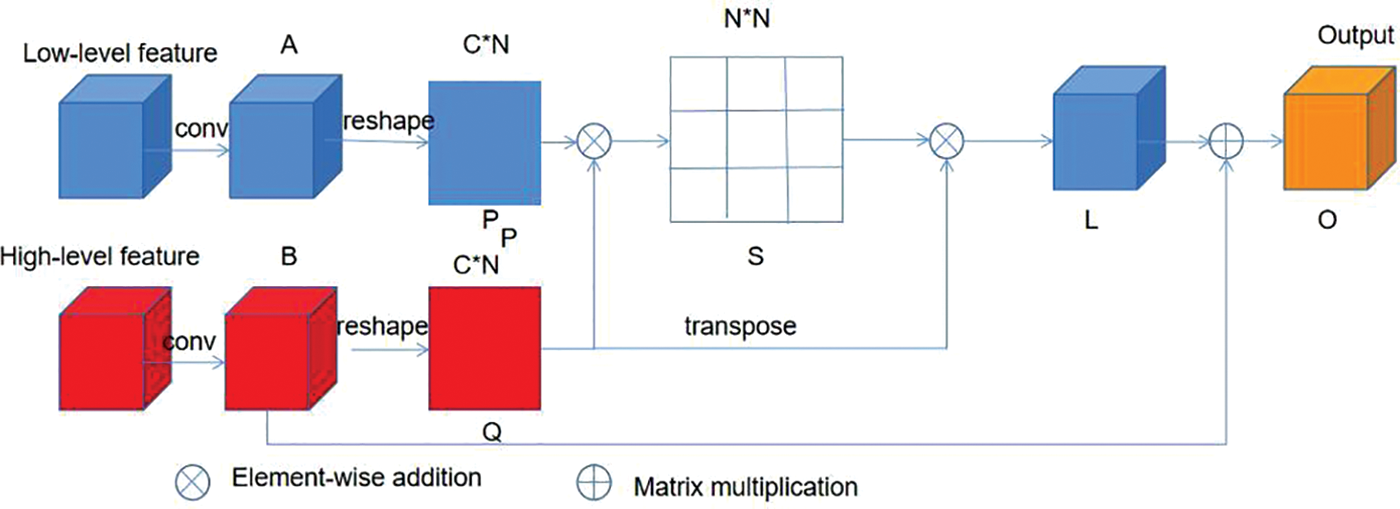
Figure 11: Multi-scale feature fusion module

Among α initialize to 0 and gradually learn to allocate more weights qi, represents the ith pixel in the low-dimensional feature maps, and Bj is the jth channel in the high-dimensional feature map. From (8), it can be inferred that each position of the final feature O is the weighted sum of all top-quality functions. Because shallow parts generate the last semantic features, they will contain rich semantic information [34].

3.4.2 Channel Attention Module

Shallow features contain a lot of semantic information. The feature graph of every channel will generate a specific feature map, and every feature map will significantly impact the final output. Through the channel attention module shown in Fig. 12, the consistency of feature mapping at each layer is enhanced by changing the feature weights of each channel [35]. CAM (Channel Attention Module) is to reweight each channel based on all elements of each feature map. First, the global average pooling layer is used to compress the feature map size and the number of feature channels [36]. Then, the corresponding weight vector is generated by the modified activation function (ReLU) and sigmoid function. Finally, the output feature map is generated by combining the matrix multiplication operation with the input feature map. Integrate the general information into the weight vector to ensure the reliability of feature mapping in turn [37].

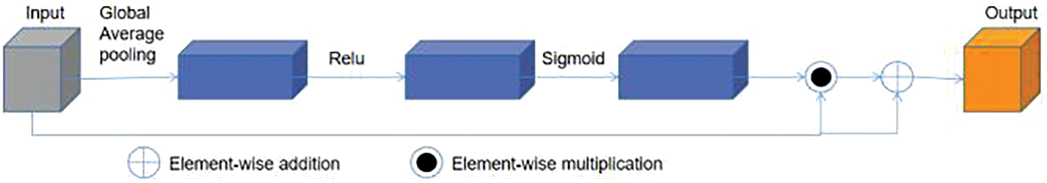
Figure 12: Channel attention module

3.4.3 Atrous Convolutional Spatial Pyramid Pooling

The Atrous Convolutional Spatial pyramid pooling (ASPP) incorporates Aperture Convolutions into SPP. Atrous convolutional can systematically aggregate image feature information at different scales and levels without losing resolution [38].

The basic principle of atrous convolution is shown in formula (9):

y[i]=∑kx[i+r∗k]w[k](9)

In Eq. (9), i is the coordinates of each element in the two-dimensional matrix, r is the expansion rate of the atrous convolution, and k is the dimension of the convolution kernel [39]. The ordinary convolution can be viewed as an atrous convolution with a rate of expansion of 1.

For standard convolution operations, the sliding step size of the convolution kernel is 1, which can be divided into three situations [40]:

That is, when downsampling is performed while convolution is being performed, the dimension of the convolutional feature map will decline;

1. Indicating a convolution with an average step size of 1;

2. As the feature map is pooled, the dimension of the feature map will increase.

The atrous convolution fills in between the blank elements. It ignores the part or leaves the input unchanged, adding the weight of the convolution kernel parameter to 0, thereby expanding the acceptance domain, convolving with a value more excellent than one can achieve the same effect. However, downsampling will be performed simultaneously with the convolution, which will reduce the feature map’s size and is unsuitable for use [41].

Assuming that the atrous fraction of the atrous convolution is r and the dimension of the convolution kernel is k, the extent F of the receptive field obtained is:

F=(r−1)∗(k−1)+k(10)

The structure of the atrous convolutional spatial pyramid pooling is shown in Fig. 13. Compared with SPP, an empty convolution is inserted in front of each parallel pooling window to increase the extraction range of image features. The similar atrous convolution layers have four different expansion rates to extract feature information at different levels and scales [42].

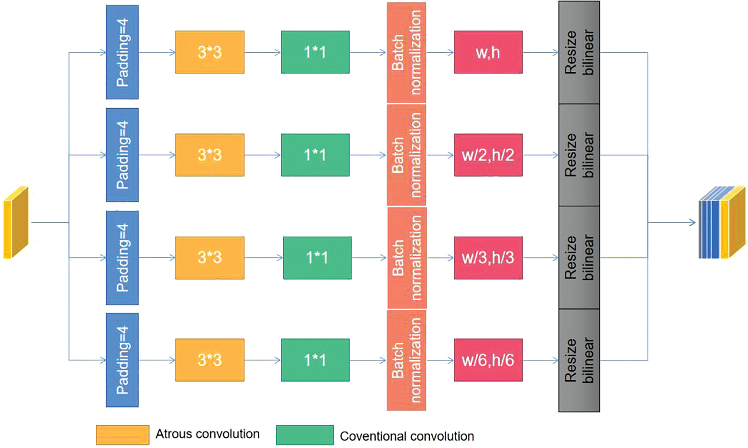
Figure 13: Structural diagram of ASPP

3.4.4 Construction of a GCNN Model for Atrous Convolutional Pyramid

Based on the traditional CNN model, multi-scale feature modules and attention channels are added to form an 8-layer convolutional neural network, including six convolutional layers and two fully connected layers. Maxpool is used for all pooling layers. In this paper, the improved ResNet network based on MSFFM-CAM-ASPP is named GCNN. An atrous convolution pyramid is introduced behind the sixth pooling layer to enlarge the field of view and enhance the feature extraction capability of the network. After pooling, the first five pooling layers are connected to the fusion layer by multi-scale feature modules, and the data features of different levels are extracted. Finally, the data is fused with the components extracted by ASPP. The network structure is shown in Fig. 14.

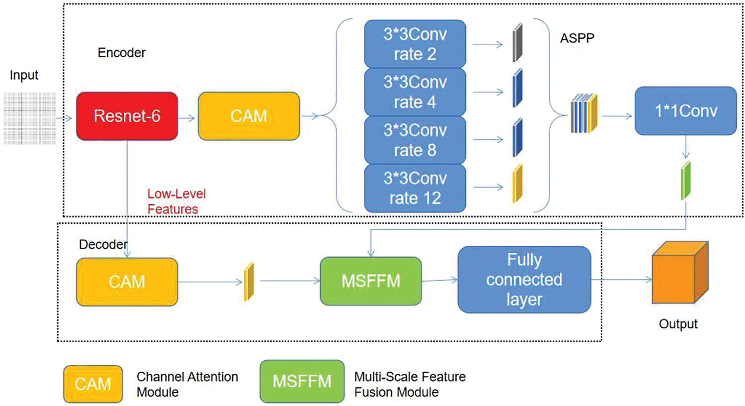
Figure 14: GCNN neural network structure

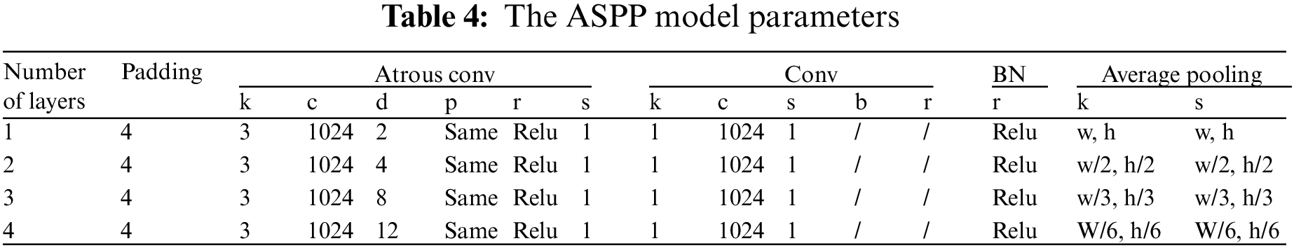
The four-layer ASPP adopts an average pooling layer. Although the highest pooling layer is standard, it can only output a maximum value and is unsuitable for GCNN networks with added atrous convolutional kernels. At each level of ASPP, feature maps with dimensions of (w, h) (w for width, h for height) are equally divided. For example, if it is divided into four modules, the dimension of every module will be (w/2, h/2); If it were divided into nine modules, the Measurement of every module would be (w/3, h/3); If it were divided into 36 modules, the dimension of every module would be (w/6, h/6). This article divides the four-layer feature maps into 1, 4, 9, and 36 modules, respectively, so that 50 sub-regions can be obtained and 50 different sets of image features can be extracted. These features are fused with the feature maps obtained from the first six convolutional layers through jump connections.

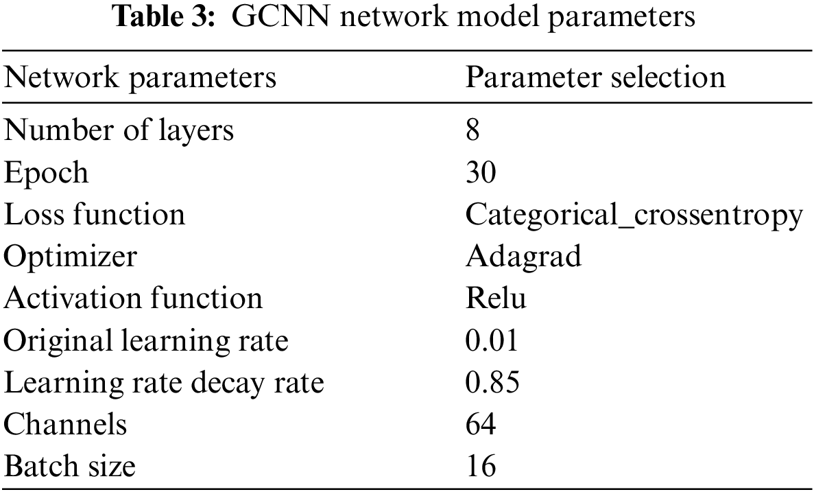
Every layer of ASPP in Fig. 14 has an atrous convolutional kernel, and the dimensions of the convolutional kernel are set to 3 × 3. Table 3 shows the parameters of the four-layer ASPP. Atrous convolutional kernels with high expansion rates will lose feature information, affect network accuracy, and affect the accuracy of the network. Therefore, using atrous convolutional kernels with low expansion rates to segment feature maps is common.

3.5 Parameter Configuration of the GCNN Model

GCNN network parameters are the optimal hyperparameters determined by the grid search method. The parameters are set reasonably, and the diagnostic accuracy of different faults is close to the maximum accuracy allowed by the theory.

This article adopts a step decay learning rate, and the selected decay learning rate function is:

k=k0∗a[nm](11)

Among them, k0 is the learning rate at the beginning of GCNN training; a is the attenuation coefficient of GCNN; n indicates how many rounds GCNN has trained so far; m is a constant applied to adjust the variation of GCNN learning rate; [nm] stands for rounding; k stands for the current learning rate of GCNN.

The initial learning rate is 0.01, the attenuation coefficient a is 0.85, and 30 rounds of training with a m of 5 can result in faster and better training results. The learning rate of GCNN during the exercise is shown in Fig. 15 [43]:

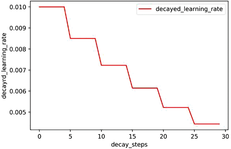
Figure 15: Step attendee’s learning rate

GCNN adopts the cross entropy that can be adopted to estimate the contrast between the theoretical value and the actual value to evaluate its loss function. The smaller the cross entropy value is, the closer the two probability distributions are, and it is described as formula (12) [44]:

C=−1n∑x[y∗lna+(1−y)∗ln(1−a)](12)

In formula (12), x stands for the sample, n stands for the total amount of models, y stands for the theoretical value, and it stands for the actual value.

The other model parameters in GCNN, except for ASPP, are shown in Table 3, and the model parameters of ASPP are shown in Table 4, where k is the size of the ordinary convolution kernel, c is the number of characteristic output channels, d is the expansion rate of cavity convolution kernel, p is the filling mode, r is the type of activation function, and b is the offset.

4  Results

4.1 GCNN Training Results and Comparison Experiment

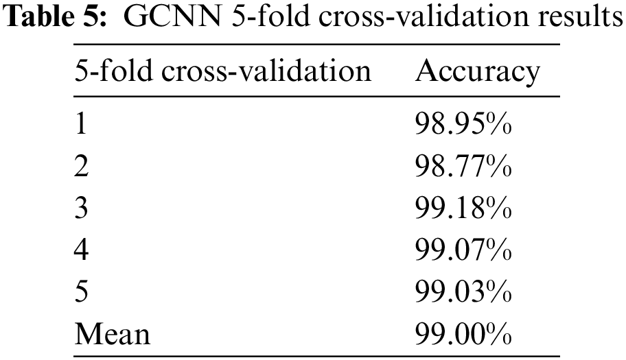
The produced data set was imported into the built GCNN model for training. The training results are shown in Fig. 16. The accuracy of the test set is 99.08%, and the loss function is 0.0035. The diagnostic accuracy of De25, De50, He, Se10, and Se20 motors is 99.80%, 99.60%, 99.70%, 98.10%, and 98.20%, respectively, which has high diagnostic accuracy. In addition, cross-validation was used to repeat the experiment many times to enhance the reliability of training results and avoid the interference of random factors on experimental results. After many experiments, it is found that the average accuracy of the five-fold cross-validation is the highest. The verification results of GCNN are shown in Table 5. The difference between the average and experimental results obtained by random segmentation data is only 0.08%, which can fully prove the reliability of the experimental results.

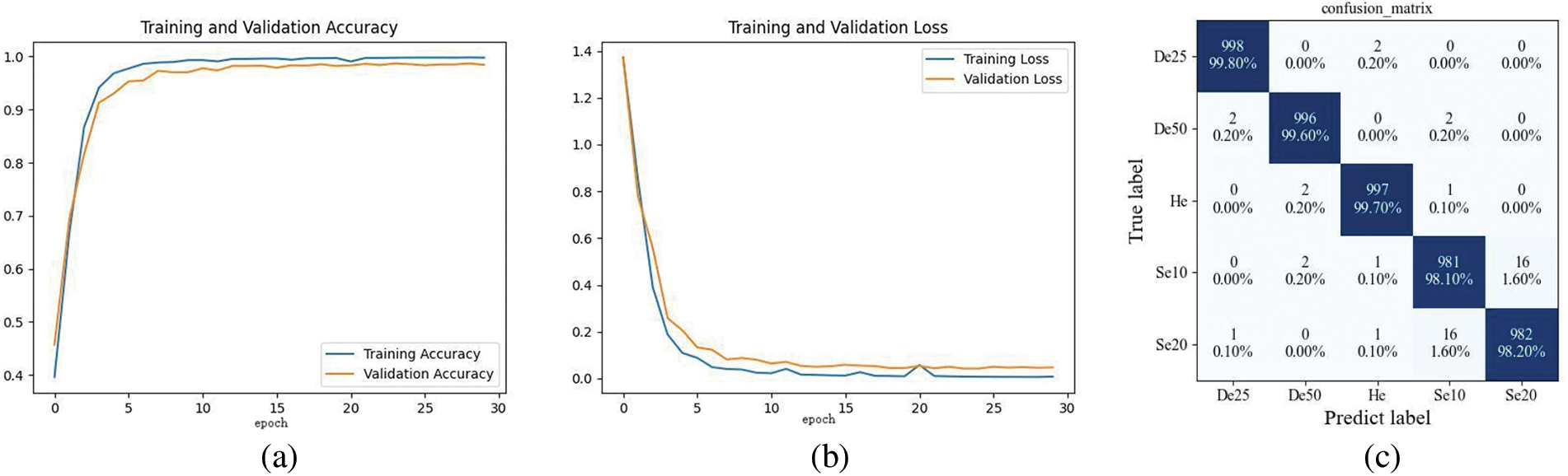
Figure 16: GCNN model test results: (a) Accuracy curve; (b) Loss graph; (c) Test result confusion matrix

To demonstrate the advantage of the GCNN, this paper conducts comparison experiments with MCNN [27], Bi-LSTM [45], DBN [46], and RNN [47], respectively, and the experimental results are shown in Fig. 17. The optimal hyperparameters of other comparison algorithms are determined by the grid search method, the parameters are set reasonably, and the diagnostic accuracy of different faults is close to the maximum accuracy allowed by the theory. The data set used is the same data set as GCNN, and both are self-made data sets. It can be seen that the accuracy rates of MCNN, Bi-LSTM, DBN, and RNN on the test set are 97.96%, 90.11%, 94.42%, and 91.78%, respectively, which are much lower than 99.00% of GCNN; the loss functions of the four comparison algorithms are 0.099, 0.242, 0.168, and 0.231, respectively, which are higher than that of GCNN. The comparison experiments thoroughly verify the superiority of GCNN.

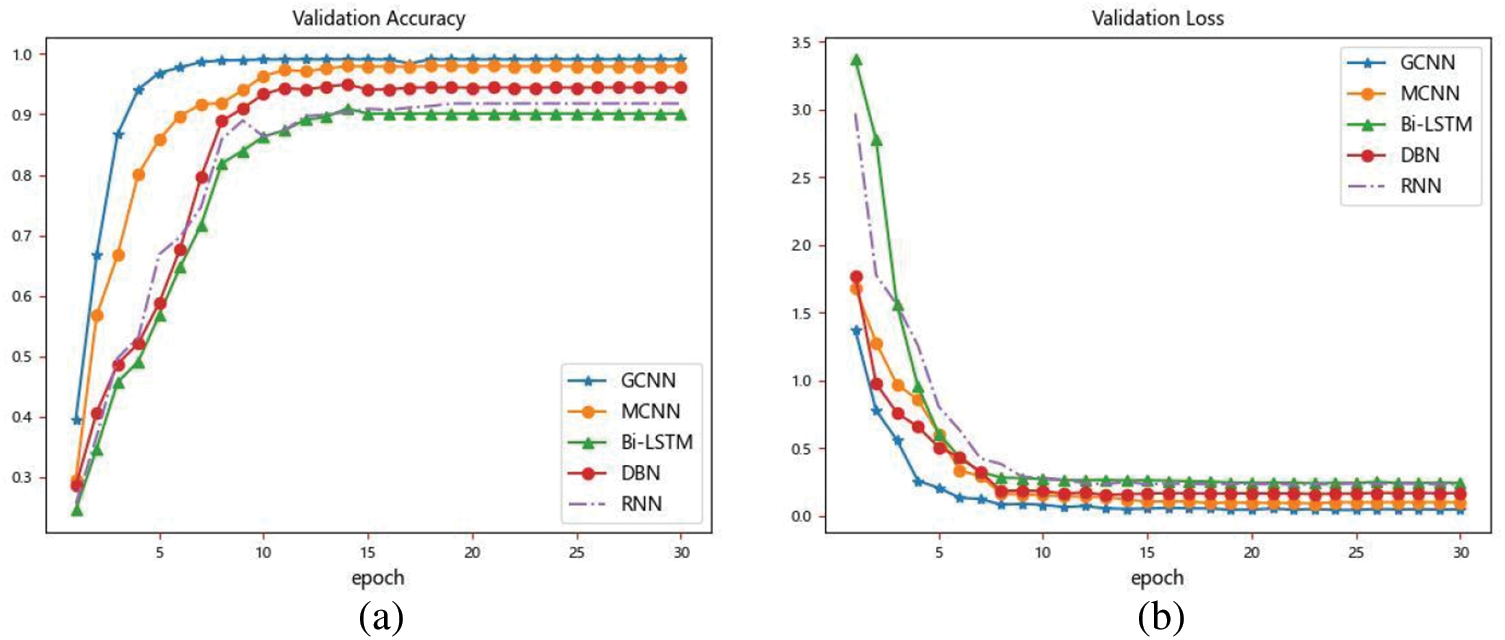
Figure 17: The result of comparison experiments: (a) Accuracy curve; (b) Loss graph

4.2 Noise Interference Experiment

In order to verify the anti-interference ability and robustness of the model proposed in this paper against noise, Gaussian noise, black pepper and salt noise, white pepper and salt noise, and black pepper and salt mixed noise with white pepper and salt were added to the self-made data set, respectively. The gray images after adding noise are shown in Figs. 18–21. After adding noise, different network fault diagnosis accuracy rates are shown in Table 6, and the parameters of each network for comparison experiment are determined as the optimal parameters by the grid search method.

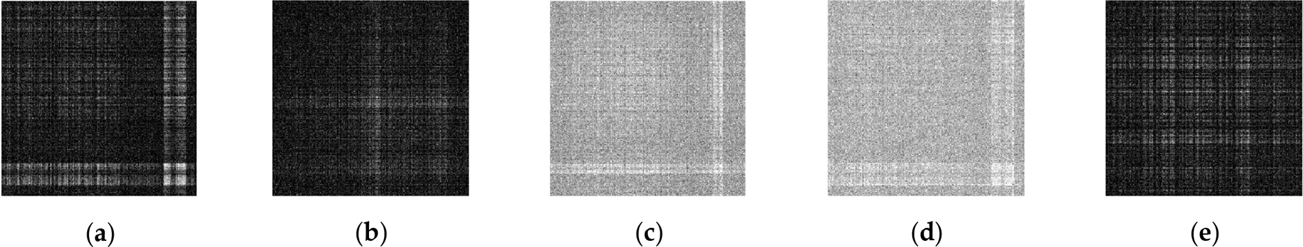
Figure 18: Grayscale images of different faults after adding Gaussian noise (load is 0 N.m): (a) De25; (b) De50; (c) Normal; (d) Se10; (e) Se20

Figure 19: Grayscale images of different faults after adding Black salt-and-pepper noise (load is 0 N.m): (a) De25; (b) De50; (c) Normal; (d) Se10; (e) Se20

Figure 20: Grayscale images of different faults after adding White salt-and-pepper noise (load is 0 N.m): (a) De25; (b) De50; (c) Normal; (d) Se10; (e) Se20

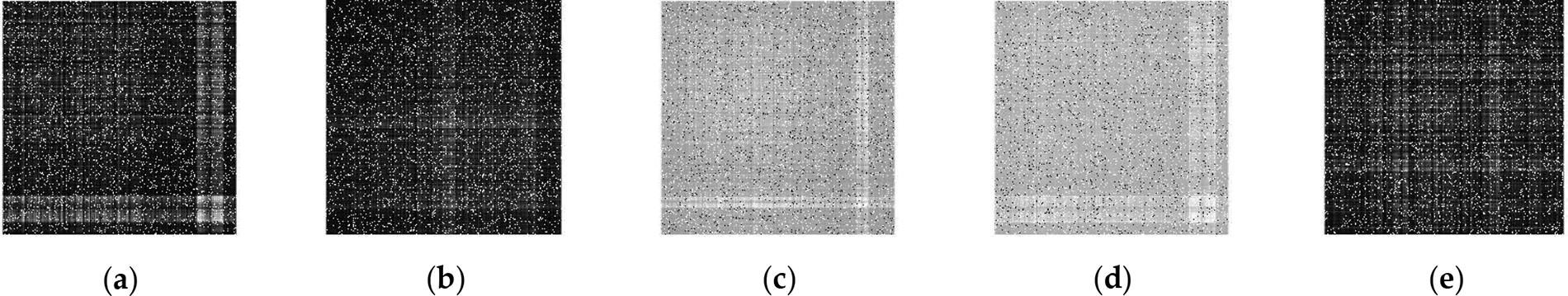
Figure 21: Grayscale images of different faults after adding Black and white salt-and-pepper noise (load is 0 N.m): (a) De25; (b) De50; (c) Normal; (d) Se10; (e) Se20

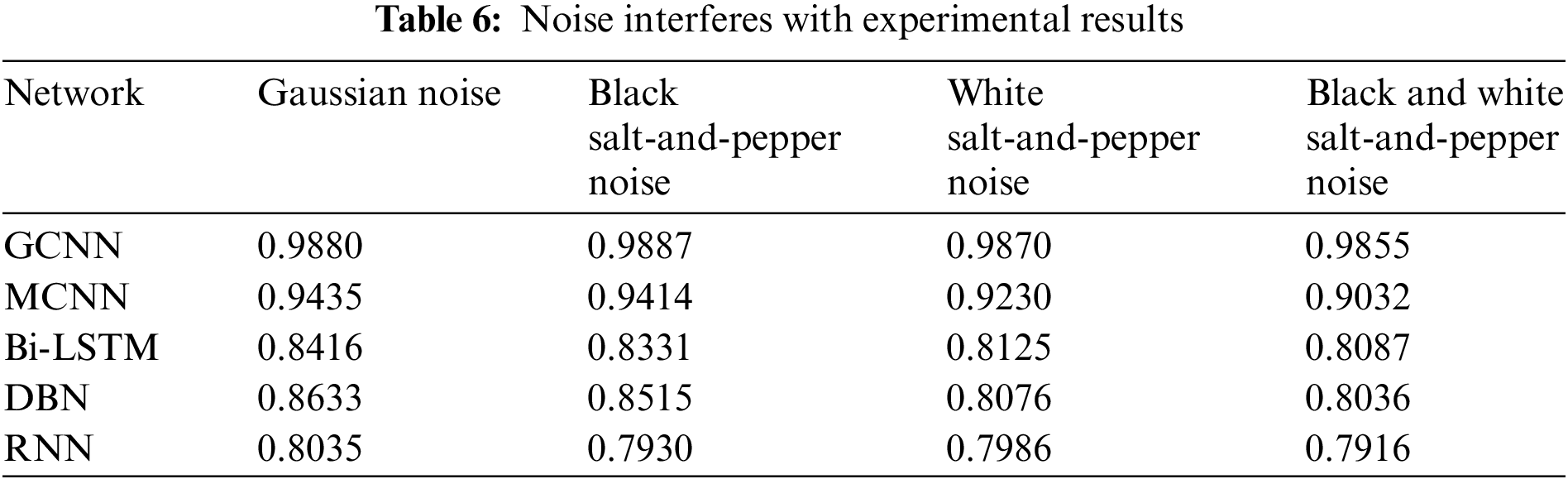
It can be seen from the results of noise interference experiments that the fault diagnosis accuracy of the proposed GCNN network for different types of permanent magnet synchronous motors has not changed much in the face of noise interference such as Gaussian noise, black pepper and salt noise, white pepper and salt noise, black and white pepper, and salt noise, and is always maintained within 0.5%. The ability of anti-noise interference and robustness are obviously better than the other four networks.

4.3 Interpretability Analysis of Fault Characteristics

4.3.1 The Visualization Technique of CNN—Grad-CAM

Different channels of the convolutional neural network convolutional layer can extract other fault features from images, and these fault features are related to PMSM fault types to some extent [48]. The correlation between fault characteristics and fault types of different channels is also distinct, so assigning different weights to these fault characteristics is necessary. However, obtaining the weight parameters of output features of various media from the convolutional neural network is problematic, resulting in the need for more interpretability of the mapping relationship established by deep learning [49].

To solve this problem, the Grad-CAM visualization analysis method is adopted in this paper to calculate the weight k of each channel, and the feature map of each channel is superimposed with the weight k to generate the thermal activation map [50]. The intensity of pixel color in the thermal activation map corresponds to the correlation degree of features, and the closer the pixel color is to the warm color, The more significant the activation intensity of features, the higher the degree of correlation, which can directly reflect the basis for CNN to judge fault characteristics [51].

The principle formula of Grad-CAM is shown in formulas (13) and (14):

αk=1Z∑i∈p∑j∈qδlδAijk(13)

LGrad−cam=∑k|αk|Ak(14)

Type of αk said the weight of the K-th channel, Aijk as the K-th channel output characteristic figure, Ak in the element value of coordinates (i, j), p and q respectively extraordinary clinic figure the length and width, Z=p∗q and LGrad−cam is the Grad-CAM [52].

4.3.2 Method of Determining Fault Characteristics

The PMSM fault diagnosis method based on Grad-CAM is divided into two stages: the selection of the thermal map and the determination of the original data corresponding to the thermal map. The specific implementation steps are described as follows.

Selection of heat map: The time domain signals of PMSM of different fault types obtained by co-simulation have 8000 data points, and the bilateral spectrum diagram generated after FFT transformation also has 8000 data points, which are evenly distributed on the horizontal axis of 32 kHz. Since the bilateral spectrum is axisymmetric, only the half spectrum composed of the first 4000 data points can be analyzed. The gray image based on the autocorrelation matrix takes 500 data points every 30 points to upgrade the dimension, so studying every heat map is unnecessary. Theoretically, all the data points on the single side spectral diagram can be covered by analyzing the Grad-CAM of Nos. 1, 17, 33, 49, 65, 81, 97, 113, and 116 gray images of demagnetization fault and eccentric fault.

Determine the raw data corresponding to the heat map: Since each gray image is dimensionally upgraded from 500 data points, the gray image is strictly diagonal symmetric, and the pixel points in each row and column reflect the intensity of the corresponding data points in the original data. Therefore, the corresponding pixel points in the unilateral spectrum can be found by analyzing the pixels in the warm color region in the thermal map. Thus, the fault characteristics of demagnetization and eccentricity of PMSM are determined.

4.4 Fault Characteristics of Demagnetization and Static Eccentricity of PMSM

Grad-CAM of Nos. 1, 17, 33, 49, 65, 81, 97, 113, 116 gray images of 25% and 50% demagnetization faults were selected for analysis. The Grad-CAM is shown in Figs. 22 and 23.

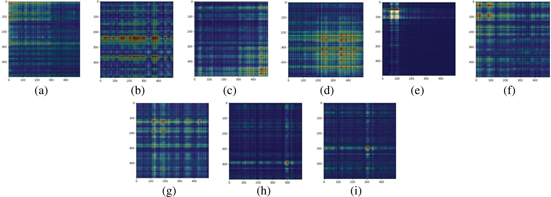
Figure 22: Grad-CAM corresponding to different gray level images of 25% demagnetization fault: (a) No. 1; (b) No. 17; (c) No. 33; (d) No. 49; (e) No. 65; (f) No. 81; (g) No. 97; (h) No. 113; (i) No. 116

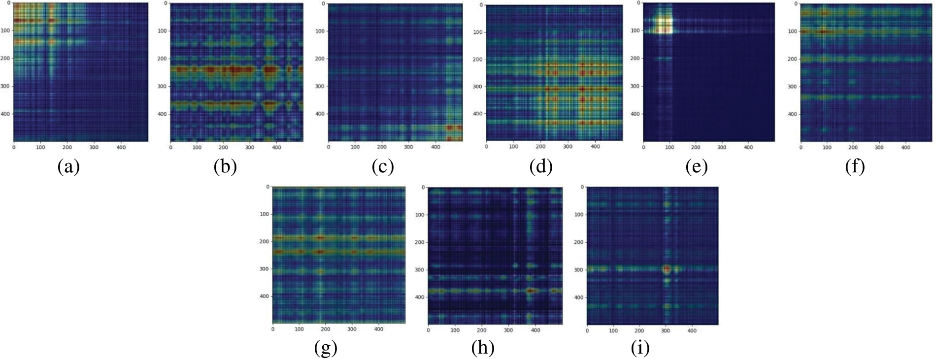
Figure 23: Grad-CAM corresponding to different gray level images of 50% demagnetization fault: (a) No. 1; (b) No. 17; (c) No. 33; (d) No. 49; (e) No. 65; (f) No. 81; (g) No. 97; (h) No. 113; (i) No. 116

The analysis of the Grad-CAM of 25% demagnetization and 50%PMSM gray image shows that the fault characteristics of demagnetization faults of different degrees are the same. There are 16 fault characteristics of demagnetization faults of PMSM. They are 140, 280, 440 Hz, 2.88, 3.44, 5.72, 6.68, 7.12, 7.48, 8, 9.68, 10, 12, 12.32, 12.64, 14.96 kHz; It is marked on the spectrum diagram of De25 and De50 fault PMSM, as shown in Fig. 24.

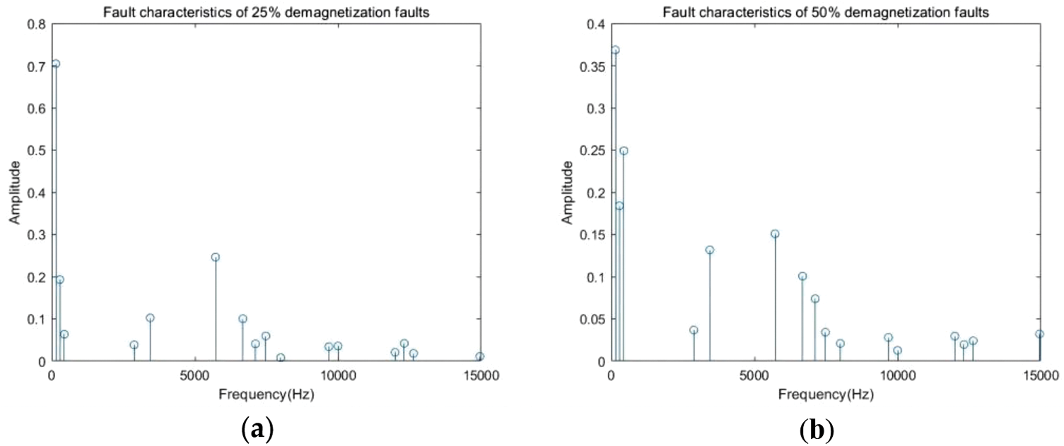
Figure 24: Fault characteristics corresponding to different demagnetizing faults: (a) De25; (b) De50

Similarly, Grad-CAM of Nos. 1, 17, 33, 49, 65, 81, 97, 113, and 116 gray images with 10% and 20% static eccentricity faults are analyzed. The gradient-type activation thermal maps (Grad-CAM) are shown in Figs. 25 and 26.

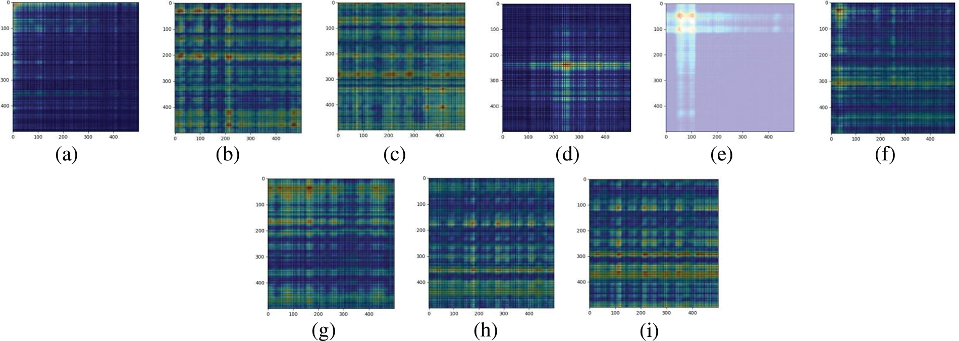
Figure 25: Grad-CAM corresponding to different gray level images of 10% static eccentricity fault: (a) No. 1; (b) No. 17; (c) No. 33; (d) No. 49; (e) No. 65; (f) No. 81; (g) No. 97; (h) No. 113; (i) No. 116

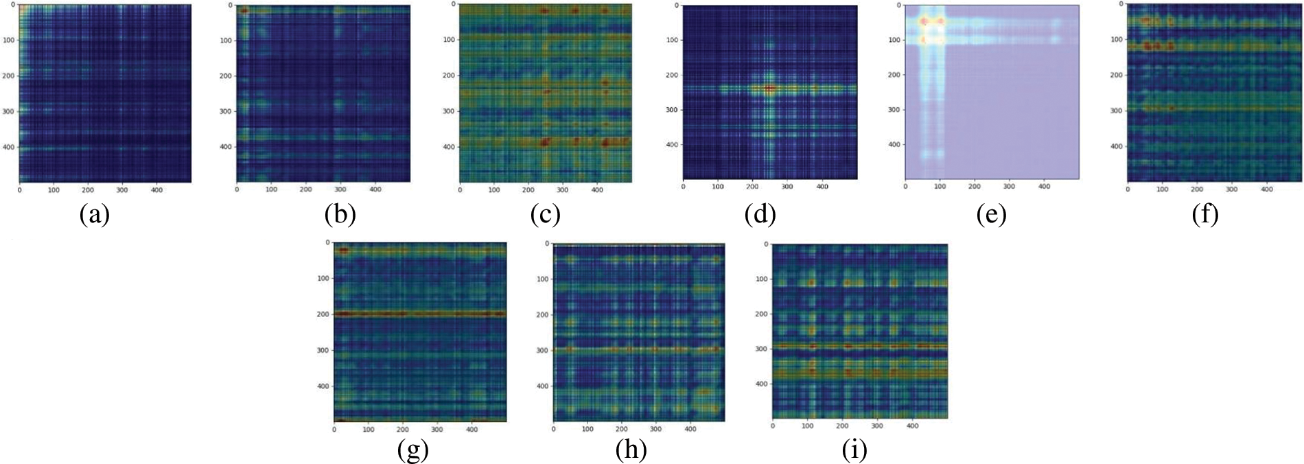
Figure 26: Grad-CAM corresponding to different gray level images of 20% static eccentricity fault: (a) No. 1; (b) No. 17; (c) No. 33; (d) No. 49; (e) No. 65; (f) No. 81; (g) No. 97; (h) No. 113; (i) No. 116

Through the analysis of the Grad-CAM thermal map, it can be found that there are 21 fault features in Se10, were 180 Hz, 2, 3.04, 3.84, 4.16, 4.64, 4.96, 5.44, 5.76, 6.76, 8, 9.8, 10.88, 11.72, 12.24, 13.32, 14.16, 14.64, 14.88, 15.24, 15.72 kHz, it is marked on the PMSM spectrum diagram of Se10 and Se20 faults, as shown in Fig. 27.

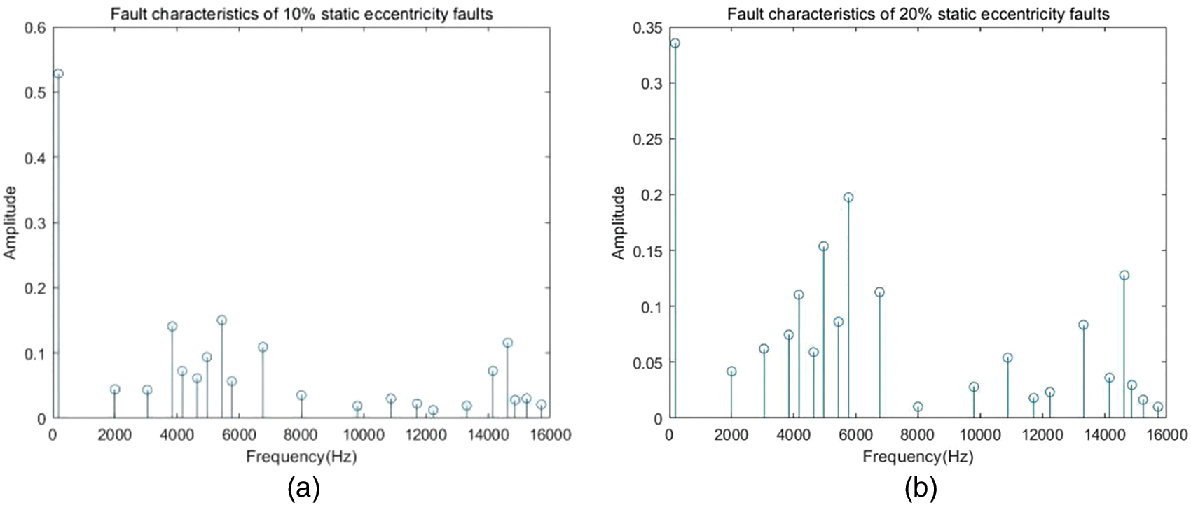
Figure 27: Fault characteristics corresponding to different demagnetizing faults: (a) Se10; (b) Se20

5  Discussion

In this paper, through the co-simulation of AltairFlux and MATLAB, the time domain signals of stator current in PMSM under different degrees of demagnetization and eccentricity fault are obtained. Then the frequency domain signals of the stator current are received by FFT. Then, it is transformed into a gray image by an image conversion method based on an autocorrelation matrix, and the data set is made. In Resnet-8, a multi-scale feature fusion module is constructed to extract image features of different levels, and the attention mechanism module is introduced to improve the feature extraction ability of CNN further. An ASPP is added in series at the end of CNN, and the sensitivity field of CNN is increased by hollow convolution. Its accuracy on the test set is 99.08%. In addition, given the defect that the traditional data-driven fault diagnosis method is unable to make interpretative analysis, this paper introduces Grad-CAM for interpretative analysis of different degrees of eccentricity and demagnetization faults, finds out their fault characteristics, and marks them on the spectrum diagram. However, the interpretative analysis method based on Grad-CAM proposed in this paper can only determine the general range of the symptoms and cannot accurately locate the fault characteristics. A plan can be found to locate different fault characteristics in the following research accurately.

The experimental data in this paper are all co-simulated by Flux and MATLAB and do not involve complex scenes with multiple heterogeneous targets. However, our research team is purchasing the faulty motor and the corresponding drive platform and plans to simulate better the operation state of permanent magnet synchronous motor on new energy vehicles in future research.

6  Conclusions

This paper presents a fault diagnosis method based on improved ResNet9 and Grad-CAM. It is used to diagnose demagnetization and eccentricity faults of permanent magnet synchronous motors and determine their fault frequency. The data set used in this paper was obtained by joint simulation of Flux and MATLAB. The data set contained 7,500 fault images of different types of permanent magnet synchronous motors, the specific parameters shown in Table 2. The overall accuracy of the improved ResNet9 network fault diagnosis results proposed in this paper is 99.00%, which has higher diagnostic accuracy than other traditional deep learning algorithms and has good robustness in the face of different noise interference. In addition, the “black box” problem in neural network fault diagnosis is solved using Grad-CAM. The demagnetization and eccentricity faults of permanent magnet synchronous motors are analyzed, and their fault characteristics are determined.

Acknowledgement: The authors would like to thank the Scientific Committee of the National Nature Foundation of China and the Scientific Committee of the Guizhou Provincial Nature Foundation for their funding of this research project.

Funding Statement: This study was funded by National Natural Science Foundation of China (Grant Numbers 51867006, 51867007) and the Natural Science and Technology Foundation of the Guizhou Province, China (Grant Numbers [2018]5781, [2018]1029).

Author Contributions: Study conception and design: Youming Guo, Qinmu Wu; data collection: Youming Guo; analysis and interpretation of results: Youming Guo; draft manuscript preparation: Youming Guo, Qinmu Wu. All authors reviewed the results and approved the final version of the manuscript.

Availability of Data and Materials: The data using in this paper are collected simulation experiment, and the modeling method is showed clearly in paper.

Conflicts of Interest: The authors declare that they have no conflicts of interest to report regarding the present study.

References

1. A. G. Espinosa, J. A. Rosero and J. Cusido, “Fault detection by means of Hilbert–Huang transform of the stator current in a PMSM with demagnetization,” IEEE Transactions on Energy Conversion, vol. 25, no. 2, pp. 312–318, 2010. [Google Scholar]

2. J. D. McFarland and T. M. Jahns, “Investigation of the rotor demagnetization characteristics of interior PM synchronous machines during fault conditions,” IEEE Transactions on Industry Applications, vol. 50, no. 4, pp. 2768–2775, 2014. [Google Scholar]

3. S. K. Kommuri, M. Defoort and H. R. Karimi, “A robust observer-based sensor fault-tolerant control for PMSM in electric vehicles,” IEEE Transactions on Industrial Electronics, vol. 63, no. 12, pp. 7671–7681, 2016. [Google Scholar]

4. Y. Gao, R. Qu and D. Li, “Improved hybrid method to calculate inductances of permanent magnet synchronous machines with skewed stators based on winding function theory,” Chinese Journal of Electrical Engineering, vol. 2, no. 1, pp. 52–61, 2016. [Google Scholar]

5. W. Sun, J. Hang and S. Ding, “Electromagnetic parameters analysis of inter-turn short circuit fault in DTP-PMSM based on finite element method,” in Int. Conf. on Power Electronics Systems and Applications (PESA), Hong Kong, China, pp. 1–4, 2020. [Google Scholar]

6. S. Fu, J. Qiu and L. Chen, “Adaptive fuzzy observer-based fault estimation for a class of nonlinear stochastic hybrid systems,” IEEE Transactions on Fuzzy Systems, vol. 30, no. 1, pp. 39–51, 2020. [Google Scholar]

7. M. Eftekhari, M. Moallem and S. Sadri, “Online detection of Induction motor’s stator winding short-circuit faults,” IEEE Systems Journal, vol. 8, no. 4, pp. 1272–1282, 2014. [Google Scholar]

8. H. Keskes and A. Braham, “Recursive undecimated wavelet packet transform and DAG SVM for Induction motor diagnosis,” IEEE Transactions on Industrial Informatics, vol. 11, no. 5, pp. 1059–1066, 2015. [Google Scholar]

9. N. P. Nguyen, N. X. Mung and L. N. N. Thanh Ha, “Finite-time attitude fault tolerant control of quadcopter system via neural networks,” Mathematics, vol. 8, no. 9, pp. 1541, 2020. [Google Scholar]

10. N. P. Nguyen, N. X. Mung and H. L. N. N. Thanh, “Adaptive sliding mode control for attitude and altitude system of a quadcopter UAV via the neural network,” IEEE Access, vol. 9, pp. 40076–40085, 2021. [Google Scholar]

11. J. Zhang, J. Liu and Z. Wang, “Convolutional neural network for crowd counting on metro platforms,” Symmetry, vol. 13, no. 4, pp. 703, 2021. [Google Scholar]

12. S. M. M. Hossain, K. Deb and P. K. Dhar, “Plant leaf disease recognition using depth-wise separable convolution-based models,” Symmetry, vol. 13, no. 3, pp. 511, 2021. [Google Scholar]

13. P. K. Kankar, S. C. Sharma and S. P. Harsha, “Fault diagnosis of ball bearings using machine learning methods,” Expert Systems with Applications, vol. 38, no. 3, pp. 1876–1886, 2011. [Google Scholar]

14. R. Liu, G. Meng and B. Yang, “Dislocated time series convolutional neural architecture: An intelligent fault diagnosis approach for an electric machine,” IEEE Transactions on Industrial Informatics, vol. 13, no. 3, pp. 1310–1320, 2016. [Google Scholar]

15. W. Zhang, C. Li and G. Peng, “A deep convolutional neural network with new training methods for bearing fault diagnosis under noisy environment and different working load,” Mechanical Systems and Signal Processing, vol. 100, no. 6, pp. 439–453, 2018. [Google Scholar]

16. I. H. Kao, W. J. Wang and Y. H. Lai, “Analysis of permanent magnet synchronous motor fault diagnosis based on learning,” IEEE Transactions on Instrumentation and Measurement, vol. 68, no. 2, pp. 310–324, 2018. [Google Scholar]

17. A. Jawaharlalnehru, T. Sambandham, V. Sekar, D. Ravikumar, V. Loganathan et al., “Target object detection from unmanned aerial vehicle (UAV) images based on improved YOLO algorithm,” Electronics, vol. 11, pp. 2343, 2023. [Google Scholar]

18. M. Anul Haq, “CNN based automated weed detection system using UAV imagery,” Computer Systems Science and Engineering, vol. 42, no. 2, pp. 837–849, 2022. [Google Scholar]

19. M. Anul Haq, “CDLSTM: A novel model for climate change forecasting,” Computers, Materials & Continua, vol. 71, no. 2, pp. 2363–2381, 2022. [Google Scholar]

20. M. Anul Haq, “DCNNBT: A novel deep convolutional neural network-based brain tumor classification model,” Fractals, vol. 31, no. 6, pp. 2340102–2340128, 2023. [Google Scholar]

21. M. Anul Haq, “Implementation of CNN for plant identification using UAV imagery,” International Journal of Advanced Computer Science and Applications (IJACSA), vol. 14, no. 4, pp. 830–847, 2023. [Google Scholar]

22. I. H. Kao, W. J. Wang and Y. H. Lai, “Analysis of permanent magnet synchronous motor fault diagnosis based on learning,” IEEE Transactions on Instrumentation and Measurement, vol. 68, no. 2, pp. 310–324, 2019. [Google Scholar]

23. A. L. Rodriguez, L. Huang and P. Lombard, “Vibration analysis of a PMSM through FEM multiphysics simulation with experimental validation,” in Int. Conf. on Electrical Machines (ICEM), Hong Kong, China, pp. 2560–2566, 2020. [Google Scholar]

24. Y. Qin and X. Shi, “Fault diagnosis method for rolling bearings based on two-channel CNN under unbalanced datasets,” Applied Sciences, vol. 12, pp. 8474, 2022. [Google Scholar]

25. C. Fu, X. Gui and F. Akter, “Discrete fourier transform (DFT)-based computational intelligence model for urban carbon emission and economic growth,” Mathematical Problems in Engineering, vol. 2022, pp. 1–10, 2022. [Google Scholar]

26. A. Abbassi, R. B. Mehrez and R. Abbassi, “Improved off-grid wind/photovoltaic/hybrid energy storage system based on a new framework of Moth-Flame optimization algorithm,” International Journal of Energy Research, vol. 46, no. 5, pp. 6711–6729, 2022. [Google Scholar]

27. Z. Li, Q. Wu and S. Yang, “Diagnosis of rotor demagnetization and eccentricity faults for PMSM based on deep CNN and image recognition,” Complex & Intelligent Systems, vol. 8, pp. 5469–5488, 2022. [Google Scholar]

28. O. Moutik, H. Sekkat, S. Tigani, A. Chehri, R. Saadane et al., “Convolutional neural networks or vision transformers: Who will win the race for action recognitions in visual data,” Sensors, vol. 23, no. 2, pp. 734, 2023. [Google Scholar] [PubMed]

29. A. Barua, M. U. Ahmed and S. Begum, “A systematic literature review on multimodal machine learning: Applications, challenges, gaps, and future directions,” IEEE Access, vol. 11, pp. 14804–14831, 2023. [Google Scholar]

30. Y. Yu, C. Wang, Q. Fu, R. Kou, F. Huang et al., “Techniques and challenges of image segmentation: A review,” Electronics, vol. 12, pp. 1199, 2023. [Google Scholar]

31. S. Deb and S. Sinha, “Comparative improvement of image segmentation performance with graph-based method over watershed transform image segmentation,” In: R. Natarajan (Ed.Distributed Computing and Internet Technology: ICDCIT, pp. 322–332, Cham, New York, NY, USA: Springer, 2014. [Google Scholar]

32. H. Wang and P. A. Yushkevich, “Guiding automatic segmentation with multiple manual segmentations,” in Int. Conf. on Medical Image Computing and Computer-Assisted Intervention, Berlin, Heidelberg, Germany, Springer, pp. 429–436, 2012. [Google Scholar]

33. N. Nikbakhsh and Y. Baleghi, “A new fast method of image segmentation fusion using maximum mutual information,” in Iranian Conf. on Electrical Engineering (ICEE), Yazd, Iran, pp. 1584–1588, 2019. [Google Scholar]

34. Z. Yan, H. Wang, Q. Ning and Y. Lu, “Robust image matching based on image feature and depth information fusion,” Machines, vol. 10, no. 6, pp. 456, 2022. [Google Scholar]

35. H. Lee and S. Cho, “Locally adaptive channel attention-based network for denoising images,” IEEE Access, vol. 8, pp. 34686–34695, 2020. [Google Scholar]

36. Y. Yang, X. Wang, B. Sun and Q. Zhao, “Channel expansion convolutional network for image classification,” IEEE Access, vol. 8, pp. 178414–178424, 2020. [Google Scholar]

37. S. Seong and J. Choi, “Semantic segmentation of urban buildings using a high-resolution network (HRNet) with channel and spatial attention gates,” Remote Sensing, vol. 13, pp. 3087, 2021. [Google Scholar]

38. M. H. Park, J. H. Cho and Y. T. Kim, “CNN model with multilayer ASPP and two-step cross-stage segmentation,” Machines, vol. 11, no. 2, pp. 126, 2023. [Google Scholar]

39. S. Q. Du, S. J. Tang, W. X. Wang, X. M. Li, Y. H. Lu et al., “PSCNET: Efficient RGB-D semantic segmentation parallel network based on spatial and channel attention,” Remote Sensing, vol. 1, pp. 129–136, 2022. [Google Scholar]

40. S. Wang, C. Hu, K. Cui, R. Wang, H. Mao et al., “Animal migration patterns extraction based on atrous-gated CNN deep learning model,” Remote Sensing, vol. 13, no. 24, pp. 4998, 2022. [Google Scholar]

41. M. Abdullah Alkhonaini, S. Ben Haj Hassine, M. Obayya, F. N. Al-Wesabi, A. Mustafa Hilal et al., “Detection of lung tumor using ASPP-Unet with a whale optimization algorithm,” Computers, Materials & Continua, vol. 72, no. 2, pp. 3511–3527, 2022. [Google Scholar]

42. Y. Li, Z. Cheng, C. Wang, J. Zhao and L. Huang, “RCCT-ASPPNet: Dual-encoder remote image segmentation based on transformer and ASPP,” Remote Sensing, vol. 15, no. 2, pp. 379, 2023. [Google Scholar]

43. B. Liu, Q. Wu, Z. Li and X. Chen, “Research on fault diagnosis of PMSM for electric vehicles based on multi-level feature fusion SPP network,” Symmetry, vol. 13, pp. 1844, 2021. [Google Scholar]

44. M. Javed Awan, M. S. Mohd Rahim, N. Salim, M. A. Mohammed, B. Garcia-Zapirain et al., “Efficient detection of knee anterior cruciate ligament from magnetic resonance imaging using deep learning approach,” Diagnostics, vol. 11, no. 1, pp. 105, 2021. [Google Scholar]

45. L. Chen, Z. Zhang and J. Cao, “A novel method of combining nonlinear frequency spectrum and deep learning for complex system fault diagnosis—ScienceDirect,” Measurement, vol. 151, pp. 107190, 2020. [Google Scholar]

46. T. Zhang, Z. Li and Z. Deng, “Hybrid data fusion DBN for intelligent fault diagnosis of vehicle reducers,” Sensors, vol. 19, no. 11, pp. 2504, 2019. [Google Scholar] [PubMed]

47. J. He, J. Lee and T. Song, “Recurrent neural network (RNN) for delay-tolerant repetition-coded (RC) indoor optical wireless communication systems,” Optics Letters, vol. 44, no. 15, pp. 3745–3748, 2019. [Google Scholar] [PubMed]

48. R. R. Selvaraju, M. Cogswell and A. Das, “Grad-CAM: Visual explanations from deep networks via gradient-based localization,” IEEE International Conference on Computer Vision, vol. 128, no. 2, pp. 336–359, 2020. [Google Scholar]

49. S. H. Wang, Y. Zhang, X. Cheng, X. Zhang and Y. Zhang, “PSSPNN: PatchShuffle stochastic pooling neural network for an explainable diagnosis of COVID-19 with multiple-way data augmentation,” Computational and Mathematical Methods in Medicine, vol. 2021, pp. 1–18, 2021. [Google Scholar]

50. A. Chattopadhay, A. Sarkar, P. Howlader and V. N. Balasubramanian, “Grad-CAM++: Generalized gradient-based visual explanations for deep convolutional networks,” in IEEE Winter Conf. on Applications of Computer Vision (WACV), Lake Tahoe, NV, USA, pp. 839–847, 2018. [Google Scholar]

51. R. R. Selvaraju, M. Cogswell, A. Das, R. Vedantam, D. Parikh et al., “Grad-CAM: Visual explanations from deep networks via gradient-based localization,” in IEEE Int. Conf. on Computer Vision (ICCVVenice, Venice, Italy, pp. 618–626, 2017. [Google Scholar]

52. S. Kolekar, S. Gite, B. Pradhan and A. Alamri, “Explainable AI in scene understanding for autonomous vehicles in unstructured traffic environments on Indian roads using the inception U-Net model with Grad-CAM visualization,” Sensors, vol. 22, no. 24, pp. 9677, 2022. [Google Scholar] [PubMed]