An Improved Whale Optimization Algorithm for Global Optimization and Realized Volatility Prediction

1  Introduction

The volatility of financial markets refers to the degree of volatility of the prices of financial assets, which serves as a crucial risk indicator. Realized Volatility (RV) has become one of the most commonly used volatility measures, which is widely employed to assess the Value at Risk (VaR) of investment portfolios and to determine the pricing of derivatives based on options. Consequently, the prediction of RV in financial markets has become a topic of great interest to both theoretical and practical communities.

Since RV has the characteristics of long memory and aggregation [1], the AutoRegressive Fractionally Integrated Moving Average (ARFIMA) [2] and the Heterogeneous Autoregressive Model (HAR) [3] that can capture these two characteristics have become the most widely used models for RV prediction. Autoregressive has become the most widely used model for RV prediction. The research of scholars using the ARFIMA model to capture the long memory of economic data started in the 1990s. Subsequently, scholars have conducted numerous improved studies on the limitations of ARFIMA in predicting RV. Andersen et al. [4], Giot et al. [5], and Degiannakis [6] all proposed improved models for the defects of the ARFIMA model. Furthermore, Zhou et al. [7] and Izzeldin et al. [8] both employed the ARFIMA model to study RV and demonstrated its excellent performance in RV prediction. Muller et al. proposed the HAR model in 1997. Later, Barndorff-Nielsen et al. [9] proposed improved versions of the HAR model. Meanwhile, numerous empirical studies have demonstrated the excellent performance of the HAR model in RV prediction [10,11]. However, the HAR and ARFIMA are both econometric models, and they both have the disadvantages of being limited to linear time series patterns and not providing accurate forecasts.

In recent years, artificial intelligence technology has led to the application of Long Short-Term Memory (LSTM) [12], which can capture nonlinear time series features, to the RV prediction problem. Maknickiene et al. [13] used LSTM to predict the rate of return of the exchange rate in 2012, and the results demonstrated that the prediction accuracy was improved compared to BP neural networks. Chen et al. [14] used the LSTM model to predict the returns of the Chinese stock markets in 2015. According to the results, the LSTM model’s prediction accuracy was better than the Stochastic Volatility (SV) model. In 2018, Kim et al. [15] used a mixture of Generalized AutoRegressive Conditional Heteroskedasticity (GARCH) and LSTM for predicting Korean stock market volatility and the results were impressive. Recently, scholars have also attempted to solve the RV prediction problem using LSTM. Hu et al. [16] proposed a combined model that integrates GARCH, LSTM, and Artificial Neural Network (ANN) in 2020 for predicting copper price volatility, which was more accurate than the other five models. The Complete Ensemble Empirical Mode Decomposition with Adaptive Noise (CEEMDAN) and LSTM model was applied by Lin et al. [17] in 2022 to predict the RV of the CSI300, S&P500, and STOCXX50 with good results, solving the problem of noise associated with RV time series. Chen et al. [18] used the Principal Component Analysis (PCA) and LSTM model to predict the volatility of Chinese and American stock index futures within the same year, and the experimental results were more accurate than the other seven models. The results suggest that PCA can improve the LSTM prediction performance by reducing attributes. While LSTM-based volatility prediction is highly accurate, the determination of the hyperparameters has always presented a challenge. In this paper, a meta-heuristic algorithm will be introduced to automate the process of hyperparameter optimization for LSTM.

The Genetic Algorithm (GA) [19] was first proposed and achieved great success in solving optimization problems in the 1960s, inspired by biological research. Metaheuristic algorithms have made significant progress since the 1980s. Kirkpatrick et al. [20] proposed the Simulated Annealing (SA) algorithm in 1982. Glover [21] proposed the Tabu Search Algorithm (TSA) in 1986. The Ant Colony Optimization (ACO) was proposed in 1992 by Dorigo [22]. In 1995, Venter et al. [23] proposed the concept of Particle Swarm Optimization (PSO). Storn et al. [24] introduced the Differential Evolution Algorithm (DE) in 1997. Many new meta-heuristic algorithms have been proposed in recent years, such as Monarch Butterfly Optimization (MBO) [25], Naked Mole-Rat Algorithm (NMR) [26], Moth Swarm Algorithm (MSA) [27], Harris Hawks Optimization (HHO) [28], Slime Mould Algorithm (SMA) [29], African Vultures Optimization Algorithm (AVOA) [30], Carnivorous Plant Algorithm (CPA) [31], and the Hunger Games Search (HGS) [32]. These algorithms have emerged as prominent representatives and have achieved significant success in solving optimization problems across various domains [33–39].

Mirjaliliab et al. [40] developed the Whale Optimization Algorithm (WOA) by mimicking humpback whales’ natural search, surround, and attack behaviors in 2016. The WOA algorithm has demonstrated its effectiveness in optimizing diverse problem domains, such as reservoir scheduling [41], workshop scheduling [42], rolling bearing fault diagnosis [43], turbine heat consumption prediction [44], and residue hydrogenation reaction kinetic model parameter optimization [45]. While the basic WOA algorithm is characterized by its simplicity and a limited number of parameters, it also has some shortcomings. First of all, the accuracy and speed of heuristic algorithms are directly affected by the quality of the initial population [46]. In general, the more diverse the initial population, the stronger the algorithm’s ability to perform global searches [47]. Random initialization of the original WOA does not produce an even distribution of the initial population throughout the whole search space, which affects the algorithm’s efficiency in solving problems. Additionally, the algorithm has a tendency to converge towards local extrema during the late stage of population evolution [48,49], which results in poor convergence accuracy.

There are two primary motivations for this study. First, this paper introduces a chaos mechanism and an opposition-based learning strategy to compensate for the limitations of the WOA. As of now, there are several works [50–55] that use chaos and opposition-based learning strategies to improve the WOA, among which literature [53] is the closest to the idea presented in this paper. However, the algorithm employed differs in two ways. In the first instance, the opposition-based learning operator is different. This paper adopts the classical opposition-based learning operator, similar to that described in the literature [52], while the partial-opposition-based learning operator, as discussed in the literature [53]. In the second instance, this paper introduces the Jumping rate (Jr) and discusses its parameter sensitivity, while in literature [53], Jr is fixed at 0.5. Second, to improving the accuracy of RV prediction, this paper proposes a prediction model based on the improved WOA-LSTM model. As of now, some applied research has been conducted on the improved LSTM model based on WOA [56–60], but this research takes a step further. In the first instance, the improved WOA algorithm has stronger optimization capabilities compared to the original WOA algorithm. In the second instance, the WOA-LSTM model is used to predict RV, thereby enhancing its usefulness.

In summary, this paper proposes an improved whale optimization algorithm called OLCHWOA, which utilizes chaos mechanisms and opposition-based learning techniques. In addition, an RV prediction model based on OLCHWOA-LSTM is developed. Through simulation experiments, this study has drawn several conclusions: (1) The experimental results of 38 test functions and three engineering design problems with constraints establish the superior performance of OLCHWOA with statistical significance when compared to the other five algorithms; (2) The RV prediction for the CSI 300 index in mainland China indicates that OLCHWOA-LSTM Models have a competitive advantage. As a result of our research, this paper has made two important contributions. First, the utilization of the chaos mechanism and opposition-based learning strategy improves the global search ability of the WOA algorithm and further advances related research. Additionally, this paper has developed an RV prediction model based on OLCHWOA-LSTM, which enhances the RV prediction method by introducing a novel approach for neural network-based RV prediction models.

In the remainder of the paper, the following sections will be discussed: Section 2 introduces the concept of OLCHWOA. The simulation experiment is presented in Section 3. Section 4 introduces the OLCHWOA-LSTM model and discusses its prediction performance on the RV of the CSI 300 dataset. Our conclusions are presented in Section 5.

2  Proposed Olchwoa Algorithm

2.1 Original WOA Algorithm

WOA is a novel heuristic optimization algorithm based on the mathematical modeling of the unique hunting method of humpback whales. In nature, humpback whales swim upward in a spiral position from the depths of the ocean and expel numerous bubbles of different sizes. Prey will be forced toward the center of the bubble net by the surrounding bubble net, at which point the whale opens its mouth and swallows the prey.

Since the initialized population of the WOA lacks a priori experience, it is assumed that the prey position is set as the global optimization, and other individual whales converge towards the prey position as a means of updating their own positions. The WOA algorithm for locating the optimal position relies on three mechanisms, which are described as follows.

2.1.1 Encirclement Hunting

By swimming towards the nearest whale in the group, the whales narrow the circle around their prey. The formula for updating whale positions is used in this process.

Xit+1=XPt−A∗D(1)

D=|C∗XPt−Xit|(2)

A=2a∗r1−a(3)

a=2−2∗t/tmax(4)

C=2∗r2(5)

where Xit+1 is the next position of the whale, Xpt is the current optimal whale, D is the encircling step. C is the effect of the distance between Xpt and individual Xit. When C > 1, the degree of influence is enhanced, and vice versa. The convergence factor, denoted as a, linearly decreases from 2 to 0 as the number of iterations increases. r1 and r2 represent random numbers within [0,1].

2.1.2 Spiral Hunting

The whales hunt by spiraling towards the prey’s position, and this can be expressed by the following formula:

Xit+1=D′∗ebl∗cos⁡(2πl)+XPt(6)

D′=|XPt−Xit|(7)

where D′ is the distance between Xit and Xpt, and the constant b determines the shape of the spiral. l is a random number within [−1,1], where l is −1 when whales are closest to the prey position, and l is 1 when whales are farthest from the prey position.

In addition, the whales swim around their prey while simultaneously conducting spiral hunting simultaneously. The probability Pr for an individual whale choosing encircling or spiral hunting is 50%. The behavior is as follows:

Xit+1={XPt−A∗D′,Pr<0.5D′∗ebl∗cos⁡(2πl)+XPt,Pr≥0.5(8)

2.1.3 Random Hunting

Additionally, whales can go on random hunts, which increases the search area for the whales. Following is the formula for this process:

 Xit+1=XRt−A∗D″(9)

D″=|C×XRt−Xit|(10)

where XRt is an individual whale randomly selected from the current population, D″ is the distance between Xit and XRt. A and C are defined in accordance with the definitions of the encircling hunting mechanism, with C controlling the distance between Xit and XRt.

When the parameter |A| < 1, the individual whale moves away from the random individual XRt to surround the prey, and then tends to the optimal individual Xpt. When the parameter |A| ≥ 1, the individual whale deviates from the prey position to search for a better prey. Therefore, the value of parameter A determines whether the individual whale adopts Eq. (1) or Eq. (9) to update its position. In light of the fact that parameter A is largely affected by the convergence factor a, a is an important consideration for the exploration and development of balanced algorithms.

2.2 Chaos Mechanism (CH)

The quality of the initial population has a significant impact on the optimization efficiency of metaheuristic algorithms [61]. Currently, the majority of metaheuristic algorithms employ random initialization to generate the initial population, which results in uneven distribution of the population across the solution space, reducing diversity and making the algorithm prone to premature convergence [62]. Chaos is a common nonlinear phenomenon distinguished by its non-repetition, ergodicity, and dynamism [63]. Using chaos mechanisms to generate the initial whale population, rather than random generation, can enhance the algorithm’s search efficiency during the search process [64], facilitating a faster exploration of the search space. Chaos mapping has been employed to address various optimization problems [65]. The logistic map is a simple and effective chaotic system whose expression is as follows:

chi+1=μ∗chi∗(1−chi),i={1,2,…,K}(11)

where μ is the control parameter, the value range is 0 < μ ≤ 4.0. When μ = 4, the logistic map is completely chaotic. K represents the number of iterations. ch1 is a random number within the interval [0, 1], while chi ≠ 0.25, 0.5 and 0.75.

Assuming that the initial whale population is composed of N individuals, the specific process of using the Logistic chaotic initialization operator to generate the initial whale population is as follows. The first individual is randomly generated within the upper and lower bounds. Then, Eq. (11) is used to iterate the first individual in order to obtain the remaining N-1 individuals. Finally, Eq. (12) is used to map variables to individual whales.

Xij=Xi,min_j+chji∗(Xi,max_j−Xi,min_j)(12)

where Xi, min_j, Xi, max_j define the upper and lower bounds of the j-th dimension of the i-th individual, respectively, Xij is the mapped whale individual.

Fig. 1 illustrates the distribution of a random population and a logistic chaotic population in a two-dimensional plane. Under different population sizes, it is found that the population generated by the logistic chaotic initialization operator exhibits better uniformity compared to the population generated by random initialization.

Figure 1: Comparison of two initialization methods in two-dimensional plane (a) Population size = 20, (b) Population size = 200

2.3 Opposition-Based Learning Strategy (OL)

Opposition-based learning (OBL) is an enhancement strategy introduced by Tizhoosh within the domain of swarm intelligence in 2005 [66]. At its core, OBL involves the simultaneous consideration of feasible solutions and their corresponding opposite solutions, selecting the best solutions for advancement to the next generation of the population. A significant limitation associated with random initialization is that when the current solution is considerably distant from the optimal solution, it may lead to prolonged search times or the algorithm getting stuck in local optima [67]. Interestingly, according to probability theory, solutions that are opposite to each other have a 50% probability of being closer to the optimal solution [68]. The integration of opposite solutions can result in significant enhancements in search efficiency while simultaneously reducing computational expenses [69].

The Opposition-based Learning strategy of this paper introduces two types of operators called the Opposition-based Initialization operator (OI) and the Elite Opposition-based Learning operator (EOL) to enhance WOA’s global search ability. Their detailed descriptions are as follows.

2.3.1 Opposition-Based Initialization Operator (OI)

As shown in Section 2.2, this paper introduces the chaotic initialization operator to generate the initial population, which ensures an even distribution of the initial population. To increase the search efficiency, this paper attempts to introduce an Opposition-based Initialization operator (OI) to further optimize the initial population.

The feasible solution is given by Xi = (xi1, xi2,…, xij), where xij∈ [lij, uij], i = 1, 2, …, N, j = 1, 2, …, D. Each dimension’s maximum and minimum values are represented by lij and uij. The opposite solution can be defined as Xi¯ = (x¯i1,x¯i2,…,x¯ij), which x¯ij is obtained by Eq. (13) as follows:

x¯ij=lij+uij−xij(13)

After obtaining the opposing population, the fitness values are compared between the original population and the opposing population. The individuals with the highest fitness values are then selected to be included in the initial population. Let the fitness function be f(.). The selection operator can be expressed as follows: The original population is compared with the opposite population in order to select the most suitable individuals for entry into the population.

Xi={X¯i , if f(X¯i)<f(Xi)Xi , else(14)

2.3.2 Elite Opposition-Based Learning Operator (EOL)

Based on the ideas of Wang et al. [70] and Zhou et al. [71], this paper proposes an Elite Opposition-based Learning operator (EOL). By introducing the Jumping rate (Jr), whales have a greater chance of jumping out of the local solutions, thereby improving the algorithm’s global search capability and thus improving the algorithm’s ability to search globally. According to this principle, if rand (0, 1) < Jr, the EOL will be executed. If not, the evolution will follow the original logic of WOA. There are two steps in the process of the EOL operator.

Step 1: if rand (0, 1) < Jr, then the elite opposition-based solution is generated according to Eq. (15) as X¯i=(x¯i,1,x¯i,2,…,x¯i,D).

X¯i,j=η(aj+bj)−xi,j(15)

where η is the generalized coefficient, η ∈ (0, 1), aj and bj are the upper and lower bounds.

aj=min(xi,j)(16)

bj=max(xi,j)(17)

Additionally, if the generated elite opposition-based solution crosses the boundary [aj, bj], it is reset according to Eq. (18).

x¯i,j=rand(aj, bj)(18)

Step 2: Compared with the current solution and the elite opposition-based solution, evaluate each solution’s fitness value, and the best individual will be selected to stay in the population according to Eq. (14). With the EOL operator, the population can be updated with the information contained in the current population, which will increase the convergence speed and the capabilities of WOA global exploration.

2.4 Olchwoa Algorithm

In the same way that other meta-heuristic algorithms encounter issues, WOA may also converge to a local optimum prematurely. An improved Whale Optimization Algorithm based on chaos mechanism and opposition-based learning (OLCHWOA) is designed to improve WOA’s global search capability and prevent a decrease in population diversity during later iterations.

During the initialization stage, the logistic chaotic initialization operator is used first to create a diverse population of high quality. Afterward, the opposite population is constructed using the OI operator. Then, sort the chaotic initial population and its opposite population and select the top N individuals with higher fitness values to enter the initial whales. This will allow the algorithm to fully extract useful information from the solution space, as well as improve the search efficiency of the algorithm while ensuring the quality of the initial solution. During the loop iteration stage, the EOL operator is applied to the current optimal group, taking into account the three hunting behaviors of whales. By utilizing this operator, the algorithm can be enhanced in terms of its global optimization capabilities while maintaining the diversity of the population. The flowchart of OLCHWOA is depicted in Fig. 2.

Figure 2: Flowchart of OLCHWOA

2.5 Computational Complexity

Time complexity stands as a fundamental metric for assessing algorithmic efficiency. Assuming a population size of P, dimensionality of D, and the number of iterations denoted as T, the time complexity analysis for both the WOA and OLCHWOA algorithms is as follows.

The standard WOA algorithm consists of two phases: random population initialization phase and subsequent whale position update. In the initialization phase, the time complexity of WOA can be expressed as T1 = O(P * D). In the position update phase, whales employ encircling hunting, spiral hunting, or random hunting mechanisms. For each iteration, the computational complexity is O(P * D), and across T iterations, it accumulates to T2 = O(T * P * D). Consequently, the aggregate time complexity of WOA can be represented as TWOA = T1 + T2, resulting in a time complexity of O(P).

The proposed OLCHWOA algorithm consists of three stages: chaotic and opposition-based learning population initialization, whale position updates, and an opposition-based search phase. In the chaotic and opposition-based learning initialization stage, the time complexity for OLCHWOA’s initialization is denoted as T1′ and is expressed as T1′ = O(P * D * 2). The whale position update stage closely parallels that of the WOA and maintains a time complexity equivalent to T2, consistent with the WOA. In the opposition-based search stage, which incorporates a probability parameter Jr governing the execution of the opposition-based search strategy, the time complexity for this stage is represented as T3′ = O(P * D * Jr). Consequently, the overall time complexity of the OLCHWOA algorithm can be summarized as TOLCHWOA = T1′+T2+T3′, leading to a final time complexity of O(P). It is worth noting that OLCHWOA shares an equivalent time complexity with WOA, signifying that the proposed enhancement strategy in this study does not compromise the algorithm’s solving efficiency.

3  Simulation Experiment

Generally, standard test functions and engineering design problems are used as optimization objects to assess algorithm performance. This section presents the test functions used, the results of the experiment, and the analysis. All experiments are implemented in the software of Python version 3.7. The computer system is 11th Gen Intel(R) Core (TM) i7-11700 processor and 32 G RAM.

3.1 Benchmark Functions

A total of 28 standard test functions were selected from the CEC 2013 benchmark [72], while 10 standard test functions were chosen from the CEC 2019 [73] to evaluate the algorithm’s performance. As most functions have multiple local optima, it is difficult to determine their global optimum accurately, which allows one to fully examine the algorithm’s optimization ability.

There are three categories of standard tests from CEC 2013: f1–f5, f6–f20, and f21–f28, which represent unimodal, basic multimodal, and composite test functions, respectively. As the unimodal function has only one global optimum, it is used to determine convergence speed and accuracy. Multimodal functions are suitable for evaluating the global search capability because it has multiple local optimal solutions. Composite test functions are created by combining, shifting, rotating, and biasing other test functions. They have a variety of shapes, and they have several local optimization points, which are used to evaluate whether the algorithm can achieve a balance between local search and global exploration. The test functions in CEC 2019 are known for their high complexity and challenging nature. Tables 1 and 2 provide detailed information on the test functions used, where D is the dimension, Range is the search range of the function, and fmin indicates the theoretical optimal value.

As a precaution and to ensure fairness, all experiments were run separately 30 times. Then, the mean value (Mean) and standard deviation (Std) for each test were calculated. Generally, the Mean reflects the average precision that an algorithm can achieve after a certain number of evaluations. The Std reflects the algorithm’s stability. All algorithms used the maximum fitness function call (Max_Fitness) as the termination condition, with specific settings provided in each section.

3.2 Experiment 1: Parameter Sensitivity Analysis

Compared to WOA, OLCHWOA and OLWOA increase the parameter Jr. The parameter Jr refers to the calling probability of the EOL operator, which is used to balance exploration and exploitation. When Jr = 0, the probability of the EOL operator is 0. Therefore, the OLWOA algorithm only calls the OI operator and not the EOL operator. If Jr = 1, the probability of the EOL operator is 1. This means that the OLWOA algorithm will call the EOL operator every time an iteration occurs.

Furthermore, the termination criterion for the experiments in this section is to reach the maximum number of fitness function calls. The population size P, can affect the actual number of iterations the algorithm undergoes. To investigate the influence of parameters Jr and P on the performance of OLCHWOA and determine their optimal values, four representative functions (unimodal function F2, multi-modal function F6, F13, and composite function F25) from the CEC2013 were selected for testing. These experiments were designed with five different levels of Jr = {0, 0.2, 0.5, 0.8, 1.0} and four distinct P = {10, 20, 30, 50}. A maximum fitness function calls of 2000 was set, and each experiment was rigorously conducted 30 times to ensure statistical robustness. Table 3 presents the experimental results for different combinations of Jr and P.

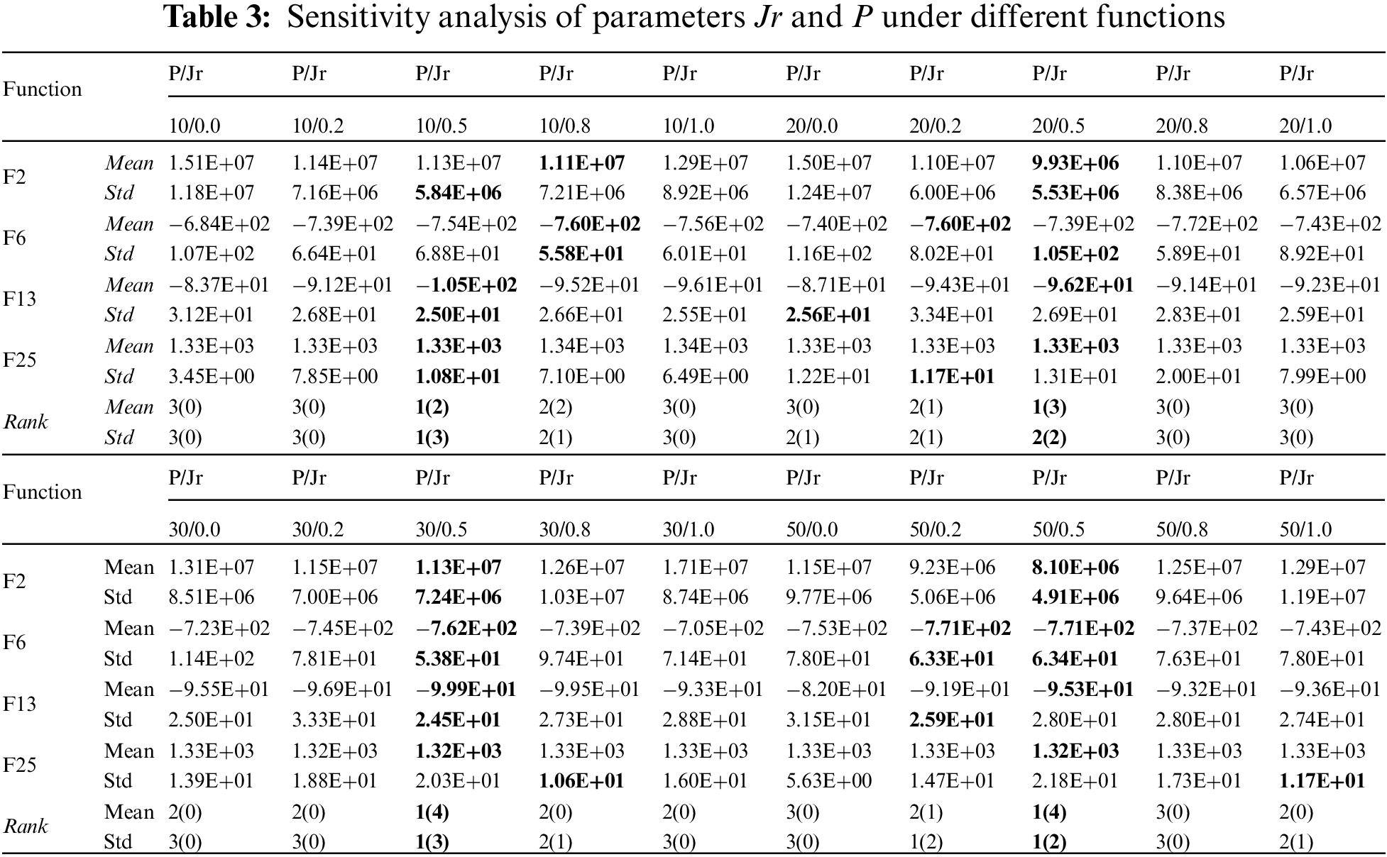
In the table, Mean signifies the average fitness values obtained from 30 independent runs of the algorithm, while Std denotes the standard deviation. Notably, the experiment data highlighted in bold font corresponds to the optimal results achieved. Additionally, the Rank column assigns rankings to the seven comparative algorithms. These rankings are determined by sorting the algorithm’s performance across various test functions. The numbers in parentheses indicate how many times the algorithm achieved the best result on such test functions. Based on these counts, the numbers outside the parentheses determine the final rankings of the seven algorithms. Ranking first also implies that the algorithm achieved the best results on more functions. From Table 3, it can be observed that different settings of Jr affect the algorithm’s performance on the test functions, leading to the following conclusions.

Conclusion 1: With a fixed population size P, as Jr increases from 0.0 to 1.0, the algorithm’s performance exhibits an initial improvement followed by a decline. This is evident when P = 10, Jr = 0.8 yields the best results for F2, while Jr = 0.5 is optimal for F6, F13, and F25. For P = 20/30/50, Jr = 0.5 ranks first in both the mean and standard deviation of final convergence accuracy across all four functions. This highlights the effectiveness of augmenting the probability of using the elite opposition-based search operator to improve the optimization accuracy of WOA. However, the algorithm is limited by the maximum number of fitness function calls during the search. As Jr increases, the number of fitness function calls per iteration also increases, which reduces the overall number of iterations. This, in turn, leads to a decrease in optimization accuracy. Therefore, Jr = 0.5 is the most appropriate value.

Conclusion 2: With Jr fixed, as P increases from 10 to 50, the algorithm’s performance shows a consistent improvement trend. Taking Jr = 0.5 as an example, for F2 and F6, the best results are obtained when P = 50. For F13, P = 30 performs the best, and for F25, P = 30 and 50 exhibits the best performance. This conclusion differs somewhat from Conclusion 1, mainly due to the simplicity of unimodal functions, where increasing P can fully exploit the benefits of chaotic initialization and opposition-based initialization operators, effectively improving the algorithm’s optimization accuracy. However, multimodal and composite functions are relatively complex, making them more challenging to optimize. As P increases, the algorithm is also constrained by the maximum fitness function calls during the search, leading to a decrease in optimization efficiency. Therefore, P = 30 is the most suitable value.

3.3 Experiment 2: Comparison of Olchwoa with Other Metaheuristic Algorithms

3.3.1 Performance Comparison for CEC 2013

To illustrate the merits of the proposed OLCHWOA algorithm, this section conducts comparative analyses involving several optimization algorithms, including PSO, HHO, AVOA, WOA, OLWOA, CHWOA, and OLCHWOA. The selection of these algorithms is grounded in three primary considerations. Firstly, PSO, introduced in 1995, is a well-established heuristic algorithm known for its enduring competitiveness. Secondly, both HHO and AVOA are distinguished by their simplicity in principles, minimal parameter requirements, and robust global search capabilities, rendering them highly competitive and advanced optimization algorithms that have emerged in recent years. Lastly, WOA serves as the foundational basis for OLCHWOA. Subsequently, OLWOA and CHWOA, arising from the incorporation of opposition-based learning and chaos mechanisms into WOA, respectively, naturally establish a basis for comparison with OLCHWOA, which integrates both enhancement operators. The effectiveness of each operator within OLCHWOA will be validated through ablation experiments. Following the discussion presented in Section 3.3.1, the algorithm has established the optimal parameter values for Jr and P. The parameter configurations for OLCHWOA and the other six comparative algorithms are provided in Table 4.

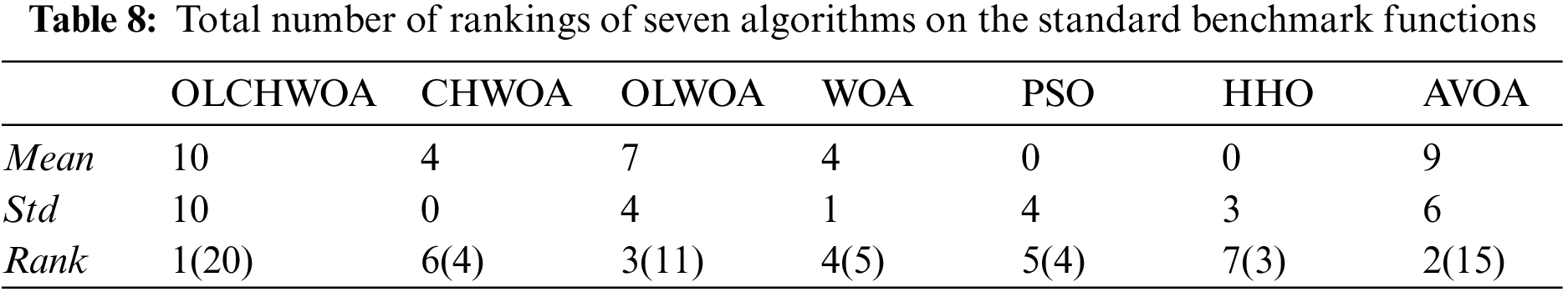
In this experiment, the Max_Fitness was set to 10,000. The experimental results for the seven compared algorithms on unimodal, multimodal, and composite functions are presented in Tables 5 to 7. Additionally, Table 8 summarizes the rankings of the seven algorithms. The following conclusions can be clearly drawn from the results presented in Tables 5–8.

Conclusion 1: On unimodal functions, the OLCHWOA algorithm distinctly excels. This is supported by OLCHWOA achieving the highest rank on four test functions (F1, F2, F4, and F5) in terms of mean values, as well as one test function (F1) in terms of standard deviation. These results underscore OLCHWOA’s capacity to achieve optimal performance across a significant range of unimodal functions.

Conclusion 2: On multimodal functions, both the OLCHWOA and AVOA algorithms exhibit the best performance in terms of algorithm convergence accuracy, with a relatively greater advantage over other algorithms. In terms of algorithm stability, OLCHWOA surpasses AVOA, as evidenced by OLCHWOA obtaining the first rank in mean and standard deviation values for five test functions, while AVOA only secures the first rank in these categories for five and three functions, respectively.

Conclusion 3: Regarding composite functions, the OLCHWOA algorithm ranks second in mean values and first in standard deviation. This is prominently observed in OLCHWOA, ranking first in mean values for one test function (F24), second for three test functions (F21, F25, F26), and first in standard deviation for four test functions (F21, F25, F26, F28). These outcomes confirm the algorithm’s ability to produce commendable results when faced with the most complex benchmark problems.

Conclusion 4: Among the three types of functions, the OLCHWOA algorithm demonstrates the highest performance, followed by the AVOA and OLWOA algorithms. This is primarily evident in OLCHWOA ranking first in mean values for all 28 test functions and first in standard deviation for 10 of them, placing it in a leading position, as detailed in Table 8. Additionally, Table 8 underscores that OLWOA obtains an overall superior ranking when compared to CHWOA, signifying that the opposition-based search operator exerts a more significant influence than the chaotic initialization operator in enhancing the standard WOA algorithm. This observation implies that OLCHWOA achieves a well-balanced outcome and exhibits a heightened potential for approaching the theoretical optimal solutions of these test functions. This is largely attributed to the contributions of the opposition-based search operator.

3.3.2 Comparison of Olchwoa and Other Algorithms under Different P Values

The sensitivity analysis in Section 3.2 discusses the impact of the population size P only on the OLCHWOA algorithm. To verify whether the algorithm proposed can still maintain its relative advantage as the P increases compared to other algorithms, this section selects eight representative test functions from CEC2013 for a comprehensive examination. Specifically, considering the scenarios of P = 50 and P = 100, maintaining all other parameters identical to those outlined in Section 3.3.1. The results of these experiments are outlined in Tables 9 and 10. After conducting a meticulous analysis, the following conclusions have been drawn:

Conclusion 1: When P = 50, OLCHWOA outperforms the other six algorithms. This superiority is underscored by OLCHWOA achieving values that closely approach the global optimum on seven functions (F4, F7, F9, F13, F19, F24, and F26). The comprehensive ranking, based on both the mean and standard deviation, secures the top position.

Conclusion 2: When P = 100, OLCHWOA maintains a remarkable performance by attaining optimal values in five functions (F4, F7, F9, F24, and F26), with its comprehensive ranking, based on mean and standard deviation being first and second, respectively.

Conclusion 3: Combining the results from Section 3.3.1 when P = 30, it can be observed that as the population size increases, OLCHWOA’s solution accuracy hardly decreases. Notably, its performance remains consistently competitive relative to the other comparative algorithms. OLCHWOA demonstrates efficient global search capabilities, and its effectiveness remains unhindered with the augmentation of the population size.

3.3.3 Convergence Analysis

To illustrate how the improved strategy impacts algorithm convergence speed more intuitively, Fig. 3 compares the average convergence curves of seven algorithms in different test functions. In view of space constraints within this paper, this section focuses on eight representative test functions. Specifically, F1 and F5 represent the convergence curves for unimodal functions. F6, F13, F15, and F20 illustrate the convergence curves for multimodal functions, while F24 and F26 depict the convergence curves for composite functions. The algorithm parameter settings align with those established in Section 3.3.1. The insights gleaned from Fig. 3 are as follows:

Figure 3: Convergence graphs of eight functions

Conclusion 1: From the perspective of solution accuracy, as the number of fitness calls increases, OLCHWOA consistently gravitates towards the global optimum and ultimately attains higher convergence accuracy in comparison to the other six comparative algorithms across F1, F5, F6, F13, F20, and F24. This observation underscores the robust ability of the OLCHWOA to effectively escape local optima across the three categories of test functions. Concurrently, the OLWOA algorithm, similar to OLCHWOA, also demonstrates commendable convergence accuracy. This parallel suggests that the incorporation of opposition-based learning greatly enhances the global search capability of WOA.

Conclusion 2: From the perspective of the initial population’s quality, OLCHWOA exhibits lower initial fitness values in the average convergence curves for the eight test functions, surpassing the original WOA and CHWOA. This suggests that the introduced chaotic initialization operator and opposition-based initialization operator in this paper effectively improve the quality of the initial population.

Conclusion 3: From the perspective of convergence speed, OLCHWOA exhibits slower convergence speed, which is particularly evident in complex functions such as F13, F15, and F20. Additionally, CHWOA demonstrates the fastest convergence on functions F1, F6, F13, and F15, while OLWOA exhibits the fastest convergence on function F5. AVOA showcases the most rapid convergence on functions F20 and F26, while OLCHWOA converges most swiftly on function F24. This observation suggests that the introduction of the chaotic initialization operator and opposition-based initialization operator, as detailed in this paper, has the potential to enhance convergence speed, especially on simpler test functions. However, their effectiveness is limited when faced with more complex problem sets. Per the “no free lunch theorem” [74], improving an algorithm’s performance in terms of both convergence speed and solution accuracy simultaneously presents a significant challenge. The proposed OLCHWOA algorithm significantly improves solution accuracy while sacrificing some convergence speed, which is one of the limitations of this algorithm.

3.3.4 Wilcoxon Rank Sum Test

This paper compares the seven algorithms using the Mean and Std in Section 3.3. However, the results of only 30 independent runs cannot convincingly support the superiority of the OLCHWOA algorithm since there is still a certain probability that the algorithm performs better by chance. For this reason, this section applies the Wilcoxon rank sum test to measure the significance of the differences between different algorithms at the statistical level [75]. The study takes into account the results obtained by seven algorithms independently solving 28 test functions for 30 independent runs as samples and tests them under the condition of a confidence level of 0.05 to determine if there were any significant differences between the results obtained by OLCHWOA and the other six algorithms. A significance threshold of p < 0.05 was applied. If the p-value exceeds this threshold, the optimization outcomes of the two algorithms are considered indistinguishable. Table 11 presents the results of the Wilcoxon rank-sum test. Results with p-values greater than 0.1 are shown in bold.

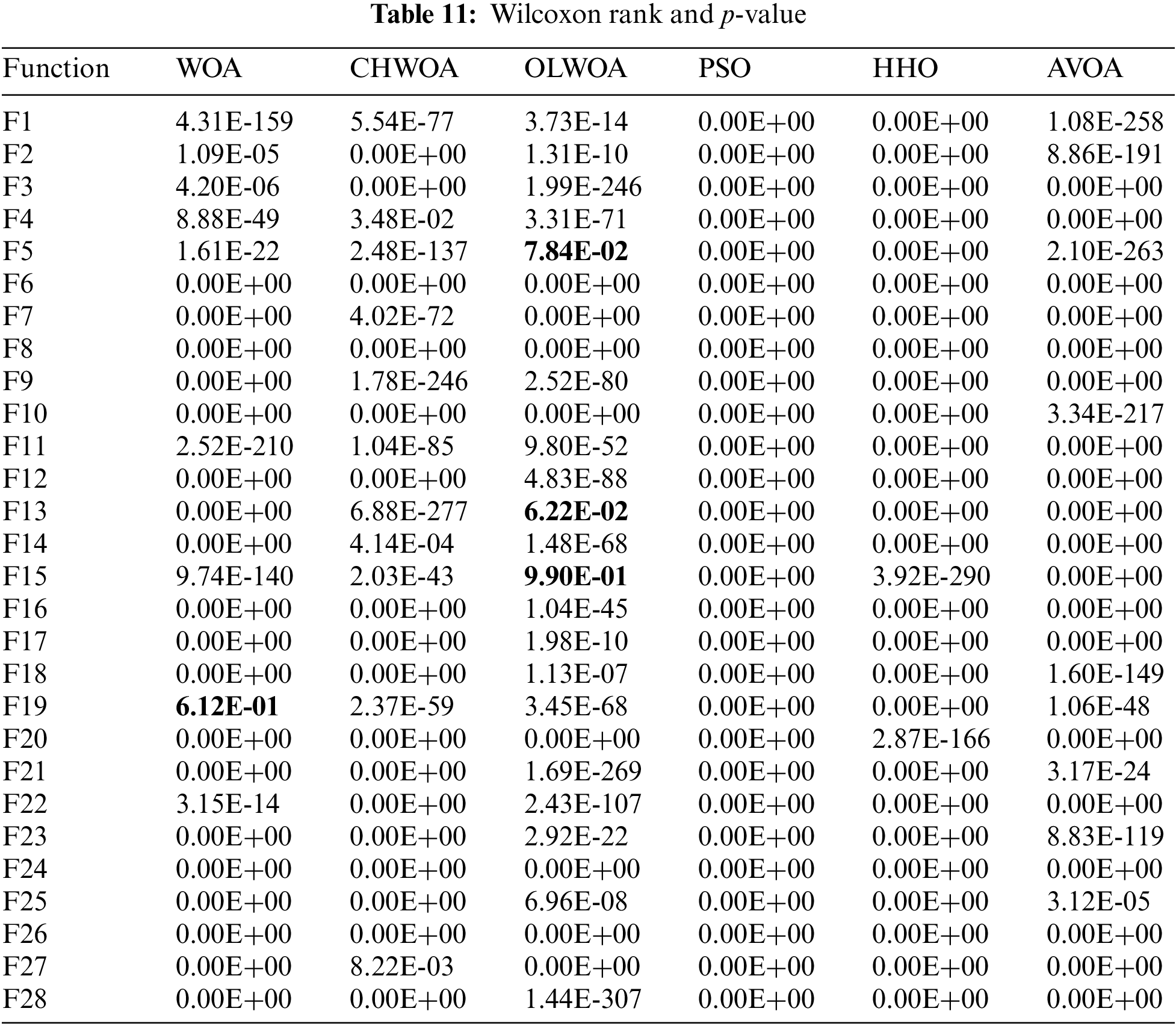
As indicated in Table 11, both OLCHWOA and OLWOA exhibit p-values exceeding 5% for F5, F13, and F15, while OLCHWOA and WOA attain p-values exceeding 5% for F19. Nevertheless, for the remaining test functions, all obtained p-values are below 0.05. This statistical analysis underscores that OLCHWOA differs significantly from and outperforms the compared algorithms in these instances. Using the experiments presented in Sections 3.3.1, 3.3.3, and 3.3.4, it is concluded that the OLCHWOA combined with chaos mechanism and opposition-based learning strategy has higher convergence accuracy, improved ability to jump out of local optimal solutions and better stability than six other optimization algorithms.

3.4 Experiment 3: Comparisons between Olchwoa and Other Whale Variants

To provide a comprehensive evaluation of the merits and drawbacks of OLCHWOA, it was compared with four recent WOA variants, including ACWOA [76], RDWOA [77], TBWOA [78], and MEWOA [79]. These algorithms have been published in reputable journals and are widely recognized as benchmarks. Table 12 presents the average convergence accuracy and stability for 10 CEC2019 functions. The experimental results for these four WOA variants are sourced from reference [80], while the experiments for OLCHWOA are based on our simulation results. To ensure a fair comparison, this paper replicated the experimental conditions mentioned in the reference (Max_fitness = 15000).

As shown in the table, OLCHWOA, MEWOA, and ACWOA consistently achieved the highest average rankings in terms of mean convergence accuracy. OLCHWOA obtained five first-place rankings, MEWOA obtained four first-place rankings, and ACWOA obtained one first-place ranking. Similarly, when considering standard deviation, these algorithms also emerged as frontrunners, with 5, 2, and 1 instances ranking first, respectively. The OLCHWOA algorithm consistently obtained the highest average ranking, indicating its superior global search capability compared to the other four recent WOA variants, especially when it comes to solving complex optimization problems.

3.5 Experiment 4: Application of Engineering Problems

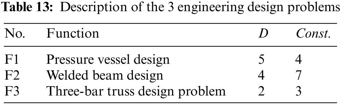
Given the intricacies presented by constraints in real-world optimization challenges, traditional algorithms often struggle to find solutions. This section evaluates OLCHWOA’s performance in three specific scenarios: the pressure vessel design problem, the three-bar truss design problem, and the welded beam design problem. Table 13 succinctly outlines the dimensions and the number of constraints. For more detailed information, please refer to references [79,80].

3.5.1 Pressure Vessel Design Problem

The objective of the pressure vessel design problem is to find the design solution with the minimum cost. Here, x1, x2, x3, x4, and f(x) represent the shell thickness, head thickness, vessel internal radius, cylindrical section length, and minimum cost, respectively. To evaluate OLCHWOA’s optimization results in the pressure vessel design problem, a comparison was made with ten algorithms selected from reference [79]. OLCHWOA’s simulation results were obtained from our experiments, and the algorithm parameters were set consistent with Section 3.3.1. The maximum fitness function calls for the experiments was set to 15,000, following the conditions outlined in the reference. The experimental results in Table 14 show that OLCHWOA outperformed other algorithms, achieving the best optimization results.

3.5.2 Three-Bar Truss Design Problem

The objective of this problem is to minimize the volume of its members while satisfying stress constraints for the bars. This endeavor entailed a meticulous comparison that involved the careful selection of 7 algorithms from reference [79]. Here, x1, x2, and f(x) represent the cross-sectional areas of the two bars and the minimum volume, respectively. Similar to Section 3.5.1, the simulation results of OLCHWOA were obtained from our experiments. The experimental results in Table 15 show that algorithms such as DEPSO, WOAmM, MEWOA, and OLCHWOA obtain approximate optimal solutions. This suggests that these algorithms faced challenges despite having only three constraint conditions.

3.5.3 Welded Beam Design Problem

The objective of optimizing this problem is to minimize the cost. Here, x1, x2, x3, x4, and f(x) respectively represent the length of the steel connecting rod, the thickness of the weld, the height of the steel rod, the thickness of the steel rod, and the minimum cost. The optimization results obtained by OLCHWOA in the welded beam design problem proposed in this paper were compared with those of eight algorithms from reference [80]. The results are presented in Table 16. It was observed that e-mPSOBSA and CLPSO achieved the best results, while the OLCHWOA ranked third, providing solutions that are highly competitive among the eight algorithms.

4  Application of Olchwoa Algorithm in RV Forecasting

4.1 Lstm Model

In this paper, the LSTM model serves as the benchmark model for RV prediction. LSTM utilizes memory units to store information and gate structures to discard unnecessary information, resulting in an extended memory. Unlike traditional neural networks, LSTM is composed of memory blocks. Fig. 4 shows the detailed structure of a memory block, which consists of a memory unit ct, input gate it, forgetting gate gt, and an output gate ot. According to Eqs. (19)–(24), the three gates it, gt , ot and the memory unit ct can be calculated, where xt represents the input at time t, ht represents the hidden state, U and W denote the weight matrix, b denotes the bias term, σ(⋅) is a sigmoid function.

gt=σ(Ugxt+Wght−1+bf)(19)

it=σ(Uixt+Wiht−1+bi)(20)

c~t=tan⁡h(Ucxt+Wcht−1+bc)(21)

ct=gt∗ct−1+it∗c~t(22)

ot=σ(Uoxt+Woht−1+bo)(23)

ht=ot∗tan⁡h(ct)1(24)

Figure 4: Structure of LSTM

4.2 Rv Prediction Model Based on OLCHWO-LTSM

The OLCHWO-LTSM model is designed to evaluate the effectiveness of the OLCHWOA in optimizing the LSTM-based RV prediction model. Fig. 5 depicts the execution flow diagram for the RV prediction model based on OLCHWO-LTSM. The diagram includes the following modules: Data Processing Module, Model Training Module, Parameter Optimization Module, and Evaluation Module.

Figure 5: RV prediction framework based on OLCHWOA-LSTM

Data Processing Module: Firstly, the dataset is split into a training and a testing set. The first 90% of the data is used to train the LSTM model, while the remaining 10% is used to test and validate the algorithm’s predictive performance. Prior to inputting variables, data normalization is performed.

Model Training Module:To enhance the model’s ability to make nonlinear predictions, the LSTM architecture utilizes a three-layer structure. This configuration includes a single LSTM hidden layer along with two fully connected layers, as visually represented in Fig. 5.

Parameter Optimization Module: Within this module, the OLCHWOA algorithm is strategically utilized to coordinate the optimization of four crucial hyperparameters inherent to the LSTM model. These parameters include the number of nodes within the LSTM layer (ls1), the number of nodes in the fully connected layer (ls2), the dropout parameter of the LSTM (dp), and the proportion of the validation set (vs). In essence, this optimization endeavor aims to identify the optimal parameter configuration, thereby improving the predictive capacity of the LSTM model. The parameter search intervals specified for these hyperparameters of interest are as follows: ls1∈ [1, 200], ls2∈ [1, 200], dp ∈ [0.01, 0.9], and vs.∈ [0.01, 1]. It is worth noting that the remaining parameters governing the operation of the LSTM model adhere to a uniform standardization. This involves setting a fixed batch size of 512, running 50 iterations, using the Adam optimizer, and employing the Mean Squared Error (MSE) as the loss function.

Evaluation Module diligently deploys the fine-tuned LSTM model to facilitate the prediction of RV values.

4.3 Experimental Settings

4.3.1 Data

The China Securities Index 300 (CSI 300) futures were introduced on April 16, 2010, and have since become the most actively traded stock index futures product in the Chinese market. This article focuses on high-frequency data of the CSI 300 Index, covering the period from January 04, 2010, to March 20, 2020, which comprises a total of 2,480 trading days. The specific calculation of RV data is based on Anderson et al. [81]. The process is shown below.

Using a sampling frequency of 5 min per trading day and obtaining the opening and closing prices every 5 min, 48 high-frequency returns can be obtained for a single trading day. In total, there would be 119,040 high-frequency returns. Price series are expressed as Pt,d, t = 1,2,3,… ,2480, d = 0,1,2,3,…, 48, where Pt,0 represents the opening price at 9:30 on trading day t, and Pt,d represents the closing price at the d-th 5-minute mark. Rt indicates the daily return, which is calculated using the closing prices of the two adjacent trading days. Here is the formula.

Rt=100(ln Pt,48–ln Pt−1,48)(25)

where t = 1,2,3,…,2480. Likewise, the high frequency return Rt,d for the 5-min period d-th on day t is calculated as indicated by the following formula:

Rt,d=100(ln Pt,d–ln Pt−1,d)(26)

where t = 1,2,3,…,2480, and d = 0,1,2,3,…,48.

The RV on day t can be estimated by the following formula:

RVt=∑d=1nt⁡Rt,d2(27)

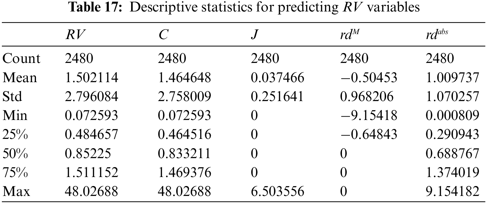
Jumpiness is a concept that pertains to the substantial shifts in volatility observed when significant information emerges within financial markets, often resulting in pronounced jumps. Drawing upon this notion of jumpiness, this study introduces continuous volatility denoted as C and jump volatility denoted as J as inputs into the LSTM model. Additionally, volatility exhibits asymmetric characteristics, indicating that positive and negative news in the market have varying effects on volatility. Negative news tends to increase volatility. Based on this perspective, two predictive variables are introduced: the absolute value of volatility on down days, denoted as rdM, and the absolute value of daily volatility, denoted as rdabs.

To evaluate the performance of the OLCHWOA-LSTM model in predicting RV for the CSI 300 Index, the previous period’s realized volatility (RV), continuous volatility (C), jump volatility (J), the absolute value of the down day’s volatility (rdM,), and the absolute value of the daily volatility (rdabs) are used as inputs. The model is designed to forecast RV for the next trading day based on a time series of five variables spanning the past 22 trading days. The data is sourced from the RESET HF Database, and Table 17 provides descriptive statistics for each indicator.

4.3.2 Evaluation Metrics

For the purpose of better reflecting the predicted value error, this paper uses four commonly used evaluation metrics, namely Mean Absolute Error (MAE), Mean Square Error (MSE), Heteroscedasticity adjusted MAE (HMAE), and Heteroscedasticity adjusted MSE (HMSE). The formulas for calculating the four evaluation indicators are as follows:

MAE=1T∑|V^t−RVt|(28)

MSE=1T∑(V^t−RVt)2(29)

HMAE=1T∑|1−V^t/RVt|(30)

HMSE=1T∑(1−V^t/RVt)2(31)

where V^t is the predicted value of RV at moment t, RVt is the true value, and T is the number of samples.

4.4 Environment, Comparison Models and Their Parameter Settings

In this section, the TensorFlow2.2 version is used to build the deep learning framework of LSTM, and the rest of the computer configuration is the same as in Section 3. ARFIMA and HAR are used as comparison models in this paper. The following is a brief introduction to their principles.

HAR is based on the heterogeneous market hypothesis. In order to present volatility generated by different traders, the HAR model uses daily RV, weekly RV, and monthly RV to show volatility generated by short-term, medium-term, and long-term traders, respectively. The model uses 1-day, 5-days, and 22-days as the trading time scales for each of the three investors. This model is described by the following formula:

RVt+1=β0+βDRV1+βWRV5+βMRV22(32)

where RV1, RV5, and RV22 denote daily RV, weekly RV, and monthly RV, respectively.

The ARFIMA model takes into account both long-term and short-term memory of time series. The specific formula is as follows:

φp(L)(1−L)d(Xt−μ)=θq(L)at(33)

where μ is the series mean, |d| < 0.5, (1-L)d is the fractional difference factor, order p and q are short memory factors, and order d indicates long-term memory.

The HAR and ARFIMA models are the most classic RV prediction models and are considered reasonable as comparative models. They are implemented using the HARModel package and forecast package in the R language. LSTM is the basic model for RV prediction. To evaluate the performance of OLCHWOA in RV prediction, the PSO-LSTM model, HHO-LSTM model, WOA-LSTM model, OLWOA-LSTM model, CHWOA-LSTM model, and OLCHWOA-LSTM model were compared.

Table 18 lists the parameter settings of the above 9 models, which are set according to the results of the training set experiments. The HAR model contains four parameters: beta0, beta1, beta5, and beta22, which represent the average level of volatility and the impact of three different frequencies of market participants on RV, daily, weekly, and monthly, respectively. The results of parameter estimation show that all four coefficients are significant at the 1% confidence level. The ARFIMA model contains eight parameters. The difference term d is a score between −0.5 and 0.5, which is used to capture long-term memory and can be obtained by calculating the Hurst exponent, and its formula is d = Hurst-0.5. AR1 to AR5 are the autocorrelation coefficients of the model, while MA1 and MA2 are the moving average coefficients, and these eight parameters are determined by the AIC criterion. LSTM model parameters ls1, ls2, dp, and vs have the same meanings as those in Section 4.2. Additionally, P and Max_Fitness have the same meanings as those described in Section 3.2. There are several types of LSTM models that are based on three-layer network structures, but their optimal parameters vary.

4.5 Experimental Results

Table 19 shows the experimental results of the nine comparison models mentioned in Section 4.4 on the RV dataset. According to Table 19, the following conclusions can be drawn:

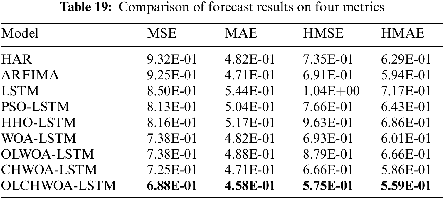
Conclusion 1: The OLCHWOA-LSTM model has the best performance. This is demonstrated by the fact that the OLCHWOA-LSTM model outperforms the HAR model, ARFIMA model, LSTM model, PSO-LSTM model, HHO-LSTM model, WOA-LSTM model, OLWOA-LSTM model, and CHWOA-LSTM model in indicator MSE by 26.19%, 25.58%, 19.05%, 15.31%, 15.71%, 6.76%, 6.73%, and 5.11%, respectively. MAE, HMSE, and HMAE also exhibit varying degrees of improvement. Consequently, the improved algorithm has advantages not only on standard test functions, but also in practical application problems.

Conclusion 2: Models optimized for LSTM parameters based on heuristic algorithms generally outperform classical models such as HAR and ARFIMA. It appears that the four metrics of OLWOA-LSTM, CHWOA-LSTM, and OLCHWOA-LSTM all outperform HAR and ARFIMA.

Conclusion 3: ARFIMA and HAR perform better than standard LSTMs. It is evident from this example that LSTM models require parameter optimization. It is impossible to exploit LSTM’s nonlinear prediction capabilities without optimization. This further demonstrates the necessity of conducting this study.

4.6 Discussion

The OLCHWOA-LSTM model presented is an interesting study that deepens understanding of how LSTM technology contributes to research on RV. Research in the past has focused on optimizing LSTM hyperparameters using an exhaustive method [82–84], which had the shortcomings of being time-consuming and yielding poor results. This limitation has just been addressed in this study. Moreover, the OLCHWOA-LSTM model is highly competitive in predicting RV problems. There are two main reasons for this.

First, the OLCHWOA-LSTM model can capture the nonlinear characteristics of RV and, therefore, statistically significantly outperforms HAR and ARFIMA, which are currently the most commonly used models in the industry. For RV prediction, ARFIMA can capture long-term memory and aggregation characteristics, while HAR can capture both aggregation and market heterogeneity characteristics. Compared to HAR and ARFIMA, the OLCHWOA-LSTM model can effectively capture the long memory and aggregation characteristics of RV by leveraging the inherent capabilities of LSTM. Furthermore, it can also account for the heterogeneity and asymmetry of RV through its input variables. Additionally, the LSTM model is capable of capturing nonlinearity in the time series of RV. The OLCHWOA-LSTM model not only exhibits the characteristics of ARFIMA and HAR models, but it also offers the advantages of nonlinear feature acquisition and asymmetric capture, making it statistically significant.

Second, the OLCHWOA-LSTM model is statistically significantly superior to other machine learning models as a result of its hyperparameter optimization. RV prediction is essentially a time series prediction problem, and the LSTM model is specifically designed to handle it. By automating the hyperparameter optimization process, OLCHWOA further enhances the benefits of LSTM when dealing with time series data.

5  Conclusions and Future Works

This paper proposes a streamlined and efficient enhancement to the Whale Optimization Algorithm (WOA), called OLCHWOA in this manuscript. This improvement incorporates several new operators, including a chaotic initialization operator based on logistic sequences, an opposition-based initialization operator, and an elite opposition-based learning operator based on the parameter Jr. These operators are introduced into the original WOA algorithm. The proposed algorithm offers several advantages: (1) The chaotic initialization and opposition-based initialization operators enhance the diversity of the OLCHWOA population in the early stages, endowing the algorithm with strong exploration capabilities and contributing to improved search efficiency. (2) The opposition-based search operator enables the algorithm to maintain robust local exploitation capabilities even in the later iterations, allowing it to attain superior solution accuracy in optimization tasks and a greater probability of finding the global optima of complex functions. (3) OLCHWOA is straightforward to implement and delivers satisfactory performance. The introduced enhancement strategies improve the algorithm’s search efficiency without compromising its time complexity. (4) Extensive experiments and diverse application scenarios validate the reliability of the OLCHWOA algorithm. Four sets of experiments were conducted to investigate the performance of OLCHWOA in solving complex optimization problems. The results indicated that Jr = 0.5/P = 30 represents the most competitive parameter setting. Firstly, the impact of different combinations of parameters, including the jump rate Jr and the population size P, on the performance of OLCHWOA are discussed. Secondly, the proposed OLCHWOA algorithm is evaluated on 28 CEC2013 standard test functions and 10 CEC2019 standard test functions. It was compared with various types of heuristic algorithms, including traditional PSO, WOA, recently proposed HHO and AVOA, partially improved algorithms of WOA like OLWOA, CHWOA, and variants of WOA algorithms such as ACWOA. Simulation results demonstrated that OLCHWOA outperformed the other compared algorithms significantly in terms of convergence accuracy and stability. Furthermore, to assess the algorithm’s capability to solve real-world complex optimization problems, OLCHWOA was experimented with three constrained engineering design problems. The results indicated that the proposed algorithm also exhibited superiority and applicability. Lastly, OLCHWOA was used to perform hyperparameter auto-tuning for the LSTM model and applied to the RV prediction problem. Experimental results based on the CSI 300 dataset demonstrated that the OLCHWOA-LSTM model achieved the highest accuracy and robustness in RV prediction. This illustrates the high competitiveness and efficient search capability of our algorithm in solving practical problems under similar conditions.

Nevertheless, OLCHWOA still exhibits certain limitations. Firstly, although the proposed algorithm exhibits a high global search capability, it does not consistently achieve top performance across all functions in CEC2013 and CEC2019. It struggles to converge to the optimum in certain high-dimensional functions. Furthermore, the use of the opposition-based learning strategy in OLCHWOA enables it to maintain strong exploitation capabilities in subsequent iterations. Nevertheless, this strategic inclusion increases the frequency of fitness function invocation per iteration, which slows down convergence, especially when dealing with complex composite functions.

In future investigations, our team will focus on three specific domains to further enhance the performance of OLCHWOA: (1) The jump rate Jr in this paper was set as a fixed value, but it may not necessarily be the optimal choice. Therefore, the adaptive adjustment mechanism of parameter Jr will be considered. (2) OLCHWOA exhibits a slower convergence rate, and research on enhancing its convergence speed will be prioritized. (3) While OLCHWOA has demonstrated success in continuous function optimization, additional validation is required to evaluate its effectiveness in addressing discrete optimization challenges.

Acknowledgement: The authors thank the anonymous reviewers and editors for their valuable comments and suggestions.

Funding Statement: The National Natural Science Foundation of China (Grant No. 81973791) funded this research.

Author Contributions: The authors confirm contribution to the paper as follows: study conception and design: Xiang Wang, Yibin Guo; data collection: Liangsa Wang, Han Li; analysis and interpretation of results: Xiang Wang, Liangsa Wang, Han Li; draft manuscript preparation: Liangsa Wang, Han Li. All authors reviewed the results and approved the final version of the manuscript.

Availability of Data and Materials: Researchers can obtain the data supporting the findings of this study by contacting the corresponding authors.

Conflicts of Interest: The authors declare that they have no conflicts of interest to report regarding the present study.

References

1. T. Bollersleva and H. O. Mikkelsen, “Modeling and pricing long memory in stock market volatility,” Journal of Econometrics, vol. 73, no. 1, pp. 151–184, 1996. [Google Scholar]

2. F. X. Diebold and G. D. Rudebusch, “Long memory and persistence in aggregate output,” Journal of Monetary Economics, vol. 24, no. 2, pp. 189–209, 1989. [Google Scholar]

3. Y. Ding, D. Kambouroudis and D. G. McMillan, “Forecasting realised volatility: Does the LASSO approach outperform HAR?,”Journal of International Financial Markets, Institutions and Money, vol. 74, pp. 101386, 2021. [Google Scholar]

4. T. G. Andersen, T. Bollerslev, F. X. Diebold and P. Labys, “The distribution of realized exchange rate volatility,” Journal of the American Statistical Association, vol. 96, no. 453, pp. 42–55, 2001. [Google Scholar]

5. P. Giot and L. Sébastien, “Modelling daily value-at-risk using realized volatility and aRCH type models,” Journal of Empirical Finance, vol. 11, no. 3, pp. 379–398, 2004. [Google Scholar]

6. S. Degiannakis, “ARFIMAX and ARFIMAX-TARCH realized volatility modeling,” Journal of Applied Statistics, vol. 35, no. 10, pp. 1169–1180, 2008. [Google Scholar]

7. W. Zhou, J. Pan and X. Wu, “Forecasting the realized volatility of CSI 300,” Physica A: Statistical Mechanics and its Applications, vol. 531, pp. 121799, 2019. [Google Scholar]

8. M. Izzeldin, M. K. Hassan, V. Pappas and M. Tsionas, “Forecasting realised volatility using ARFIMA and HAR models,” Quantitative Finance, vol. 19, no. 10, pp. 1627–1638, 2019. [Google Scholar]

9. O. E. Barndorff-Nielsen and N. Shephard, “Power and bipower variation with stochastic volatility and jumps,” Journal of Financial Economics, vol. 2, no. 1, pp. 1–37, 2004. [Google Scholar]

10. T. G., Andersen, T. Bollerslev and F. X. Diebold, “Roughing it up: Including jump components in the measurement, modeling, and forecasting of return volatility,” Review of Economics & Statistics, vol. 89, no. 4, pp. 701–720, 2007. [Google Scholar]

11. T. Bollerslev, A. J. Patton and R. Quaedvlieg, “Exploiting the errors: A simple approach for improved volatility forecasting,” Journal of Econometrics, vol. 192, no. 1, pp. 1–18, 2016. [Google Scholar]

12. S. Hochreiter and J. Schmidhuber, “Long short-term memory,” Neural Computation, vol. 9, no. 8, pp. 1735–1780, 1997. [Google Scholar] [PubMed]

13. N. Maknickienė and A. Maknickas, “Application of neural network for forecasting of exchange rates and forex trading,” in the 7th Int. Scientific Conf. “Business and Management”, Vilnius, Lithuania, pp. 122–127, 2012. [Google Scholar]

14. K. Chen, Y. Zhou and F. Dai, “A LSTM-based method for stock returns prediction: A case study of China stock market,” in IEEE Int. Conf. on Big Data (Big Data), Santa Clara, CA, USA, pp. 2823–2824, 2015. [Google Scholar]

15. H. Y. Kim and C. H. Won, “Forecasting the volatility of stock price index: A hybrid model integrating lSTM with multiple gARCH-type models,” Expert Systems with Applications, vol. 103, pp. 25–37, 2018. [Google Scholar]

16. Y. Hu, J. Ni and L. Wen, “A hybrid deep learning approach by integrating LSTM-ANN networks with GARCH model for copper price volatility prediction,” Physica A: Statistical Mechanics and its Applications, vol. 557, pp. 124907, 2020. [Google Scholar]

17. Y. Lin, Z. Lin, Y. Liao, Y. Li J. Xu et al., “Forecasting the realized volatility of stock price index: A hybrid model integrating CEEMDAN and LSTM,” Expert Systems with Applications, pp. 117736, 2022. [Google Scholar]

18. X. Chen and Y. Hu, “Volatility forecasts of stock index futures in China and the US–a hybrid lSTM approach,” PLoS One, vol. 17, no. 7, pp. e271595, 2022. [Google Scholar]

19. J. H. Holland, “An overview,” in Adaptation in Natural and Artificial Systems: An Introductory Analysis with Applications to Biology, Control, and Artificial Intelligence, MIT Press, pp. 159–170, 1992. [Google Scholar]

20. S. Kirkpatrick, C. D. Gelatt and A. Vecchi, “Optimization by simulated annealing,” Science, vol. 220, pp. 671–680, 1983. [Google Scholar] [PubMed]

21. F. Glover, “Future paths for integer programming and links to artificial intelligence,” Computers & Operations Research, vol. 13, no. 5, pp. 533–549, 1986. [Google Scholar]

22. M. Dorigo, “Optimization, learning and natural algorithms,” Ph.D. dissertation, Politecnico di Milano, Italian, 1992. [Google Scholar]

23. G. Venter and J. Sobieszczanski-Sobieski, “Particle swarm optimization,” AIAA Journal, vol. 41, no. 8, pp. 129–132, 2003. [Google Scholar]

24. R. Storn and K. Price, “DE–a simple and efficient heuristic for global optimization over continuous space,” Journal of Global Optimization, vol. 114, no. 4, pp. 341–359, 1997. [Google Scholar]

25. G. G. Wang, X. Zhao and S. Deb, “A novel monarch butterfly optimization with greedy strategy and self-adaptive,” in 2015 Second Int. Conf. on Soft Computing and Machine Intelligence (ISCMI), Hong Kong, China, pp. 45–50, 2015. [Google Scholar]

26. R. Salgotra and U. Singh, “The naked mole-rat algorithm,” Neural Computing and Applications, vol. 31, no. 12, pp. 8837–8857, 2019. [Google Scholar]

27. A. A. Mohamed, Y. S. Mohamed, A. A. El-Gaafary and A. M. Hemeida, “Optimal power flow using moth swarm algorithm,” Electric Power Systems Research, vol. 142, pp. 190–206, 2017. [Google Scholar]

28. A. A. Heidari, S. Mirjalili, H. Faris, I. A. Mafarja and H. Chen, “Harris hawks optimization: Algorithm and applications,” Future Generation Computer Systems, vol. 97, pp. 849–872, 2019. [Google Scholar]

29. F. S. Gharehchopogh, A. Ucan, T. Ibrikci, B. Arasteh and G. Isik, “Slime mould algorithm: A comprehensive survey of its variants and applications,” Archives of Computational Methods in Engineering, vol. 30, no. 4, pp. 2683–2723, 2023. [Google Scholar] [PubMed]

30. F. S. Gharehchopogh and T. Ibrikci, “An improved african vultures optimization algorithm using different fitness functions for multi-level thresholding image segmentation,” Multimedia Tools and Applications, 2023. [Google Scholar]

31. K. M. Ong, P. Ong and C. K. Sia, “A carnivorous plant algorithm for solving global optimization problems,” Applied Soft Computing, vol. 98, pp. 106833, 2020. [Google Scholar]

32. Y. Yang, H. Chen, A. A. Heidari and A. H. Gandomi, “Hunger games search: Visions, conception, implementation, deep analysis, perspectives, and towards performance shifts,” Expert Systems with Applications, vol. 177, pp. 114864, 2021. [Google Scholar]

33. H. Mohammadzadeh and F. S. Gharehchopogh, “A multi-agent system based for solving high-dimensional optimization problems: A case study on email spam detection,” International Journal of Communication Systems, vol. 34, no. 3, pp. e4670, 2021. [Google Scholar]

34. S. T. Shishavan and F. S. Gharehchopogh, “An improved cuckoo search optimization algorithm with genetic algorithm for community detection in complex networks,” Multimedia Tools and Applications, vol. 81, no. 18, pp. 25205–25231, 2022. [Google Scholar]

35. F. S. Gharehchopogh, “An improved harris hawks optimization algorithm with multi-strategy for community detection in social network,” Journal of Bionic Engineering, vol. 20, no. 3, pp. 1175–1197, 2023. [Google Scholar]

36. S. M. Abedi Pahnehkolaei, A. Alfi and J. A. Tenreiro Machado, “Analytical stability analysis of the fractional-order particle swarm optimization algorithm,” Chaos, Solitons & Fractals, vol. 155, pp. 111658, 2022. [Google Scholar]

37. S. M. Abedi Pahnehkolaei, A. Alfi and J. A. T. Machado, “Convergence boundaries of complex-order particle swarm optimization algorithm with weak stagnation: Dynamical analysis,” Nonlinear Dynamics, vol. 106, no. 1, pp. 725–743, 2021. [Google Scholar]

38. H. Shokri-Ghaleh, A. Alfi, S. Ebadollahi, A. Mohammad Shahri and S. Ranjbaran, “Unequal limit cuckoo optimization algorithm applied for optimal design of nonlinear field calibration problem of a triaxial accelerometer,” Measurement, vol. 164, pp. 107963, 2020. [Google Scholar]

39. F. S. Gharehchopogh, “Quantum-inspired metaheuristic algorithms: Comprehensive survey and classification,” Artificial Intelligence Review, vol. 56, no. 6, pp. 5479–5543, 2023. [Google Scholar]

40. S. Mirjaliliab and A. Lewis, “The whale optimization algorithm,” Advances in Engineering Software, vol. 95, pp. 51–67, 2016. [Google Scholar]

41. D. Cui, “Application of whale optimization algorithm in reservoir optimal operation,” Advances in Science and Technology of Water Resources, vol. 37, no. 3, pp. 72–76, 2017. [Google Scholar]

42. Y. Xu, Y. Chunming and Y. Yuanyuan, “Solving job-shop scheduling problem by quantum whale optimization algorithm,” Application Research of Computers, vol. 36, no. 4, pp. 21–25, 2019. [Google Scholar]

43. C. Zhao, H. U. Hengxing, B. Chen, Y. Zhang and J. Xiao, “Bearing fault diagnosis based on the deep learning feature extraction and WOA SVM state recognition,” Journal of Vibration and Shock, vol. 38, no. 10, pp. 31–37, 2019. [Google Scholar]

44. P. Niu, Z. Wu, Y. Ma, C. Shi and J. Li, “Prediction of steam turbine heat consumption rate based on whale optimization algorithm,” vol. 68, no. 3, pp. 1049–1057, 2017. [Google Scholar]

45. X. U. Yufei, F. Qian, M. Yang, D. U. Wenli and W. Zhong, “Improved whale optimization algorithm and its application in optimization of residue hydrogenation parameters,” CIESC Journal, vol. 69, no. 3, pp. 891–899, 2018. [Google Scholar]

46. R. L. Haupt and S. E. Haupt, Practical Genetic Algorithms, New York, NY, USA: John Wiley & Sons, pp. 27–50, 2003. [Google Scholar]

47. G. Ning, D. Cao and M. de la Sen, “Improved whale optimization algorithm for solving constrained optimization problems,” Discrete Dynamics in Nature and Society, vol. 2021, pp. 8832251, 2021. [Google Scholar]

48. P. Gou, B. He, Z. Yu and P. I. Lazaridis, “A node location algorithm based on improved whale optimization in wireless sensor networks,” Wireless Communications and Mobile Computing, vol. 2021, pp. 7523938, 2021. [Google Scholar]

49. X. Liang, Z. Zhang and L. Pekař, “A whale optimization algorithm with convergence and exploitability enhancement and its application,” Mathematical Problems in Engineering, vol. 2022, pp. 2904625, 2022. [Google Scholar]

50. B. Yin, C. Wang and F. Abza, “New brain tumor classification method based on an improved version of whale optimization algorithm,” Biomedical Signal Processing and Control, vol. 56, pp. 101728, 2020. [Google Scholar]

51. X. Meng, C. Jia, C. Cai, F. He and Q. Wang, “Indoor high-precision 3D positioning system based on visible-light communication using improved whale optimization algorithm,” Photonics, vol. 9, no. 2, pp. 93, 2022. [Google Scholar]

52. M. Tubishat, M. Abushariah, N. Idris and I. Aljarah, “Improved whale optimization algorithm for feature selection in arabic sentiment analysis,” Applied Intelligence, vol. 49, pp. 1688–1707, 2019. [Google Scholar]

53. Z. Movahedi and B. Defude, “An efficient population-based multi-objective task scheduling approach in fog computing systems,” Journal of Cloud Computing, vol. 10, no. 1, pp. 1–31, 2021. [Google Scholar]

54. H. Chen, W. Li and X. Yang, “A whale optimization algorithm with chaos mechanism based on quasi-opposition for global optimization problems,” Expert Systems with Applications, vol. 158, pp. 2020. [Google Scholar]

55. Y. Mousavi, A. Alfi and I. B. Kucukdemiral, “Enhanced fractional chaotic whale optimization algorithm for parameter identification of isolated wind-diesel power systems,” IEEE Access, vol. 8, pp. 140862–140875, 2020. [Google Scholar]

56. Z. Zhi, Z. Huaqin and P. Yue, “Rolling bearing fault diagnosis based on IWOA-LSTM,” Journal of Vibration and Shock, vol. 40, no. 7, pp. 274–280, 2021. [Google Scholar]

57. L. Libang, Y. Song, W. Zhijian, H. Xinxin Z. Wenlei et al., “Prediction of coke quality based on improved WOA-lSTM,” CIESC Journal, vol. 73, no. 3, pp. 1291–1299, 2022. [Google Scholar]

58. Y. J. Yu, Y. N. Jiang and C. Y. Li, “Prediction method of insulation paper remaining life with mechanical-thermal synergy based on WOA-LSTM model,” Transactions of China Electrotechnical Society, vol. 37, no. 7, pp. 3162–3171, 2022. [Google Scholar]

59. Q. Zhang, T. Gao, X. Liu and Y. Zheng, “Public environment emotion prediction model using LSTM network,” Sustainability, vol. 12, no. 4, pp. 1665, 2020. [Google Scholar]

60. S. George and A. K. Santra, “An improved long short-term memory networks with Takagi-Sugeno fuzzy for traffic speed prediction considering abnormal traffic situation,” Computational Intelligence, vol. 36, no. 3, pp. 964–993, 2020. [Google Scholar]

61. G. Chen, G. H. Zeng, B. Huang and J. Liu, “HHO algorithm combining mutualism and lens imaging learning,” Computer Engineering and Applications, vol. 58, no. 10, pp. 76–86, 2022. [Google Scholar]

62. X. R. Bi, M. Qi and S. F. Gong, “Whale optimization algorithm combined with dynamic probability threshold anda adaptive mutation,” Microelectronics & Computer, vol. 36, no. 12, pp. 78–83, 2019. [Google Scholar]

63. R. Tang, S. Fong and N. Dey, “Metaheuristics and chaos theory,” in Kais AMAN, Rijeka, 2018. [Google Scholar]

64. C. Rim, S. Piao, G. Li and U. Pak, “A niching chaos optimization algorithm for multimodal optimization,” Soft Computing, vol. 22, no. 2, pp. 621–633, 2018. [Google Scholar]

65. F. S. Gharehchopogh and A. A. Khargoush, “A chaotic-based interactive autodidactic school algorithm for data clustering problems and its application on COVID-19 disease detection,” Symmetry, vol. 15, no. 4, pp. 894, 2023. [Google Scholar]

66. H. R. Tizhoosh, “Opposition-based learning: A new scheme for machine intelligence,” in Int. Conf. on Computational Intelligence for Modelling, Control and Automation and Int. Conf. on Intelligent Agents, Web Technologies and Internet Commerce (CIMCA-IAWTIC’06), Vienna, Austria, pp. 695–701, 2005. [Google Scholar]

67. F. Kutlu Onay, “A novel improved chef-based optimization algorithm with Gaussian random walk-based diffusion process for global optimization and engineering problems,” Mathematics and Computers in Simulation, vol. 212, pp. 195–223, 2023. [Google Scholar]

68. H. Salehinejad, S. Rahnamayan and H. R. Tizhoosh, “Opposition-based differential evolution,” in 2014 IEEE Congr. on Evolutionary Computation (CEC), IEEE, pp. 1768–1775, 2014. [Google Scholar]

69. T. J. Choi, J. Lee, H. Y. Youn and C. W. Ahn, “Adaptive differential evolution with elite opposition-based learning and its application to training artificial neural networks,” Fundamenta Informaticae, vol. 164, no. 2–3, pp. 227–242, 2019. [Google Scholar]

70. H. Wang, Z. Wu, S. Rahnamayan, Y. Liu and M. Ventresca, “Enhancing particle swarm optimization using generalized opposition-based learning,” Information Sciences, vol. 181, no. 20, pp. 4699–4714, 2011. [Google Scholar]

71. X. Y. Zhou, Z. J. Wu, H. Wang, K. S. Li and H. Y. Zhang, “Elite opposition-based particle swarm optimization,” Acta Electronica Sinica, vol. 41, no. 8, pp. 1647–1652, 2013. [Google Scholar]

72. J. Liang, B. Qu, P. Suganthan and A. Hernández-Díaz, “Problem definitions and evaluation criteria for the CEC 2013 special session and competition on real-parameter optimization,” in Technical Report, Computational Intelligence Laboratory, Zhengzhou University, Zhengzhou, China, Nanyang Technological University, Singapore, 2013. [Google Scholar]

73. K. V. Price, N. H. Awad, M. Z. Ali and P. N. Suganthan, “Problem definitions and evaluation criteria for the 100-digit challenge special session and competition on single objective numerical optimization,” in Technical Report, Nanyang Technological University, Singapore, 2018. [Google Scholar]

74. D. H. Wolpert and W. G. Macready, “No free lunch theorems for optimization,” IEEE Transactions on Evolutionary Computation, vol. 1, no. 1, pp. 67–82, 1997. [Google Scholar]

75. L. Abualigah, A. Diabat, S. Mirjalili, M. Abd Elaziz and A. H. Gandomi, “The arithmetic optimization algorithm,” Computer Methods in Applied Mechanics and Engineering, vol. 376, pp. 113609, 2021. [Google Scholar]

76. M. A. Elhosseini, A. Y. Haikal, M. Badawy and N. Khashan, “Biped robot stability based on an a–C parametric whale optimization algorithm,” Journal of Computational Science, vol. 31, pp. 17–32, 2019. [Google Scholar]

77. H. Chen, C. Yang, A. A. Heidari and X. Zhao, “An efficient double adaptive random spare reinforced whale optimization algorithm,” Expert Systems with Applications, vol. 154, pp. 113018, 2020. [Google Scholar]

78. Y. Hassouneh, H. Turabieh, T. Thaher, I. Tumar H. Chantar et al., “Boosted whale optimization algorithm with natural selection operators for software fault prediction,” IEEE Access, vol. 9, pp. 14239–14258, 2021. [Google Scholar]

79. Y. Shen, C. Zhang, F. Soleimanian Gharehchopogh and S. Mirjalili, “An improved whale optimization algorithm based on multi-population evolution for global optimization and engineering design problems,” Expert Systems with Applications, vol. 215, pp. 119269, 2023. [Google Scholar]

80. S. Nama, A. K. Saha, S. Chakraborty, A. H. Gandomi and L. Abualigah, “Boosting particle swarm optimization by backtracking search algorithm for optimization problems,” Swarm and Evolutionary Computation, vol. 79, pp. 101304, 2023. [Google Scholar]

81. T. G. Andersen, T. Bollerslev, F. X. Diebold and P. Labys, “Modeling and forecasting realized volatility,” Econometrica, vol. 71, no. 2, pp. 579–625, 2003. [Google Scholar]

82. Y. Liu, “Novel volatility forecasting using deep learning–long short term memory recurrent neural networks,” Expert Systems with Applications, vol. 132, pp. 99–109, 2019. [Google Scholar]

83. A. Vidal and W. Kristjanpoller, “Gold volatility prediction using a CNN-LSTM approach,” Expert Systems with Applications, vol. 157, pp. 113481, 2020. [Google Scholar]

84. C. Zhang, J. Li, X. Huang, J. Zhang and H. Huang, “Forecasting stock volatility and value-at-risk based on temporal convolutional networks,” Expert Systems with Applications, vol. 207, pp. 117951, 2022. [Google Scholar]