Maximizing Influence in Temporal Social Networks: A Node Feature-Aware Voting Algorithm

1  Introduction

With the advent of the digital era, the study of social networks has attracted widespread interest [1]. Especially the IM problem, which mainly involves selecting seed nodes through the influence maximization algorithm, and then simulating the propagation through the information propagation model [2,3]. This is particularly important for viral marketing, as such research can effectively promote products or services by identifying influential users. Hence, the study of IM holds profound theoretical significance and broad application prospects. However, current research has mainly focused on the static properties of social networks, while ignoring the dynamic historical interaction behaviors in social networks. For instance, in many real-world scenarios, a node, despite having numerous neighbors, maybe like a dormant node if it does not interact with its neighbors. In contrast, another node, having the same neighbors, can be very active if it frequently interacts with its neighbors. Actually, the latter node evidently holds a heightened capacity for information propagation, but the traditional IM algorithms treat these two nodes equally.

Taking Fig. 1 as an example, the edge values symbolize the interaction timestamps between users. Node A and node B have the same number of neighbors, but A only communicates with its neighbors for one time, in contrast, B often communicates with its neighbors. It is easy to see that B has more potential to propagate information than A. Therefore, considering only the static structure of the network is not sufficient to find the nodes with the highest potential influence, and it is also necessary to consider the dynamic historical interaction behavior of the nodes.

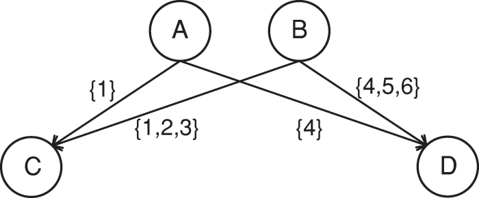
Figure 1: An example of two nodes communicating with their neighbors

However, the interaction behavior between nodes is not random, but is influenced by the node features reflected by their historical interaction behavior [4,5]. For instance, if two nodes have had frequent interactions in the past, they are likely to interact more frequently in the future. Furthermore, the historical interaction behavior between nodes also displays self-similarity, which mirrors the tendency of nodes to repeat their behaviors [6–8]. This behavior is reflected in the consistency of individual behavioral patterns across a time series. For example, if user A regularly contacts user B in the morning, they are likely to continue this pattern on subsequent mornings. Overall, the node features reflected in the historical interaction behaviors of nodes greatly influence information propagation. For example, in the real-time evolution of Twitter networks, researchers have found that the largest cascades tend to be generated by users with many followers and a large number of historical interaction behaviors [9].

Evidently, the node features embodied by these dynamic historical interaction behaviors are important in actual social networks, but are not adequately represented in traditional algorithms and propagation models of IM. The IM problem of temporal social networks faces the following challenges:

(1) Seed selection algorithms: traditional influence maximization algorithms have limited consideration of node characteristics in temporal social networks and cannot select high-quality seed nodes;

(2) Information propagation models: traditional information propagation models do not take into account the dynamic historical interaction behavior of nodes, and thus cannot be applied to temporal social networks.

Therefore, the motivation of this study is to more appropriately address the above issues in temporal social networks by considering the node features reflected by their historical interaction behaviors. Based on this, we first propose a voting-based IM algorithm called ISVoteRank. This algorithm initially determines the voting ability of each node based on its node features. During the voting process, voting weights are set based on the interaction strength between nodes, allowing nodes to vote for their in-neighbors at different extents, and subsequently weakening their voting ability accordingly. After the voting is completed, the top k nodes with the highest voting scores are selected as seed nodes. Subsequently, we designed an information propagation model called DIC, which utilizes the node features of interaction attributes and self-similarity to capture the dynamic features of temporal social networks, including dynamic changes in the activation time, activation probability, and activation frequency of nodes. In summary, our main contributions are as follows:

(1) We quantify the historical interaction behaviors of nodes into two node features, i.e., interaction attributes and self-similarity. To distinguish the order of interactions, we classify the interaction attributes into active interaction attributes and passive interaction attributes.

(2) We propose the node feature-aware voting algorithm ISVoteRank, which incorporates node features into the voting process, sets the node’s personalized initial voting ability, and dynamically adjusts the node’s voting ability in the voting process, allowing more efficient selection of seed nodes.

(3) We extend the traditional IC model to the DIC model, which combines the node features to set the activation time, activation probability, and activation frequency changes, so as to capture the dynamic features of the information propagation process.

(4) Experiments on four real-world temporal social network datasets demonstrate the superior performance of the ISVoteRank algorithm in terms of effectiveness and efficiency compared to existing baseline methods.

The remainder of this paper is organized as follows: Section 2 discusses related work. Preliminary definitions are introduced in Section 3. Section 4 describes the ISVoteRank algorithm for selecting seed nodes, and the DIC model for information propagation of seed nodes. Experimental results from real-world datasets are provided in Section 5, and Section 6 concludes the paper.

2  Related Works

In this section, a brief overview of related work on solutions to the influence maximization problem is provided, focusing on influence maximization algorithms and information propagation models.

2.1 Influence Maximization Algorithms

One of the main challenges of the IM problem lies in its complexity, which often makes direct calculation of the global optimum solution impractical. To address this issue, researchers have proposed many different algorithms. This section will focus on discussing three main categories: greedy algorithms, approximation algorithms, and heuristic algorithms.

Greedy algorithms offer a direct approach to the IM problem, choosing the best seed nodes by Monte Carlo simulations. Kempe et al. first proposed a greedy algorithm [10], which iteratively selects nodes that can maximize marginal influence to join the seed set. Greedy algorithms can guarantee that the obtained solution is over 63% of the global optimum, due to the submodular and monotonic properties of the IM problem. However, a major challenge of greedy algorithms lies in their computational complexity, particularly when a large number of simulations are required. Although greedy algorithms can provide (1-1/e) approximate solutions, their high computational complexity limits their application in large-scale networks.

Due to the computational complexity of greedy algorithms, many researchers have sought to design more efficient approximation algorithms. While approximation algorithms cannot guarantee finding the global optimum, they can find a relatively good solution within polynomial time. Leskovec et al. [11] proposed a Cost Effective Lazy Forward (CELF) algorithm, considering the cost and benefit of information spread in the network, achieving the effect of maximizing influence under a given budget. Chen et al. [12] proposed two improved greedy algorithms, called NewGreedy and MixedGreedy, which further optimize greedy algorithms by building subgraphs of the network. However, the complexity of these approximation algorithms remains high and can not be applied in large-scale social networks.

Heuristic algorithms are another approach to the IM problem. They rely on some strategy or heuristic information, aiming to find a relatively good solution without complex calculations [13–15]. These algorithms are particularly effective when dealing with large-scale networks. For example, Chen et al. [16] proposed a heuristic algorithm called DegreeDiscount, which considers a node’s degree and the influence of its neighboring nodes when selecting seed nodes. Zhang et al. [17] introduced the VoteRank algorithm, which identifies propagators in the network based on a voting mechanism. Subsequently, Sun et al. [18] extended VoteRank to weighted networks, proposing the WVoteRank algorithm. Kumar et al. [19] designed the NCVoteRank algorithm, considering the Neighborhood Coreness (NC) values of neighbors during voting. Later, Kumar et al. [20] took into account the weights of two-level neighbors, further improving the WVoteRank algorithm. Liu et al. [21] improved the VoteRank algorithm by combining the diversity of node voting capabilities, proposing the VoteRank++ algorithm. However, the above voting-based methods all select seeds by iteration, which can be time-consuming when the network size is large. In addition, the above methods only consider the node features in static social networks, resulting in only being applicable to static social networks and performing poorly in temporal social networks.

Recent studies have begun to focus on the IM problem in temporal social networks, and feature selection has become increasingly important [22–25]. For example, Wang et al. [26] introduced a pairwise factor graph (PFG) for simulating social influence, and a dynamic factor graph (DFG) to integrate temporal information. In addition, Zhang et al. [27] proposed an influence maximization framework, leveraging machine learning for prediction and replacement. Using past network snapshots, the framework predicts upcoming ones and identifies seed nodes suitable for dynamic networks based on these predictions. Chandran et al. [28] studied time influence maximization in dynamic social networks and proposed a seed selection method based on sliding windows.

From the above analysis, we note that for the IM problem in temporal social networks, most of the existing work addresses the problem through dynamic networks, such as sliding windows. This approach describes the evolution of the network through dynamic changes in the network, leading to a high time complexity. In conclusion, IM problems are complex and challenging, requiring a deep understanding of the network structure and node features.

2.2 Information Propagation Models

Information propagation models are the foundation of influence maximization research, used to simulate the process of information propagation in social networks. The two most common information propagation models are the IC model and the Linear Threshold (LT) model.

The IC model [10] is a probabilistic model that describes the process of information propagation in networks in a simple way. In this model, each activated node has one opportunity to activate its neighboring nodes. For any edge from an activated node to its neighbors, there is a fixed probability, indicating the possibility of the neighbor node being activated. However, the IC model mainly considers the global characteristics of the network and neglects the impact of individual node behavior, which may lead to errors when simulating the complex information propagation process in the real world. The LT model [10] is another commonly used information propagation model. In this model, each node is assigned a threshold. A node will be activated only when the number of activated nodes among its neighbors exceeds the threshold. Compared to the IC model, the LT model pays more attention to mutual influence between nodes, rather than just one-way influence. However, like the IC model, the LT model does not fully consider nodes’ individual behavior and dynamic characteristics. So these two models may have certain limitations when simulating the complex real-world information propagation process, especially in temporal social networks.

In addition to the IC and LT models, there are many other information propagation models being proposed, such as the Independent Cascade model on Temporal graph (ICT) [29], which modifies the IC model based on static graphs to enable information propagation on temporal graphs. Chen et al. [30] proposed the Improved Weighted Cascade Model (IWCM) in response to the problem that the Weighted Cascade Model (WCM) for static social networks does not apply to temporal social networks. Although these models take into account the temporal nature of information propagation, there are limitations such as ignoring the possibility of complex interactions between nodes and oversimplifying the complexity of information propagation.

Although current information propagation models have played an important role in understanding and simulating the propagation of information in social networks, their consideration factors are limited, especially the neglect of dynamic behavior and personalized characteristics of nodes, which may lead to certain limitations in complex real-world information propagation processes, especially for temporal social networks. Therefore, how to more comprehensively consider the diversity of networks in information propagation models, such as the dynamic behavior of nodes and complex interactions, is still an important direction of current studies, and is the problem this paper attempts to solve.

3  Preliminaries

This section introduces the relevant definitions of temporal social networks, and describes the node features reflected by their historical interaction behavior in this network.

3.1 Temporal Social Network

Definition 1: Temporal Social Network (TSN). We define a TSN as GT(V,E,TE), where V is the set of nodes, E is the set of edges, and TE is the time set corresponding to inter-node interactions. In this network, |V|=n and |E|=m. Interaction times between any two nodes u and v are represented by T(u,v), which is a subset of TE.

Distinct from conventional social networks, TSN incorporates the temporal sequence of interactions of nodes. As shown in Fig. 2, the edge values symbolize the interaction timestamps between users. For instance, given T(A,C)={1, 2}, if user A successfully activates user C at time 2, then C is active at and after time 2 and inactive before time 2. Subsequently, C may activate its neighbors D and E because C has interaction times with them at and after time 2. However, if B activates C at time 4, then C can only activate E since the interaction times between C and D are both before time 4. It is thus clear that the relationships between nodes in a TSN are not static, but dynamic over time.

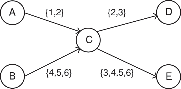
Figure 2: Temporal social network

Based on this analysis, a key feature of TSN is the interaction behavior between nodes, which reflects not only changes in network structure but also changes in node behavior. Therefore, it is important for the node characteristics reflected by the historical interaction behaviors of nodes.

3.2 Node Features

Based on the above analysis, this paper quantifies the node features reflected by their historical interaction behaviors as interaction attributes and self-similarity. Interaction attributes reflect the strength of node behavior in the past, while self-similarity reveals the time dependence of node behavior in the future.

3.2.1 Interaction Attributes

Definition 2: Interaction Attributes (IA). In a temporal social network, interaction attributes represent the interaction strength between a node and its neighbors.

Specifically, due to the importance of the temporal order of interactions in TSN, this paper categorizes IA into two types: active interacting attributes and passive interacting attributes.

Definition 3: Active Interaction Attribute (AIA). This attribute captures the proactive behavior of a node with its neighbors when initiating an interaction and reflects the node’s tendency to interact with its neighbors. Eq. (1) provides a method for calculating the AIA value of node v:

AIAv=∑w∈out(v)|T(v,w)|(1)

where |T(v,w)| represents the number of interactions from node v to node w, and out(v) denotes the set of out-neighbors of node v.

Definition 4: Passive Interaction Attribute (PIA): This attribute captures the receptive behavior of a node in response to an interaction initiated by its neighboring node and reflects the tendency of the node to be activated by its neighbors. Eq. (2) provides a method for calculating the PIA value of node v:

PIAv=∑u∈in(v)|T(u,v)|(2)

where |T(u,v)| represents the number of interactions from node u to node v, and in(v) denotes the set of in-neighbors of node v.

As shown in Fig. 2, node C has an AIA value of 6, while the PIA value is 5. By breaking down the AIA and PIA values of nodes, a better understanding and measurement of node interaction behavior patterns in temporal social networks can be achieved.

3.2.2 Self-Similarity

Definition 5: Self-similarity. Self-similarity reflects the fact that a node’s current behavior is influenced by the time series of its historical interaction behavior, describing the influence of past behavior on future behavior.

Crovella et al. [31] have highlighted the significance of self-similarity in the temporal sequences of node interactions. A common indicator to quantify the value of self-similarity in a time series is the Hurst index, which measures the autocorrelation of the time series [32,33]. The Hurst index values range from 0 to 1, indicating different trends [34]. When the Hurst index value ranges from 0 to 0.5, it indicates that the time series has anti-persistent properties. In this type of time series, high and low values alternate over the long term, showing a tendency to revert to the mean. When the Hurst index value equals 0.5, it indicates that the time series is random and uncorrelated. In this case, the correlation between current values and future values is negligible, making it difficult to identify clear trends. When the Hurst index value ranges from 0.5 to 1, it indicates that the time series has persistent properties. This means that a high value may trigger a series of high values that may persist for a long period in the future.

To evaluate the Hurst index, this study employs the rescaled range (R/S) analysis technique [34]. This statistical method is typically used to classify time series data and measure its variability over a specific time. For example, consider a scenario in a social network where user A has consistently posted daily status updates at 8 am over the past week. This behavior exhibits a phenomenon of self-similarity, suggesting a pattern or regularity in the timing of these updates. By applying the (R/S) method to quantify this behavior and calculating the value of the Hurst index, we can gain a deeper understanding of the persistence or long-term dependency of this activity. If the value of the Hurst index is close to 1, it means that the behavior of user A shows persistence. In other words, the presence of one high value (posting a daily status update at 8 am) tends to trigger a series of subsequent high values. This finding further emphasizes the potential self-similarity and predictability of user A’s past patterns over future patterns.

In summary, the interaction attributes and self-similarity reflect the historical interaction behavior of nodes, and enable a more precise understanding and analysis of node behavior. Interaction attributes reflect the strength of node behaviors in the past, and self-similarity reveals the temporal dependence of node behaviors in the future. These two features provide a mechanism to better identify influential nodes and predict their future behavior in complex and dynamic temporal social networks.

4  Proposed Methods

Based on the preliminary analysis, this paper proposes the ISVoteRank algorithm for selecting seed nodes, as well as the DIC information propagation model for estimating the influence spread of seed nodes. Fig. 3 shows the framework of our work.

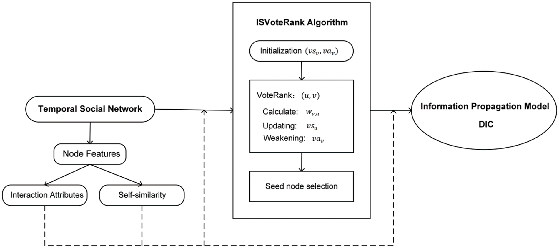
Figure 3: Working framework

As shown in Fig. 3, we proposed the ISVoteRank algorithm based on node features in temporal social networks. More specifically, the state of each node v is denoted as (vsv, vav), where vsv denotes the obtained voting score, and vav denotes the voting ability. For each directed edge (u,v), firstly, the voting weight wv,u from neighbor v to node u is computed, and secondly, the voting score of node u is updated and the voting ability of neighbor v is weakened. Finally, the top k nodes with the highest voting scores are selected as seed nodes. Subsequently, the selected seed nodes are simulated to propagate in the DIC information propagation model to estimate the influence spread of the seed nodes.

4.1 ISVoteRank Algorithm

In this section, we present the ISVoteRank algorithm, which is an extension of the VoteRank algorithm [17] that incorporates multidimensional optimization and improvements to better fit the specific characteristics of temporal social networks.

4.1.1 Initializing Voting Ability

In the original VoteRank algorithm [17], the initial voting ability of each node is set to 1. However, in temporal social networks, each node exhibits distinct characteristics, necessitating a personalized initialization of the voting ability.

According to the analysis in Section 3, the active interaction attribute reflects the node’s tendency to actively interact with its neighbors, and the self-similarity reflects the influence of the node’s past behavior on its future behavior. Therefore, here we combine these two features to set the initial voting capacity of the node, which is calculated as follows:

vav=hurst(v)+AIAvAIAmax(3)

where hurst(v) is the self-similarity of node v, AIAv is the value of the active interaction attribute of node v, and AIAmax is the value of the largest active interaction attribute in the whole network.

4.1.2 Computing Voting Score

In static social networks, the voting weights of nodes are shown in Fig. 4a, and the VoteRank strategy [17] assumes that each node has the same voting weight for all its neighbors. However, in temporal social networks, as shown in Fig. 4b, different interaction strengths among nodes should lead to different voting weights among nodes.

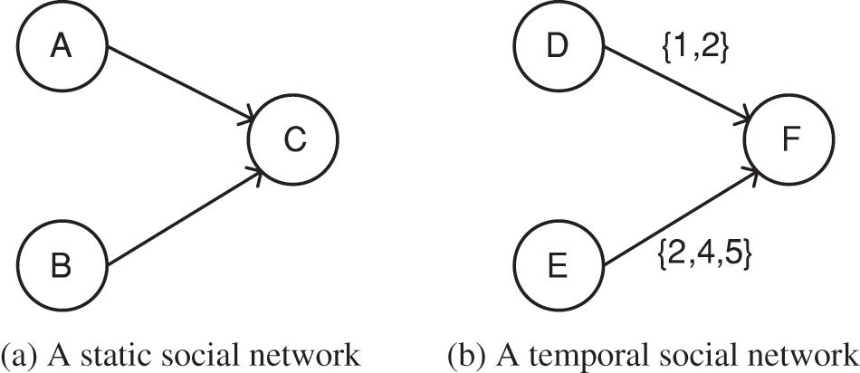
Figure 4: Comparison of voting weights

Therefore to address this problem, this paper overcomes this limitation by introducing personalized voting weights based on node features. As shown in Fig. 4b, the voting weight from node D to node F depends on a ratio, i.e., the number of node F’s passive interactions with node D to the number of node F’s passive interactions with all its neighbors. Therefore, the voting weight of node v for its neighbor u is given by Eq. (4):

wv,u=|Tu,v|PIAv(4)

where |T(u,v)| represents the number of interactions from node u to node v, and PIAv denotes the Passive Interaction Attribute of node v.

Based on Eq. (4), the voting score of node u is further defined as follows:

vsu=∑v∈outuwv,uvav(5)

where wv,u denotes the weight that node v gives to node u to vote, vav denotes the voting ability of node v, and outu denotes the set of out neighbors of node u.

4.1.3 Weakening Voting Ability

In VoteRank [17], seed nodes are selected through iterative voting. Once a seed is selected, its voting ability is set to 0, and the voting ability of its neighboring nodes is weakened. These settings are implemented to prevent an excessive concentration of identified influential nodes in the network. However, this iterative approach may be less efficient when applied to large-scale social networks. To address this limitation, the ISVoteRank algorithm introduces a new mechanism. Once a node completes voting for its neighbors, its voting capacity is reduced based on specific rules. When a node’s voting capacity reaches 0, it no longer participates in the following voting process. This design aims to overcome the drawbacks of iterative voting and also prevents excessive concentration of seed nodes. Specifically, after node v votes for node u, the voting capacity of node v is weakened according to Eq. (6):

vav={vav−δ,if vav−δ>0 0,otherwise(6)

where

δ=wv,u∗1AIAavg(7)

where AIAavg is the average active interaction attribute value of the nodes in the network.

4.1.4 Selecting Seed Nodes

Based on the above analysis, to reduce the aggregation of the selected seed nodes, the voting ability is dynamically adjusted by combining the node features during the voting process. Therefore, in the seed selection phase, the top k nodes with the highest voting scores can be sequentially selected as seed nodes after one voting process. As shown in Eq. (8):

S={u|u=[ui|ui∈GT,vsui>vs′,i∈{1,…,n}]}(8)

where S represents the set of seed nodes, ui is a node in GT, vsui denotes the voting score of ui, and vs′ is the k+1th higher vs value of nodes in GT.

4.1.5 Algorithm Process

The voting process of ISVoteRank is outlined in Algorithm 1. Initially, the algorithm initializes the voting ability and score for each node in the network (lines 3–4). It then proceeds to iterate through each edge (u,v) (line 6). During this iteration, if the voting ability of node v is greater than 0, indicating it has the ability to vote, the algorithm calculates the weight of node v to vote for node u (line 8). Subsequently, it updates the voting score of node u and adjusts the voting ability of node v (lines 9–10). Finally, the algorithm selects the top k nodes with the highest scores and adds them to the seed node set S (line 13). Following this process, ISVoteRank ensures that each node’s voting ability and score are appropriately initialized, and dynamically adjusted based on their participation in the voting process.

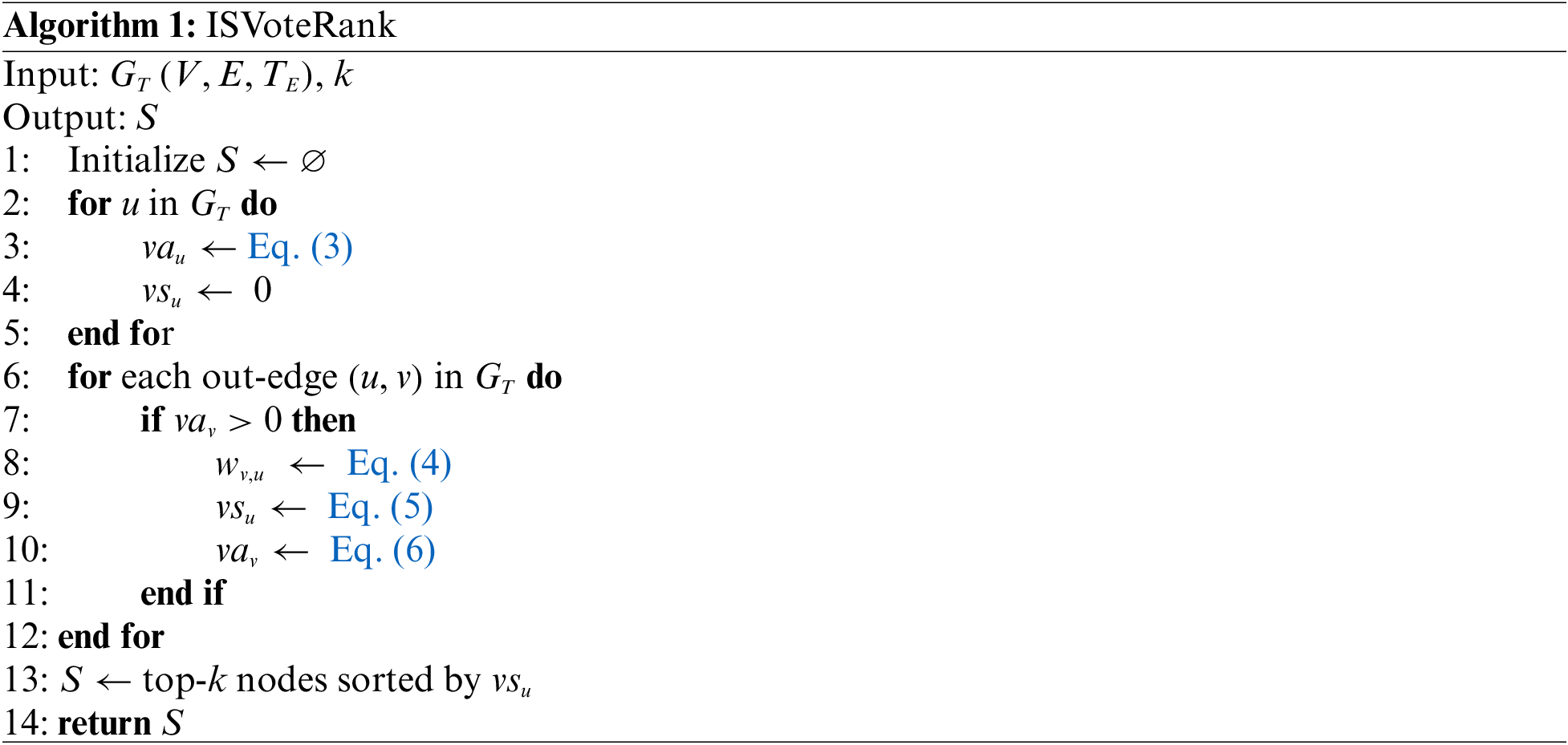
The complexity analysis of ISVoteRank can be divided into three steps. In the initialization phase (lines 2–5), the algorithm traverses all nodes, resulting in a time complexity of O(n), where n is the number of nodes. During the voting phase (lines 6–12), the algorithm traverses all edges, resulting in a time complexity of O(m), where m is the number of edges. The seed selection phase (line 13) involves sorting all nodes based on their scores. This step has a time complexity of O(nlogn), where n is the number of nodes. Overall, the total time complexity of the ISVoteRank algorithm can be approximated as O(n + m + nlogn) or more concisely expressed as O(m + nlogn).

It can be seen that the ISVoteRank algorithm effectively combines voting weights with the voting process, avoiding the drawbacks of iterative voting in traditional voting algorithms, and has relatively low time complexity, making it computationally efficient when dealing with large-scale temporal social networks.

4.2 Dynamic Independent Cascade Model

The traditional IC model has been widely utilized in analyzing information propagation within static social networks. However, when applied to temporal social networks, the limitations of the IC model become apparent as it fails to effectively capture the dynamic features of such networks. This is primarily because the IC model assumes static network connectivity patterns, where an active node has only one chance to activate each of its inactive neighbor nodes, and the activation process does not take into account the temporal sequence of node interactions. In contrast, real social networks exhibit dynamic changes in connectivity.

To address this problem, this paper proposes a dynamic independent cascade model, called the DIC model. This model incorporates node features reflected by their historical interaction behavior into the DIC model for capturing the dynamic features of the temporal social network. These dynamic features include changes in node activation times, activation probabilities, and activation frequencies. Specifically, activation time is related to the evolution of historical interaction time, activation probability is related to interaction attributes and varies with activation frequency, and activation frequency is influenced by the self-similarity observed in the historical interaction behavior of nodes. By integrating these factors, this model can capture changes in node behaviors based on node features, thus capturing the dynamic characteristics of the temporal social network.

4.2.1 Activation Time

Definition 6: Activation Time. The moment when node v is successfully activated by its active parent node u is its activation time, denoted as Actv={t|t∈T(u,v) and t≥Actu}.

The IM algorithm for static social networks does not need to consider the activation time of the node, while the time when the node is successfully activated in a temporal social network needs to be considered, and the activation time of the node will change as the node interaction behaviors occur. As shown in Fig. 5, node B is selected as the seed node with the initial activation time set to 0, and the rest of the nodes have their initial activation time set to −1. When node B successfully activates node C at moment 4, the activation time of node C will be updated to 4.

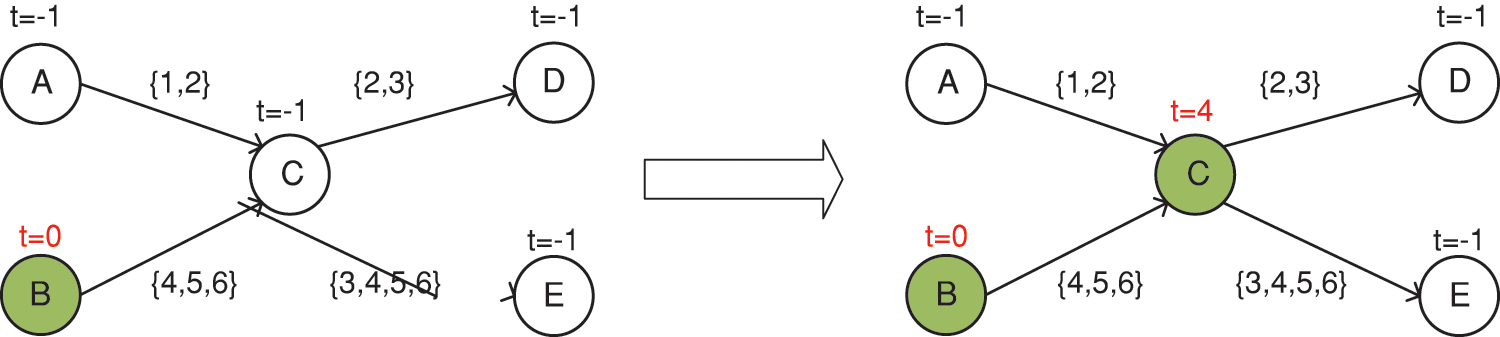
Figure 5: Variation in activation time during information propagation

4.2.2 Activation Probability and Activation Frequency

In static social networks, as in Fig. 6a, active node A activates its inactive neighbor nodes B and C with the same probability and only one activation opportunity. However, in temporal social networks, as in Fig. 6b, the difference in interaction strength between nodes results in different probabilities for active node D to activate its inactive neighbor nodes E and F.

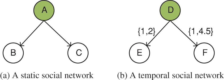
Figure 6: Comparison of activation probability and activation frequency in different social networks

Therefore, to capture the dynamics of the information propagation process, we first set the activation probability in combination with the interaction attributes of the nodes. Then, when the first activation fails but there is still interaction behavior, we judge the activation frequency based on the self-similarity of the inactivated nodes, i.e., the Hurst index of an inactivated node is greater than 0.5, which represents the possibility of interaction behavior of the node, and thus activation is performed again. Detailed definitions of activation frequency and activation probability are shown below:

Definition 7: Activation Frequency. Activation frequency is a measure of the number of times a node is activated during the propagation of information.

Definition 8: Activation Probability. Activation probability is the probability that an inactive node v is successfully influenced by its active parent node u through the directed edge (u,v), denoted as Pu,v∗∈[0,1].

In static social networks, degree estimation is usually used to calculate the activation probability between nodes. However, in temporal social networks, there are different interaction behaviors among nodes, which implies the dynamics of activation probabilities among nodes. Therefore, in this paper, the activation probability is defined by Eq. (9):

Pu,v∗=1−(1−Pu,v)θ, s.t. θ ∈ [1, |T(u,v)|](9)

where

Pu,v=|T(u,v)|PIAv(10)

where Pu,v denotes the probability of node u activating node v for the first time, PIAv denotes the passive interaction attribute of node v, and |T(u,v)| denotes the number of interactions from node u to node v. θ denotes activation frequency. The activation probability increases with the increase of activation frequency.

4.2.3 Information Propagation Process

In the DIC model, initially, all nodes v in the network except the seed node are set to be inactive, i.e., their initial activation time Actv= −1. When a seed node u is selected to start influence propagation, the following process is set:

(1) Let the initial activation time of the seed node be Actu=0, i.e., the seed node u is active at the time moment 0. At this time, u activates its inactive neighbor node v with a certain probability, and u has at least one chance to try to activate v.

(2) When u tries to activate v, the interaction times between nodes are traversed sequentially, if the condition Actu={t|t∈T(u,v) and Actu≤t} is satisfied, u activates v with probability Pu,v∗.

(3) If u fails to activate v for the first time, the self-similarity of v is calculated and if hurst(v)>0.5, activation of v will be attempted again until all interaction times have been traversed.

(4) If v is successfully activated by u at the time moment t={t|t∈T(u,v)}, its activation time Actv is recorded, where Actv=t.

(5) The influence propagation process stops when all active nodes have tried to activate their neighbors and no new nodes have been activated.

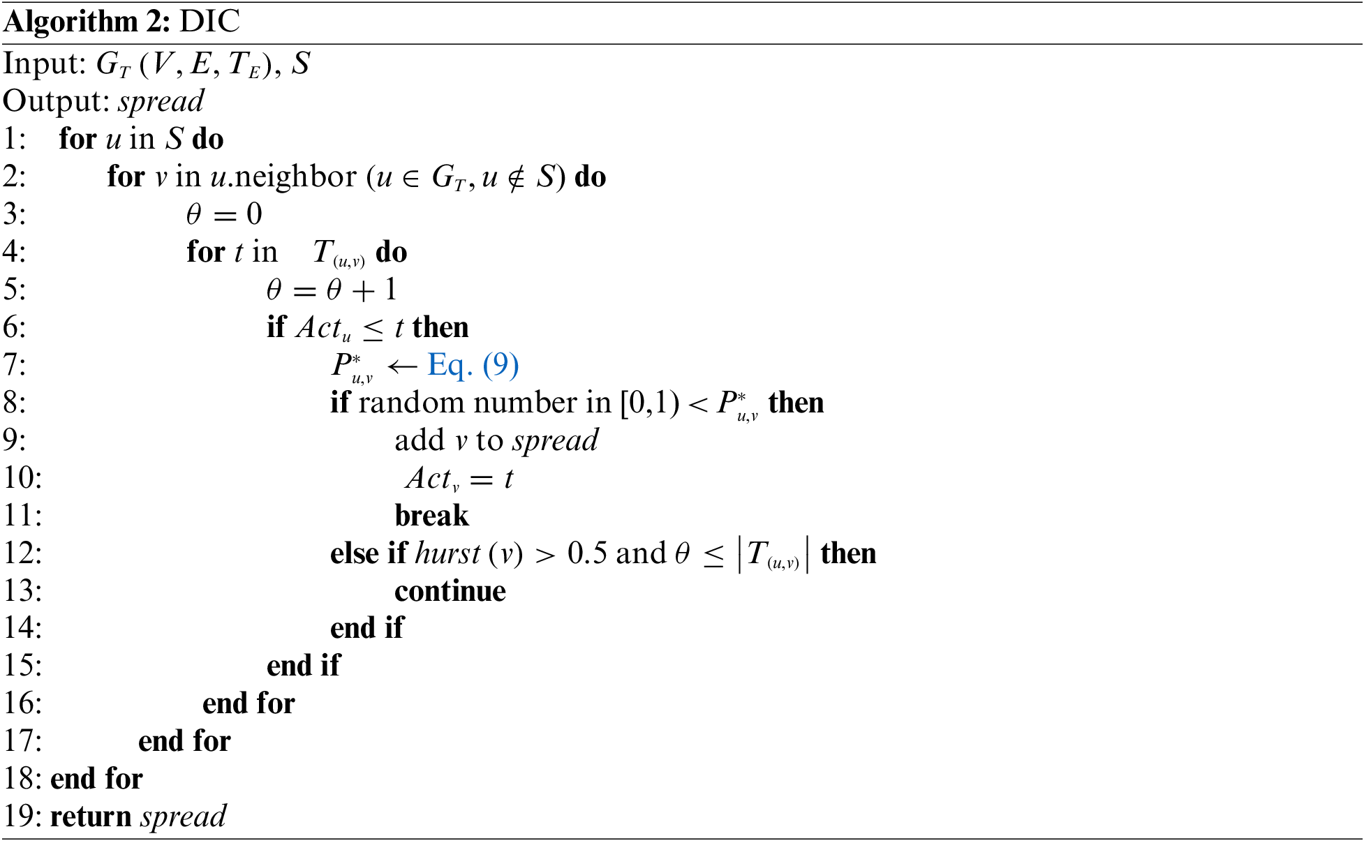
Algorithm 2 illustrates the propagation process of the DIC model mentioned above. We can see that the DIC model offers an effective approach to capturing the dynamic features of the temporal social networks by considering node features revealed by the historical interaction behaviors during information propagation.

5  Experiments

5.1 Experimental Settings

5.1.1 Data

We utilized four real-world datasets from SNAP, available at http://snap.stanford.edu/data/. Each row in these datasets contains three components represented as (u,v,t), which signifies an interaction between u and v at time t. The comprehensive details of these datasets can be found in Table 1.

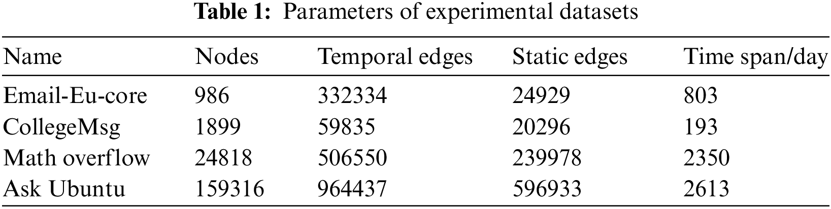
Dataset 1 [35] is based on email data from a European research institution. Dataset 2 [36] captures private messages from a University of California online network. Dataset 3 [35] and Dataset 4 [35] represent user interactions on Math Overflow and Ask Ubuntu, respectively.

5.1.2 Baseline Methods

Seven methods are used as baselines, which are related to voting mechanisms and other heuristics. They are described as follows:

VoteRank [17]: As a basic voting algorithm, VoteRank sets the initial voting ability of the node to 1, and then selects the node with the highest score as the seed node through iterative voting.

WVoteRank [18]: WVoteRank is an extension of VoteRank, which incorporates the edge weights related to the node’s nearest neighbors (one-hop neighbors) into the calculation of voting scores, and iteratively votes to select the node with the highest score as the seed node.

NCVoteRank [19]: NCVoteRank incorporates the Neighborhood Coreness (NC) value of a node into the calculation of its voting score, and then selects the node with the highest score as the seed node through iterative voting.

VoteRank++ [21]: Based on the basic principles of VoteRank, VoteRank++ improves the initial voting ability of nodes and the calculation of voting scores. Although the seed selection strategy is improved, it still cannot guarantee good time performance.

K_shell [37]: K_shell is a method for determining the centrality of a network node by calculating the K_shell value (or Ks value) of each node to determine the importance of the node.

DegreeDiscount [16]: DegreeDiscount is a seed node selection method based on the degree of a node. The core idea is that when a node v’s neighboring nodes are selected as seed nodes, the degree of node v is discounted to reduce its influence in subsequent seed selection.

Max_activity: This algorithm selects the top k nodes with the highest value of AIA as seed nodes in this paper.

5.1.3 Parameter Settings and Preprocessing

Parameter settings: To compare the impact of these different methods on the same dataset, all algorithms run 1000 Monte Carlo simulations in the DIC model, and take the average influence spread value as the final result, so the observed differences are statistically significant. The activation probability is set as shown in Section 4.1.3. The range of the seed number is set between 10 and 100.

Preprocessing: For the ISVoteRank algorithm, the Hurst index value, representing nodes’ self-similarity, is computed offline based on the nodes’ interaction time series. This preprocessing step is necessary for efficiently calculating the Hurst index values.

5.2 Experimental Results

Our experiments are divided into three parts:

(1) Influence spread: comparing the effectiveness of algorithms by propagating the seed nodes’ influence selected by algorithms through the DIC model, and comparing the differences between the DIC and IC models by propagating the seed nodes’ influence selected by the ISVoteRank algorithm;

(2) Time performance: comparing the efficiency of algorithms by comparing the running time variation of algorithms in selecting 10 to 100 seed nodes;

(3) Average shortest path length: by comparing the average shortest distance length between the seed nodes selected by algorithms, thus verifying that the algorithm proposed in this paper does not perform iterative seed selection but still reduces the aggregation of seed nodes.

5.2.1 Influence Spread

Firstly, to observe the effectiveness of the algorithms, we calculate the influence spread of different algorithms by varying the number of seeds from 10 to 100. The experimental results are shown in Fig. 7.

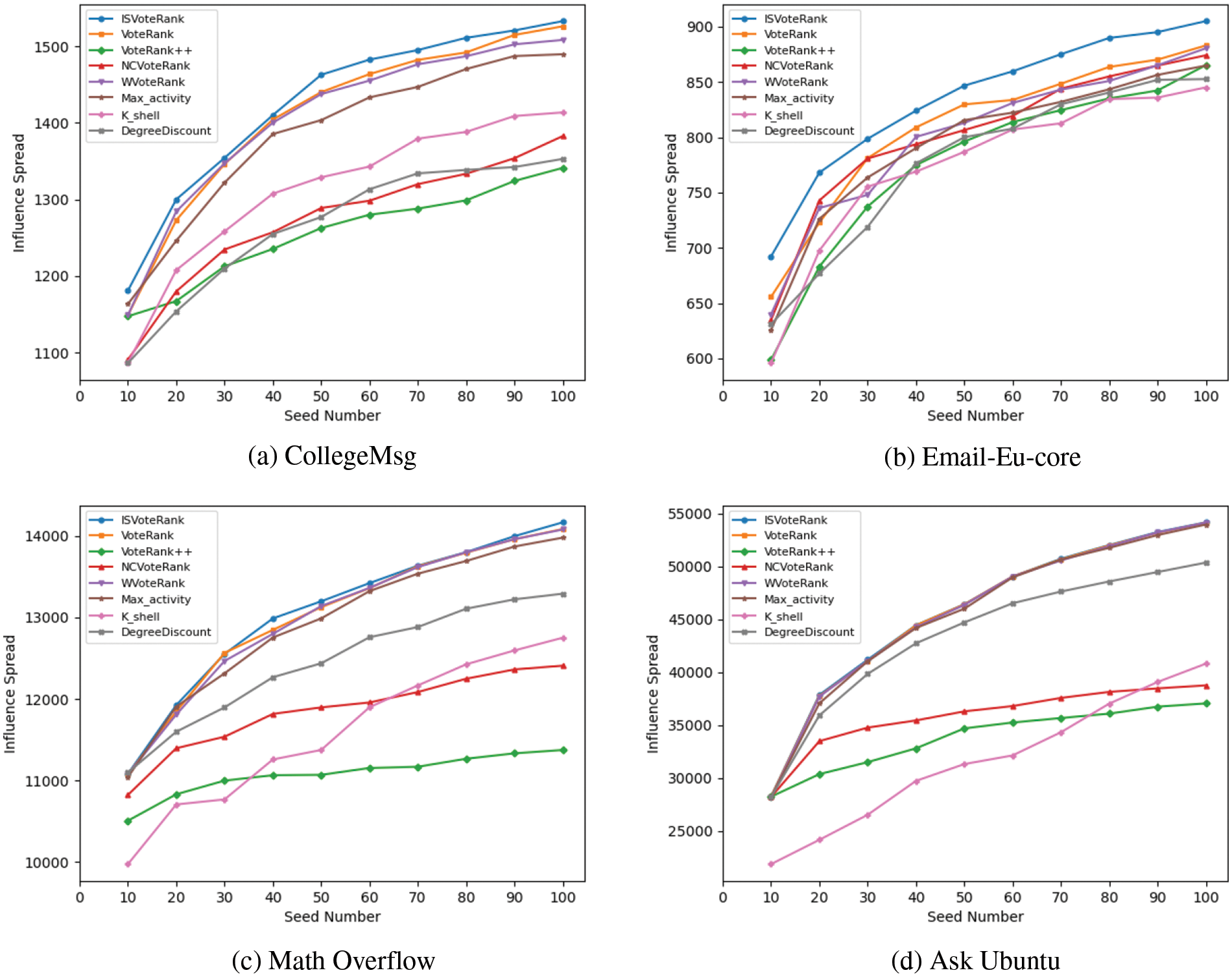
Figure 7: The influence spread of different algorithms varies with the number of seeds

From the figure, it is worth noting that the ISVoteRank algorithm achieves a relatively higher influence spread on all of the datasets. E.g., in Fig. 7a, when the k = 50, ISVoteRank reaches an influence of about 1462.78, while the closest VoteRank is about 1430.12 and the worst VoteRank++ is about 1262.56, which means ISVoteRank improves by approximately 2.28% compared to the closest algorithm and approximately 15.88% compared to the worst algorithm. More precisely, in Fig. 7a, when the number of seeds is 40 to 80, ISVoteRank outperforms the next best VoteRank by about 1.2%, and as the number of seeds increases, ISVoteRank and VoteRank gradually get closer, but ISVoteRank still ranks first. It is closely followed by WVoteRank and the Max_activity, while K_shell, NCVoteRank, DegreeDiscount and VoteRank++ underperform. In Fig. 7b, ISVoteRank outperforms the rest algorithms in terms of effectiveness as the number of seeds increases. In Fig. 7c, ISVoteRank is relatively better, followed by VoteRank, WVoteRank, and Max_activity. The rest of the algorithms perform worse. In Fig. 7d, ISVoteRank performs comparable to the VoteRank, WVoteRank, and Max_activity, followed by DegreeDiscount, and the rest of the algorithms are relatively poor. In addition, it is seen that VoteRank++ performs worse compared to the other voting algorithms in all datasets. The reason is that VoteRank++ considers more features of static social networks to improve voting ability, making it less suitable for temporal social networks.

The above phenomenon can be explained as follows. First, ISVoterank, VoteRank, WVoteRank, NCVoteRank and VoteRank++ are all voting strategy-based algorithms. However, VoteRank, WVoteRank, NCVoteRank and VoteRank++ only consider the static features of the network and ignore the node features reflected by their historical interaction behavior, which leads to poor results. Secondly, ISVoteRank uses the interaction strength between nodes to set personalized voting weights, which is very helpful in improving the effectiveness. Finally, when weakening the voting ability of nodes, ISVoteRank also weakens the voting ability differently according to the interaction strength between nodes, which is more in line with the interaction behavior of nodes. Overall, ISVoteRank performs well, reflecting its effectiveness in the face of complex temporal social networks.

Subsequently, we compare the influence spread of ISVoteRank in DIC and IC information propagation models. Since the ISVoteRank algorithm shows robust performance in the above experiments. Therefore, we first run the ISVoteRank algorithm to generate a seed set of k = 50, and then use the seed set as an input to the DIC and IC propagation models, respectively. The results are shown in Fig. 8. IC_ISVoteRank means the ISVoteRank algorithm runs in the IC model and the DIC_ISVoteRank means the ISVoteRank algorithm runs in the DIC model.

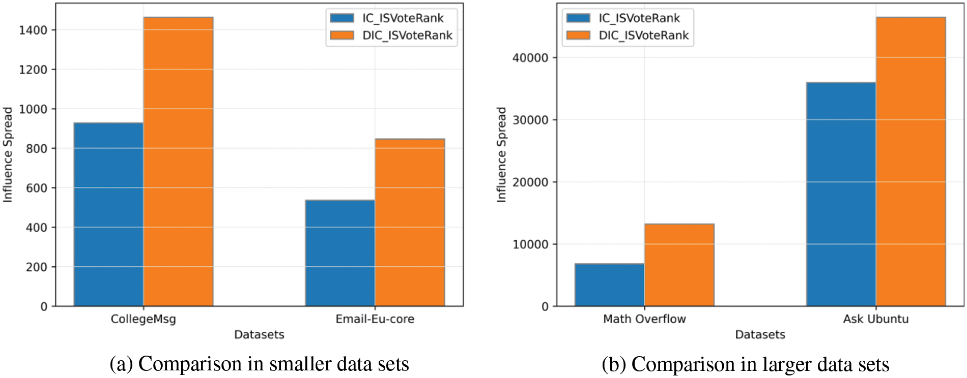
Figure 8: Comparison of influence spread of the VoteRank algorithm in different models

From the figure, we observe that when the data set is small, as in Fig. 8a, the influence spread of seeds in the DIC model is about twice as much as that in the IC model; when the data set is large, as shown in Fig. 8b, the DIC model still performs better than the IC model. From these results, the DIC model shows a stronger information propagation ability due to its combination of node features in temporal social networks.

5.2.2 Time Performance

In this section, we compare the efficiency of different algorithms. First, when k = 50, we count the running time of each algorithm on different datasets, and the results are shown in Table 2. Secondly, we vary the seeds from k = 10 to k = 100, and count the running time of different algorithms varies with the number of seeds. Fig. 9 shows the results in the form of a box plot. The abscissa represents different algorithms, and the ordinate records the running time of the corresponding algorithm.

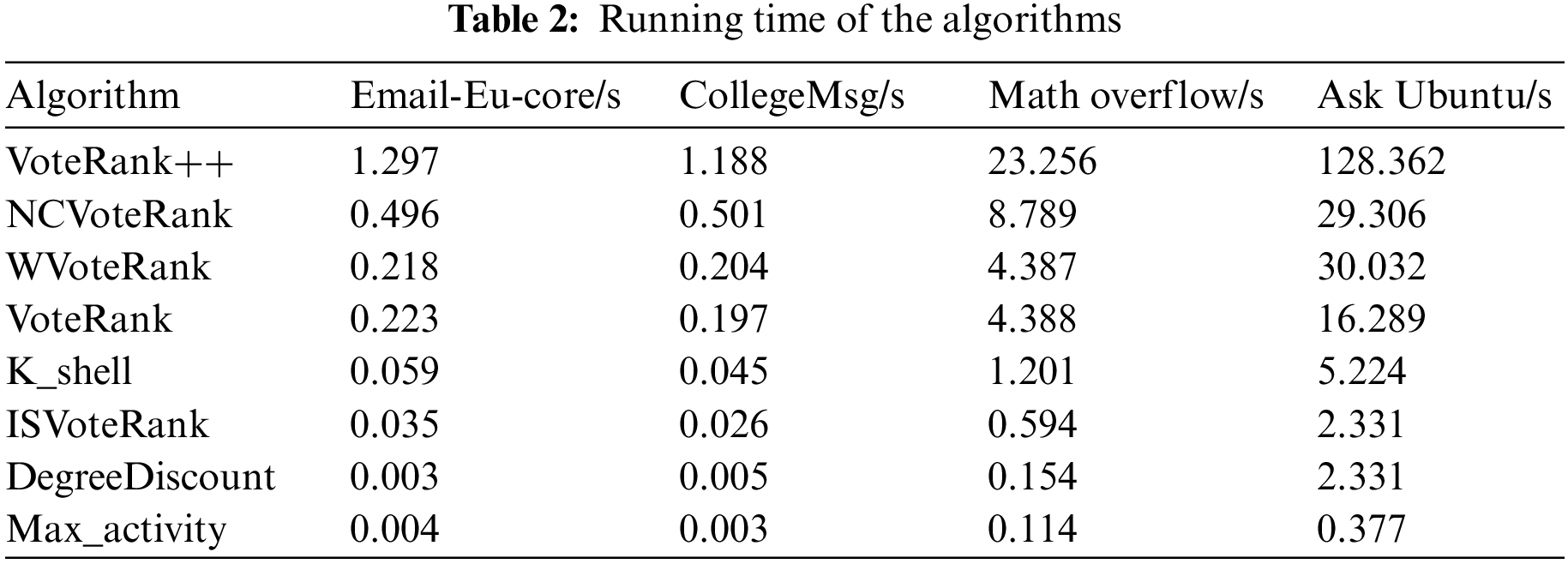
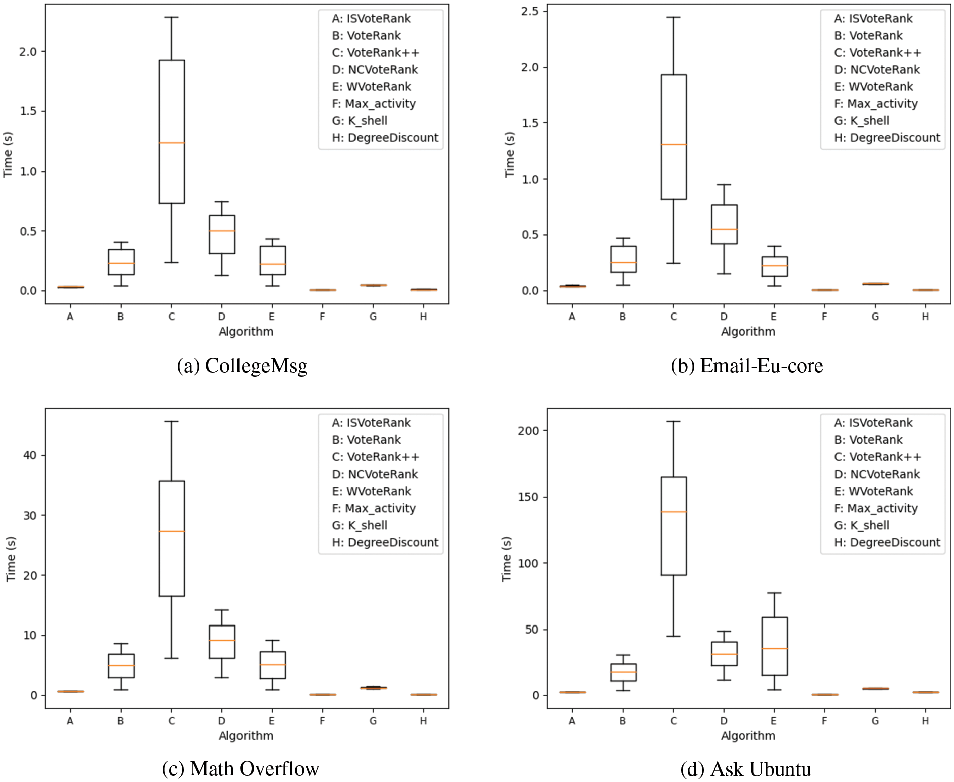
Figure 9: The running time of different algorithms varies with the number of seeds

From Table 2, we get the following observations: First, ISVoteRank is more efficient compared to voting-based algorithms. Among them, ISVoteRank is about 0.18, 0.15, 3.79 and 13.95 s faster than VoteRank in four data sets. This means that as the network size increases, the running time of ISVoteRank increases less. This is because the ISVoteRank algorithm does not need to iteratively vote to select seeds, and only votes once to select seed nodes. Secondly, compared with other non-voting algorithms, although ISVoteRank is not as good as DegreeDiscount and Max_activity, in Section 5.2.1, ISVoteRank’s influence spread is better than these two algorithms.

From Fig. 9, it can be seen that ISVoteRank proposed in this paper has a significantly shorter running time compared with other voting-based algorithms, and the running time fluctuations for different numbers of seeds are small, reflecting its efficiency and stability. In addition, the running time of Max_activity, K_shell, and DegreeDiscount are also shorter and comparable to ISVoteRank, and the runtime fluctuations are relatively small, showing excellent stability.

The above phenomena can be explained as follows. First, ISVoteRank avoids the drawback of iterative seed selection in traditional voting algorithms and can select seeds quickly. While the rest of the voting-based algorithms belong to the traditional voting algorithms, the iterative selection of seed nodes takes more time. In particular, VoteRank++ takes more factors into account leading to a long running time, especially in larger datasets, such as Fig. 9d, the average running time of the VoteRank++ reaches about 140 s. Second, the Max_activity, K_shell, and DegreeDiscount only consider a certain feature of the nodes. Although their running time is shorter, they cannot guarantee the performance of the influence spread as can be seen from Fig. 7. In summary, Fig. 9 vividly reveals the advantages of ISVoteRank in terms of running efficiency and stability.

5.2.3 Average Shortest Path Length

As highlighted in [17], the distance between seeds plays a crucial role in maximizing influence. When the identified seeds are widely distributed in the network, they tend to exert influence over a larger range of nodes. Therefore, the average shortest path length between seeds, denoted as Ls, is used as an indicator to evaluate the spread of seeds’ influence. A larger value of Ls indicates that the selected seeds are more dispersed and have a broader range of influence. The formula of Ls is provided in Eq. (11):

Ls=1|S|(|S|−1)∑u,v∈S,u≠vluv(11)

where S is a set of identified seeds and luv denotes the length of the shortest path from node u to node v.

As shown in Fig. 10, ISVoteRank outperforms VoteRank, WVoteRank, and DegreeDiscount in terms of Ls values in each dataset. This indicates that the influential nodes selected by ISVoteRank are more dispersed in the network, further reflecting the reasonableness of the voting strategy designed in this paper. Although VoteRank++ and NCVoteRank perform reasonably well in each dataset, it is worth noting that they do not perform well in terms of influence spread because the average distance between the seed nodes selected by these algorithms is too large. While the K_shell algorithm performs better only in Fig. 10a, Max_activity performs better only in Fig. 10b. In contrast, ISVoteRank proposed in this paper is more stable.

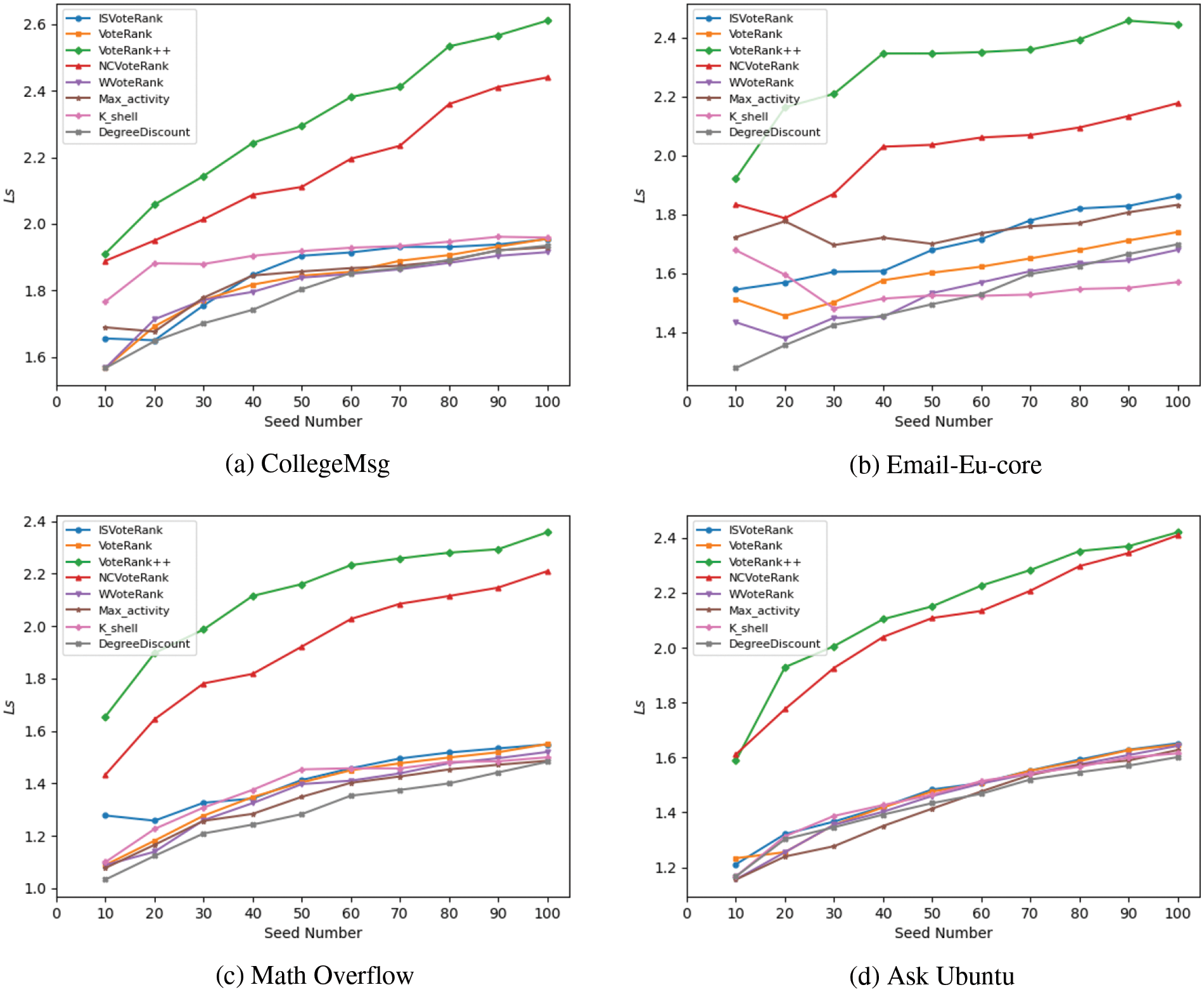
Figure 10: The average shortest path length of seeds selected by different algorithms varies with the number of seeds

The above phenomenon can be explained as follows. On the one hand, ISVoteRank sets the voting weights according to the interaction strength between nodes during the voting process, which can make the neighbors obtain different degrees of voting scores. On the other hand, once a node votes, it weakens the node’s voting ability according to the voting weight, and this strategy further distinguishes the voting scores obtained by neighbors. Combining the above strategies, the voting algorithm proposed in this paper reduces the aggregation of seed nodes.

5.2.4 Results Analysis

From the above experiments, it can be seen that ISVoteRank proposed in this paper obtains good performance in terms of effectiveness and efficiency, and these results are further analyzed next.

First, in terms of influence spread, i.e., effectiveness, ISVoteRank performs well, although VoteRank and WVoteRank also perform well in Figs. 7c and 7d, their failure to consider the node features of the temporal social network leads to poor results in other datasets. Second, in terms of time performance, i.e., efficiency, ISVoteRank avoids the drawback of iterative seed node selection, leading to a much better time performance than other voting-based algorithms, on par with Max_activity, K_shell, and DegreeDiscount. Third, the experimental results of the average shortest path length of seed nodes further reflect that although ISVoteRank only selects seed nodes at once, the design of the algorithm in the voting process still reduces the aggregation of seed nodes, no less than VoteRank. Overall, ISVoteRank performs well for considering node features reflected by their historical interaction behavior and the optimization of the voting process. These results reflect the superiority of ISVoteRank, which provides an effective and efficient solution to the IM problem in temporal social networks.

6  Conclusion

In conclusion, this study presents an innovative approach to the IM problem within temporal social networks by incorporating node features, specifically interaction attributes and self-similarity derived from nodes’ historical interaction behavior. This incorporation has led to the proposition of the node-feature-aware voting algorithm ISVoteRank and the DIC model. The ISVoteRank algorithm optimizes the voting mechanism by using node features, avoiding the inefficient iterative strategy of traditional voting-based algorithms, and allowing the algorithm to efficiently select high-quality seed nodes. The DIC model captures the dynamic changes of node activation time, activation probability and activation frequency during information propagation. Experiments on four real-world temporal social network datasets demonstrate that ISVoteRank has superior performance in terms of efficiency and effectiveness compared to existing baseline methods. Overall, this research offers a practical and innovative solution to the IM problem in temporal social networks. However, it is worth noting that this work has some limitations, such as limited consideration of the community structure of social networks. Since the community structure reflects more intensive interaction patterns among users, users in the same community often have similar interests and opinions, which will inevitably affect the speed and scope of information propagation. In view of this consideration, in future research work, we will further explore temporal social networks more deeply in combination with community structure to enhance the robustness and applicability of the proposed models and algorithms.

Acknowledgement: Not applicable.

Funding Statement: This work is supported by the Fundamental Research Funds for the Universities of Heilongjiang (Nos. 145109217, 135509234), the Youth Science and Technology Innovation Personnel Training Project of Heilongjiang (No. UNPYSCT-2020072), and the Innovative Research Projects for Postgraduates of Qiqihar University (No. YJSCX2022048).

Author Contributions: Study conception and design: W. Zhu, Y. Miao; data collection: Y. Miao, S. Yang; analysis and interpretation of results: Y. Miao, Z. Lian, L. Cui; draft manuscript preparation: W. Zhu, Y. Miao. All authors reviewed the results and approved the final version of the manuscript.

Availability of Data and Materials: All of the datasets used are available at http://snap.stanford.edu/data/.

Conflicts of Interest: The authors declare that they have no conflicts of interest to report regarding the present study.

References

1. S. S. Singh, D. Srivastva, M. Verma and J. Singh, “Influence maximization frameworks, performance, challenges and directions on social network: A theoretical study,” Journal of King Saud University-Computer and Information Sciences, vol. 34, no. 9, pp. 7570–7603, 2022. [Google Scholar]

2. F. Kazemzadeh, A. A. Safaei and M. Mirzarezaee, “Influence maximization in social networks using effective community detection,” Physica A: Statistical Mechanics and its Applications, vol. 598, pp. 127314, 2022. [Google Scholar]

3. S. Banerjee, M. Jenamani and D. K. Pratihar, “A survey on influence maximization in a social network,” Knowledge and Information Systems, vol. 62, pp. 3417–3455, 2020. [Google Scholar]

4. C. Fan, J. L. Guo and Y. L. Zha, “Fractal analysis on human behaviors dynamics,” arXiv preprint arXiv:1012.4088, 2010. [Google Scholar]

5. B. Fu, J. Zhang, H. Bai, Y. Yang and Y. He, “An influence maximization algorithm for dynamic social networks based on effective links,” Entropy, vol. 24, no. 7, pp. 904, 2022. [Google Scholar] [PubMed]

6. Q. Liu, X. Zhao, W. Willinger, X. Wang, B. Y. Zhao et al., “Self-similarity in social network dynamics,” ACM Transactions on Modeling and Performance Evaluation of Computing Systems (TOMPECS), vol. 2, no. 1, pp. 1–26, 2016. [Google Scholar]

7. B. Saxena and V. Saxena, “Hurst exponent based approach for influence maximization in social networks,” Journal of King Saud University-Computer and Information Sciences, vol. 34, no. 5, pp. 2218–2230, 2022. [Google Scholar]

8. W. Wang, S. Shi and X. Fu, “The subnetwork investigation of scale-free networks based on the self-similarity,” Chaos, Solitons & Fractals, vol. 161, pp. 112140, 2022. [Google Scholar]

9. E. Bakshy, J. M. Hofman, W. A. Mason and D. J. Watts, “Everyone’s an influencer: Quantifying influence on twitter,” in Proc. of the 4th ACM Int. Conf. on Web Search and Data Mining, New York, NY, USA, pp. 65–74, 2011. [Google Scholar]

10. D. Kempe, J. Kleinberg and É. Tardos, “Maximizing the spread of influence through a social network,” in Proc. of the 9th ACM SIGKDD Int. Conf. on Knowledge Discovery and Data Mining, New York, NY, USA, pp. 137–146, 2003. [Google Scholar]

11. J. Leskovec, A. Krause, C. Guestrin, C. Faloutsos, J. VanBriesen et al., “Cost-effective outbreak detection in networks,” in Proc. of the 13th ACM SIGKDD Int. Conf. on Knowledge Discovery and Data Mining, New York, NY, USA, pp. 420–429, 2007. [Google Scholar]

12. W. Chen, Y. Wang and S. Yang, “Efficient influence maximization in social networks,” in Proc. of the 15th ACM SIGKDD Int. Conf. on Knowledge Discovery and Data Mining, New York, NY, USA, pp. 199–208, 2009. [Google Scholar]

13. Y. Hua, B. Chen, Y. Yuan, G. Zhu and J. Ma, “An influence maximization algorithm based on the mixed importance of nodes,” Computers, Materials & Continua, vol. 59, no. 2, pp. 517–531, 2019. [Google Scholar]

14. C. Guo, L. Yang, X. Chen, D. Chen, H. Gao et al., “Influential nodes identification in complex networks via information entropy,” Entropy, vol. 22, no. 2, pp. 242, 2020. [Google Scholar] [PubMed]

15. Q. Li, L. Cheng, W. Wang, X. Li, S. Li et al., “Influence maximization through exploring structural information,” Applied Mathematics and Computation, vol. 442, pp. 127721, 2023. [Google Scholar]

16. W. Chen, C. Wang and Y. Wang, “Scalable influence maximization for prevalent viral marketing in large-scale social networks,” in Proc. of the 16th ACM SIGKDD Int. Conf. on Knowledge Discovery and Data Mining, New York, NY, USA, pp. 1029–1038, 2010. [Google Scholar]

17. J. X. Zhang, D. B. Chen, Q. Dong and Z. D. Zhao, “Identifying a set of influential spreaders in complex networks,” Scientific Reports, vol. 6, no. 1, pp. 27823, 2016. [Google Scholar] [PubMed]

18. H. L. Sun, D. B. Chen, J. L. He and E. Ch’ng, “A voting approach to uncover multiple influential spreaders on weighted networks,” Physica A: Statistical Mechanics and its Applications, vol. 519, pp. 303–312, 2019. [Google Scholar]

19. S. Kumar and B. S. Panda, “Identifying influential nodes in social networks: Neighborhood coreness based voting approach,” Physica A: Statistical Mechanics and its Applications, vol. 533, pp. 124215, 2020. [Google Scholar]

20. S. Kumar and A. Panda, “Identifying influential nodes in weighted complex networks using an improved WVoteRank approach,” Applied Intelligence, vol. 52, no. 2, pp. 1838–1852, 2022. [Google Scholar]

21. P. Liu, L. Li, S. Fang and Y. Yao, “Identifying influential nodes in social networks: A voting approach,” Chaos, Solitons & Fractals, vol. 152, pp. 11309, 2021. [Google Scholar]

22. W. Zhu, Y. Miao, S. Yang, Z. Lian and L. Cui, “An influence maximization algorithm based on improved K-shell in temporal social networks,” Computers, Materials & Continua, vol. 75, no. 2, pp. 3111–3131, 2023. [Google Scholar]

23. L. Q. Qiu, J. F. Yu, X. Fan, W. Jia and W. W. Gao, “Analysis of influence maximization in temporal social networks,” IEEE Access, vol. 7, pp. 42052–42062, 2019. [Google Scholar]

24. W. Jia, R. Ma, W. Niu, L. Yan and Z. Ma, “Topic relevance and temporal activity-aware influence maximization in social network,” Applied Intelligence, vol. 52, no. 14, pp. 16149–16167, 2022. [Google Scholar]

25. A. Javadpour, S. Kazemi Abharian and G. Wang, “Feature selection and intrusion detection in cloud environment based on machine learning algorithms,” in Proc. of the ISPA Int. Conf. on IUCC, Guangzhou, China, pp. 1417–1421, 2017. [Google Scholar]

26. C. Wang, J. Tang, J. Sun and J. Han, “Dynamic social influence analysis through time-dependent factor graphs,” in Proc. of the 2011 Int. Conf. on Advances in Social Networks Analysis and Mining, Kaohsiung, Taiwan, pp. 239–246, 2011. [Google Scholar]

27. L. Zhang and K. Li, “Influence maximization based on snapshot prediction in dynamic online social networks,” Mathematics, vol. 10, no. 8, pp. 1341, 2022. [Google Scholar]

28. J. Chandran and V. M. Viswanatham, “Dynamic node influence tracking based influence maximization on dynamic social networks,” Microprocessors and Microsystems, vol. 95, pp. 104689, 2022. [Google Scholar]

29. A. B. Wu, Y. Yuan, B. Y. Qiao, Y. S. Wang, Y. L. Ma et al., “Research on algorithms for maximizing influence of large-scale time series diagrams,” Chinese Journal of Computers, vol. 42, no. 12, pp. 2647–2664, 2019. [Google Scholar]

30. J. Chen and Z. Y. Qi, “Research on social network influence maximization algorithm based on time sequential relationship,” Journal on Communications, vol. 41, no. 10, pp. 211–221, 2020. [Google Scholar]

31. M. E. Crovella and A. Bestavros, “Self-similarity in world wide web traffic: Evidence and possible causes,” IEEE/ACM Transactions on Networking, vol. 5, no. 6, pp. 835–846, 1997. [Google Scholar]

32. K. Lyudmyla, B. Vitalii and R. Tamara, “Fractal time series analysis of social network activities,” in Proc. of the 2017 4th Int. Scientific-Practical Conf. Problems of Infocommunications, Kharkov, Ukraine, pp. 456–459, 2017. [Google Scholar]

33. M. Resta, “Hurst exponent and its applications in time-series analysis,” Recent Patents on Computer Science, vol. 5, no. 3, pp. 211–219, 2012. [Google Scholar]

34. T. Kleinow, “Testing continuous time models in financial markets,” Ph.D. dissertation, Humboldt University of Berlin, Berlin, Germany, 2002. [Google Scholar]

35. A. Paranjape, A. R. Benson and J. Leskovec, “Motifs in temporal networks,” in Proc. of the 10th ACM Int. Conf. on Web Search and Data Mining, New York, NY, USA, pp. 601–610, 2017. [Google Scholar]

36. P. Panzarasa, T. Opsahl and K. M. Carley, “Patterns and dynamics of users’ behavior and interaction: Network analysis of an online community,” Journal of the American Society for Information Science and Technology, vol. 60, no. 5, pp. 911–932, 2009. [Google Scholar]

37. M. Kitsak, L. K. Gallos, S. Havlin, F. Liljeros, L. Muchnik et al., “Identification of influential spreaders in complex networks,” Nature Physics, vol. 6, no. 11, pp. 888–893, 2010. [Google Scholar]