A Time Series Short-Term Prediction Method Based on Multi-Granularity Event Matching and Alignment

1  Introduction

Time series data, a collection of data recorded at specific intervals over a given period, are prevalent in various domains, such as finance [1,2], energy [3], transportation [4], and meteorology [5]. Time series prediction is used to forecast future events by analyzing the trends of the past based on the assumption that future trends will be similar to historical trends [6]. To serve this purpose, patterns such as trends, regular or irregular cycles, and occasional shifts in level or variability are usually analyzed. In most prediction problems, it is required to process the historical time series data. The initial step usually involves segmenting the time series, followed by matching time series, aligning time series, and performing feature processing. Beginning with segmenting the time series allows for identifying similar patterns by clustering and aggregating subsequences. Subsequently, these patterns can be matched to a prediction target to forecast future trends. However, inaccurate segmentation caused by unknown scalable time series patterns with variable lengths can lead to decreased prediction accuracy. For example, segmenting methods that rely on fixed time windows often result in incomplete subsequences or excessive noise, such as the k-means-SVR method [7]. Consequently, inaccurate segmentation of time series data adversely affects the accuracy of subsequent steps.

Recurring and significant time series patterns are called events. Some traditional time series prediction methods use all time series data to construct models. This not only causes inefficiency but also makes it impossible to quickly track the short-term changes in trends. Moreover, these methods almost always require the data to have a steady state, i.e., a linear model with linear correlations in the internal data, which is difficult to fit effectively for nonsmooth data with high volatility. Therefore, it is necessary to detect various granularity events to improve the matching degree. These events often have varying lengths and do not have an “either/or” relationship. Instead, they can be inclusive or partially overlapping. Even minor differences in events can bring significant errors when trying to match them with future trends in time series analysis. Therefore, it is crucial to effectively match events of different granularities, which is a challenging task in time series analysis. Traditional methods have limitations when it comes to matching multi-granularity events, resulting in ineffective model fitting and a decline in model prediction performance. Furthermore, once events have been matched, they cannot be directly used as a state vector to construct machine learning-based prediction models because their durations may differ. Therefore, dimension alignment is also necessary after matching the events, which is another challenging task in time series analysis.

In summary, the innovations and contributions of our work include the following five points:

1. A methodological framework, called MGE-SP (Multi-granularity Event-based Short-term Prediction), is proposed to guide the implementation steps of our method, MGE-SP (multi-granularity event-based short-term prediction). This framework incorporates our previous work on multi-granularity event detection based on self-adaptive segmenting [6].

2. A method of multi-granularity event matching that uses the LTF (Latest Time First) strategy is proposed. This method enables the matching of a real-time time series with multi-granularity events.

3. A method of time series alignment that uses piecewise aggregate approximation based on compression ratio is proposed. This method allows for the alignment of multi-granularity events.

4. A time series prediction model based on XGBoost is constructed. In this model, the aligned event instances serve as the state vectors for training the prediction model.

5. To demonstrate the universality of our method, experiments are conducted using two datasets from different domains: a customized passenger transport dataset and a stock dataset. The experiments involve comparing our method with traditional models such as ARIMA and k-means-SVR using the entire dataset.

The paper is organized as follows. In Section 2, a survey of related work is presented. In Section 3, the details of some definitions and the problem description to be solved are listed. The time series framework and several methods in this framework are provided in Sections 4 and 5. The MGE-SP has been evaluated using different datasets. In Section 6, a detailed experimental validation and analysis are presented. Finally, in Section 7, we provide a summary and discuss what we intend to do in future work.

2  Related Work

In the field of time series analysis, time series prediction is an important research topic. Predicting the data trend can help users make reasonable decisions and plans, which is widely used in finance [1,2], energy [3], transportation [4], meteorology [5], and other fields.

Time series prediction methods can be roughly classified into two categories: linear and nonlinear prediction. Traditional linear prediction methods, such as ARMA (autoregressive moving average) [8,9], are linear prediction models based on autoregressive models and moving average models. ARMA achieves the prediction by establishing linear equations for time series data to find the correlation between the before and after data. Based on ARMA, ARIMA (autoregressive integrated moving average) [10] was proposed. In contrast to ARMA, ARIMA first differentiates the original time series and models the data after the different series are smoothed. In recent years, many researchers have extended the ARIMA model. SARIMA (seasonal autoregressive integrated moving average) [11] is an autoregressive model that has been used to deal with data containing seasonal factors. SARIMA first eliminates the periodicity within the time series by building an ARIMA model at each period interval, thus obtaining an aperiodic time series, and then using ARIMA to analyze the data [12]. In addition to SARIMA, the ARFIMA (autoregressive fractional integrated moving average) [13] model is often used to predict sequence data with long memory. The consistency of the Bayesian information criterion is extended to ARFIMA models with conditional heteroscedastic errors. The consistency result is valid for short memory and long memory. The autoregressive conditional heteroskedasticity (ARCH) model [14] is usually used to analyze the variance, error, and square effect of time series to determine the volatility of the data. It has been proven that ARCH can achieve a better prediction effect than ARIMA when the data have volatility [14]. Another approach that can be used to address volatility and heteroscedastic data is the EWMA (exponentially weighted moving average) model [15]. The key to the EWMA model is the setting of dynamic weights, where the observations at each moment attenuate exponentially over time. The closer to the current moment, the greater the weight of the data. The EWMA was used to predict stock price movements and achieved better results than the simple moving average SMA with better results.

The above models are based on the assumption that there is a linear relationship between the historical data and the current data of the time series. However, for time series data with nonlinear characteristics, the linear prediction model is difficult to fit effectively. Due to the limitations of linear prediction methods, machine learning-based prediction methods, such as the hidden Markov model (HMM) [16], support vector regression (SVR) model [17], and extreme gradient boosting (XGBoost) model [18] have been proposed. Machine learning-based prediction models essentially build mapping relationships between time series data. In recent years, nonlinear prediction models based on machine learning have received increasing attention. Based on SVR, a hybrid multistep prediction model combining SSA (singular spectrum analysis) and VMD (variational mode decomposition) proposed [19], first uses SSA to eliminate noise in the original data followed by the VMD method to decompose and extract features from the input sequence data and divide it into multiple sublayers. A two-stage model [7] was proposed, which first mines the patterns in the historical data using a clustering algorithm, uses a pattern matching method to find the pattern associated with the sequence to be predicted, builds an SVR model based on this pattern, and finally uses the SVR model to make predictions. A novel prediction model [20] was proposed that combines an information granulation algorithm with an HMM to transform the original values into meaningful and interpretable entities according to the principle of granularity determinism. Then, the HMM is used to derive the relationship between temporal granularities. An algorithm HALSX (hierarchical alternating least squares with eXogeneous variables) based on hierarchical alternating least squares [21] was proposed, which is validated on real electricity consumption datasets, as well as recommendation system datasets to demonstrate its superiority in time series data prediction. A hybrid model combining XGBoost and the gated recurrent unit GRU [22] was proposed, which uses the GRU algorithm to mine potential features in the sequence, followed by the construction of an XGBoost model based on the mined features, and finally uses the model for prediction.

A neural network is a supervised machine learning method that can effectively represent the mapping relationship between all kinds of nonlinear data, including time series, and solve nonlinear problems in many fields. BPNN (back propagation neural network) and RBFNN (radial basis function neural network) [23], were used to predict short-time traffic flow and showed better prediction accuracy compared with traditional methods. The predictability of the LSTM (long short-term memory) and ARIMA models [24], were compared in financial time series and stock markets and proved that LSTM had better performance than ARIMA in dealing with time series with volatility. Based on LSTM, Kang et al. proposed a prediction model based on bidirectional LSTM [25], and the comparison with the single LSTM model proved that bi-LSTM could achieve a lower error. A load forecasting method based on a hybrid empirical wavelet transform and deep neural network [26] was proposed, in which a bidirectional LSTM method is used. To enhance the accuracy of the MLP model, the multilayer perceptron (MLP) based on a new strategy was used for predicting daily evaporation [27]. The fuzzy cognitive block FCB algorithm was embedded into the CNN (convolutional neural network) in [28] to obtain a good effect on the performance of the CNN.

The key to the prediction method based on machine learning is the construction of a state vector. At present, most methods slide the time series by designating a fixed-length window. This window allows for the time series to be divided into several equal-length segmentations, which are subsequently stored in a pattern database through clustering techniques. Then, pattern matching is performed on the real-time data, and the matching pattern is used as the state vector to construct the prediction model. Therefore, setting the sliding window will have a considerable impact on the performance of this type of method. When there are multiple patterns of different lengths in the time series, pattern matching becomes more difficult.

3  Problem Statement

A time series is a sequence of data values that occur in successive order over a specific time period. In this regard, the concept of a time series can be defined as follows.

Definition 1. Time Series: A time series T = (t1,…, tn) represents a sequence of data values with a length of n. Each individual data value is associated with a timestamp, denoted as ti. timestamp, satisfying the constraint of 1 ≤ i ≤ n.

The time series should be segmented before it is used. If it is directly used to construct a prediction model, the consumption of computing resources will be high. The noise in the time series may affect the model’s predictability to capture the trend. The definition of segmentation is given.

Definition 2. Segmentation: Given a time series T = (t1,…, tn), if a start position i and an end position j are specified, where 1 ≤ i < j ≤ n, the subsequence S = (ti, ti+1,…, tj) is called a segmentation. The time granularity of S is tj. timestamp −ti. timestamp. It is worth noting that, for unequal sampling intervals of a time series, the time granularity of equal-length segmentations may not be the same.

According to the trend of a time series, edge points are used to divide the time series into different segmentations. To measure all the possible edge points, an evaluation criterion, i.e., edge amplitude is introduced, which represents the trend difference between any two adjacent segmentations, denoted as S1, S2, on both sides of a point ti. If the edge amplitude of ti is larger, the point is more likely to be labeled as an edge point. As shown in Fig. 1, point A is more likely to be chosen as the edge point than point B because both sides of point A have a larger difference in amplitude than point B. The time lengths of the segmentations obtained by dividing the edge points are usually unequal. The detailed definition will not be repeated here and can be found in [6].

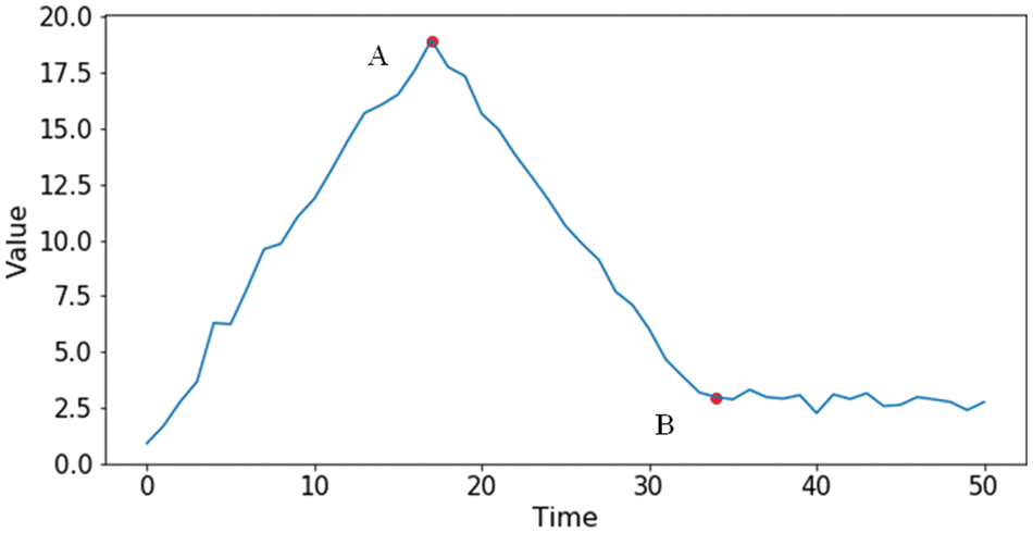
Figure 1: Example of edge points and segmenting

In the context of a time series, an event refers to a significant incident that manifests itself as a pattern within the time series data. For example, a traffic block can be identified as an event, which is depicted as a subsequence within a time series representing bus speeds. This study establishes a correlation between events and the occurrence of frequent patterns within a time series. The higher the frequency of a pattern appearing in a time series, the greater the probability of it being classified as an event. The subsequent definition outlines the characteristics of an event.

Definition 3. Event: Given a time series T = (t1,…, tn), a pattern p is defined as an event e if the proportion of occurrences of p, denoted as support (p), is greater than or equal to the threshold minFreq, that is support (p) ≥ minFreq.

In an event set E, as the length of these events is not fixed, the events that have inclusively or partially overlapping relationships with each other are called multi-granularity events.

Definition 4. Multi-Granularity Event: Given an event set E, for any two events e1 = (t1,…, tm) and e2 = (t1´,…, tn´), there are three possible relationships between them: 1) for any ti in e1 and tj´ in e2, ti ≠ tj´; 2) there are subsequences (ti,…, ti+l) in e1 and subsequences (tj´,…, tj+l´) in e2, (ti,…, ti+l) = (tj´,…, tj+l´); and in 3) there is a subsequence (t1´,…, tm´) in e2, m < n, (t1,…, tm) = (t1´,…, tm´), and the events in set E are called multi-granularity events.

Given a time series T = (t1,…, tn) and a multi-granularity event set E, the problem we are interested in is to match a real-time time series with the set E, to align an unequal real-time series with all the matched events in E and to predict a real-time time series using the aligned events.

4  MGE-SP Framework

To solve the problem, a systematic approach involving several steps is necessary. These steps include detecting, matching, aligning multi-granularity events, and predicting time series data. To facilitate this data analysis process, a methodological system, the Multi-granularity Events Short-Term Prediction (MGE-SP) framework, is proposed, as shown in Fig. 2. The framework consists of three main phases of data processing: multi-granularity event detection, matching, and alignment. Following these processes, a prediction model based on XGBoost is constructed.

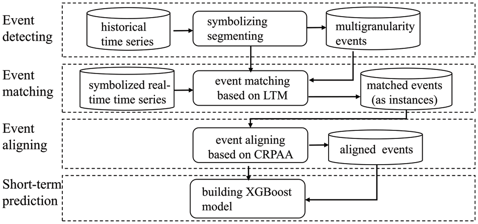
Figure 2: The MGE-SP framework

In the phase of event detection, segmenting a time series is the first step. By symbolizing time series and a self-adaptive segmenting algorithm, a historical time series is partitioned into multi-granularity events. The multi-granularity event detection method based on self-adaptive segmenting [6], SSED, is the previous work.

In the phase of event matching, a real-time time series, which is symbolized, will be matched with the events in the multi-granularity event database. The method of event matching is different depending on different requirements. In this paper, an LTF (Latest Time First) strategy is proposed to match multi-granularity events.

In the phase of event aligning, event instances with different time scales are aligned to an equal length, so that they can be used as a state vector to construct a machine learning-based prediction model. A CRPAA (compression-ratio-based piecewise aggregate approximation) method is proposed to align the multi-granularity events. Of course, other aligning methods can also be employed in this phase if there is a special requirement to be met.

In the phase of time series short-term predicting, an XGBoost-based prediction model is constructed. The aligned event instances as state vectors are used to construct the short-term prediction model of the time series.

5  MGE-SP Method

5.1 Event Matching Based on the Latest Time First

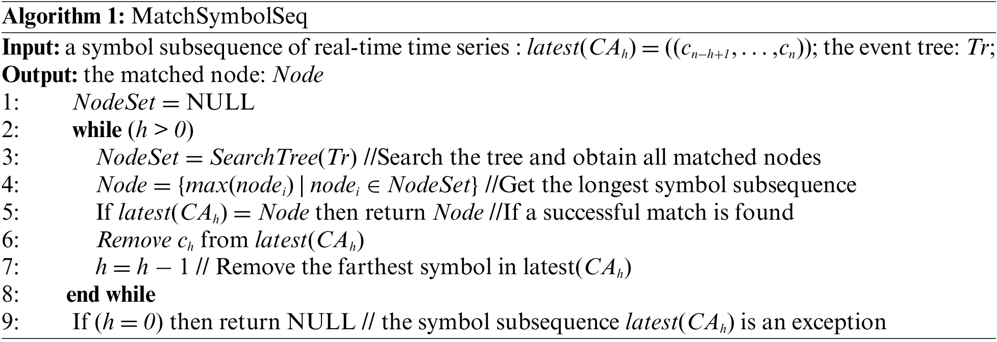
For most prediction methods based on machine learning, selecting the state vector is one of the important factors that determine the performance of the prediction model. In most of the traditional methods, the sliding window is used to segment a time series, and the similarity distance between the segmentations is calculated to match the time series pattern. The prediction model is constructed according to the time series patterns. However, if the source time series patterns are all truncated to equal length, the event matching must result in a worse effect, and finally, the model is unable to be fit effectively. To solve this problem, a method of multi-granularity event matching based on the LTF (Latest Time First) strategy is proposed. The main idea of the strategy is as follows.

Given a symbolic representation of a real-time time series CA = (c1,…, cn), set latest(CAh) = (cn-h+1,…, cn) the latest subsequence of CA, where h is the length of the subsequence. Given an event tree Tr with a height of h and the latest subsequence latest(CAh) with length h, starting at the root node, the nearest subsequence latest(CAh) is matched layer by layer. If there is a node Ni,j in Tr that meets Ni,j.sequence = latest(CAh), a matched event is found, and Ni,j.sequence is a symbolic representation of the matched event, where i denotes the depth of the node and j the node number of the suffix tree. The longest subsequence is chosen. If node Ni,j cannot be matched, the symbol farthest from the current time in latest(CAh) is removed. A new subsequence latest(CAh−1) is constructed. The process is repeated until successful matching is achieved. If the event tree Tr fails to match latest(CA1), the nearest symbol in the CA is considered to be an exception symbol and is removed. The symbolic sequence CA is matched again.

An event tree is created as a suffix tree, in which the root node only serves to index the child nodes. A non-root node Ni,j stores two kinds of information: a subsequence, denoted Ni,j.sequence, whose frequency is greater than minFreq, and the set of starting positions of the subsequence, denoted Ni,j.startindex, in the symbol sequence. More details of the event tree can be found in previous work [6].

To match a symbol sequence CA using the event tree Tr with a height h, four steps should be followed.

Step 1: Match the subsequence latest(CAh) by searching the tree Tr from the root to the leaf nodes; if a successful match is found, go to step 4;

Step 2: Remove the farthest symbol in the latest(CAh) from the current time, i.e., h = h−1; if the length of latest(CAh) is not zero, a new subsequence latest(CAh) is constructed, and return to step 1;

Step 3: Determine that the symbol subsequence latest(CAh) is an exception if there is no successful match to be found in latest(CAh). Remove it from CA, and return;

Step 4: Output the matched node. To match a new symbol subsequence, return to step 1.

The pseudocode of the matching symbol sequence is shown in Algorithm 1.

To ensure the timeliness of matching events, an event rematch is required following new time series data. If the last node that has already matched is Ni,j, suppose that the symbolized representation of the new data is (ck+1,…, ck+m), and a new match of subsequence (ck+1,…, ck+m) starts. The root node of the event tree is Ni,j. If (ck+1,…, ck+m) can successfully be matched at some node in the event tree, the node is the solution. For example, given a symbol sequence CA = (a, b, c, a, c, c, a, b, c, c), as shown in Fig. 3, the matching process of the nearest subsequence (c, c) is as follows. The first step is to match each of the nodes, N1,1, N1,2, and N1,3 using symbol c. As node N1,3 stores a subsequence of c, N1,3 is selected. The second step is to match each of the child nodes, N2,6 and N2,7 of node N1,3 using the first two symbols of the subsequence (c, c), i.e., symbol c, c. As node N2,7 stores the subsequence (c, c), the nearest subsequence (c, c) is successfully matched with node N2,7.

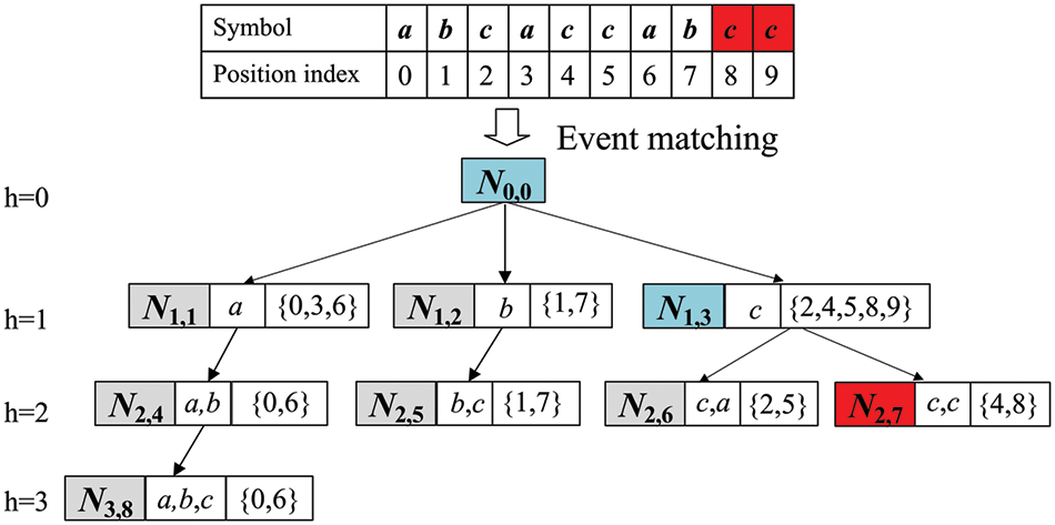
Figure 3: Event matching based on LTF

5.2 Compression Ratio-Based Piecewise Aggregate Approximation

The process of matching a real-time time series using the LTF strategy can obtain all event instances in historical multi-granularity events. However, the duration of event instances may not be the same. For example, all event instances of an event discovered from the dataset, ToeSegmentation1 (http://timeseriesclassification.com/description.php?Dataset=ToeSegmentation1), are shown in Fig. 4. The time scales of these event instances are between 166 and 221, which is not strictly equal and cannot be directly used as a state vector to construct a machine learning-based prediction model. Therefore, dimension alignment is also required on the event instances after matching and obtaining the event instances.

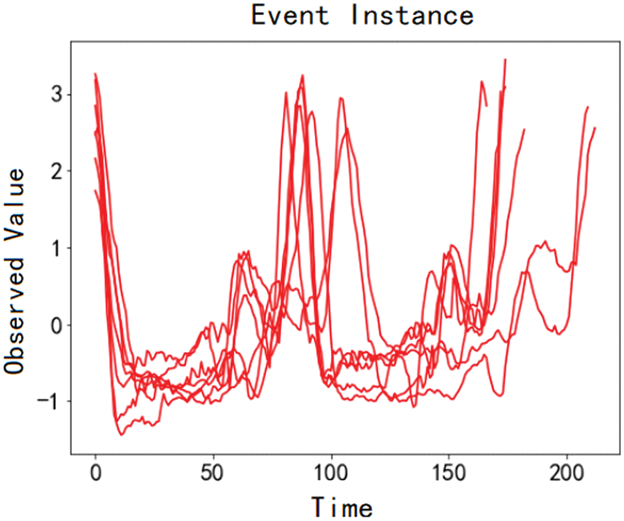
Figure 4: Unequal length event instances

To serve this purpose, an event-aligning method CRPAA (compression-ratio-based piecewise aggregate approximation) is proposed. For a given set of event instances, CRPAA divides all event instances into an equal number of segmentations. Then, each segmentation is approximated by its mean value so that every event instance is mapped into the same low-dimensional space.

Many PLR (piecewise linear representation) methods [29] have been proposed successively to compress time series and eliminate noise in time series. One important goal of PLR is to reduce the dimension of a time series. PAA [30] is a PLR method to uses all the data of the time series for the mean calculation. It is proved that a distance measure between two symbolic strings lower bounds the true distance between the original time series is non-trivial. PAA reduces dimensions by specifying a time window of length w and sliding it over the time series so that the time series can be divided into several equal-length segmentations. Then, each segmentation is approximately represented by the mean of the segmentations. Given a time series T = (t1,…, tn) and a piecewise linear function function (), the time series T can be represented as shown in Eq. (1).

TPLR={function(tep1,tep2)⋯function(tepi,tepi+1)⋯function(tepn−1,tn)(1)

where epi is the ith piecewise point in time series T and function(tepi,tepi+1) is the linear function connecting the piecewise points tepi and tepi+1

Fig. 5 shows the result of using PAA to reduce the dimension of a time series of length 120, where the sliding window length w = 10.

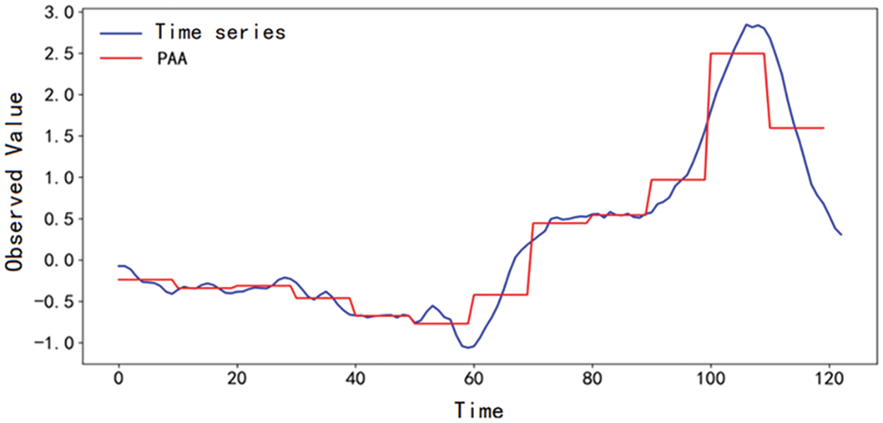
Figure 5: An example of PAA

The compression ratio is often used to evaluate the performance of PLR algorithms. The compression ratio refers to the ratio of the sequence length before and after compression. Given a time series T = (t1,…, tn), if a new sequence of length m can be obtained by using a PLR algorithm, the compression ratio of the PLR algorithm is calculated by Eq. (2).

Compression_ratio=(1−m/n)∗100%(2)

The higher the compression ratio is, the lower the length of the sequence compressed by the PLR algorithm, and the better the compression effect. Given a time series T = (t1,…, tn) and a time window of length w, T can be reduced to n/w dimensions by PAA and approximated as T¯=(t1¯,t2¯,…,tn/w¯). The corresponding relationship between tj¯ and ti is calculated by Eq. (3).

ti¯=(1/w)∑j=w∗(i−1)+1w∗itj(3)

The sequence obtained by using PAA to compress the original sequence can provide a tight lower bound distance measurement, which can effectively control the error with the original time series and provide a better representation effect [30]. Based on PAA, CRPAA divides time series into an equal number of segmentations by specifying the compression ratio to realize dimension alignment of events.

Suppose that latest(CAh) is the symbolic representation of the latest subsequence in a real-time time series, where h is the length of the subsequence, and there are n event instances that are successfully matched and denoted as e1, e2,…, en. For any event instance ei with a length of ni, ei is denoted as (ti,1,ti,2,…,ti,ni), where ei,j is the jth observation value of the ith event instance. For a specified compression ratio cr, the segmenting number of latest(CAh) can be calculated by Eq. (2) as d = h * (1 − cr). Taking d as the fixed segmenting number, ei is divided into a new approximation of the segmentation sequence Wi=(wi,1,wi,2,…,wi,d). In each segmentation sequence wi,j, there is at least one symbol corresponding to an event instance ei. Finally, event instance set {e1, e2, …, en} can be approximated as segmentation sequences {w1¯,w2¯,…,wn¯} where wi¯=(wi,1¯,wi,2¯,…,wi,d¯).

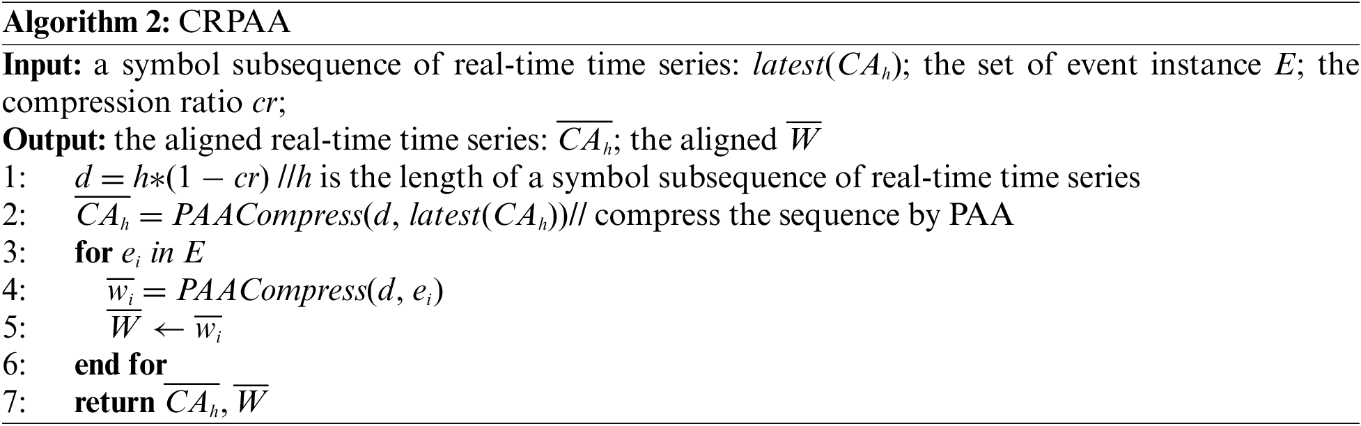
The pseudocode of CRPAA is shown in Algorithm 2.

The performance of CRPAA depends on the compression ratio. The lower the compression ratio is, the more information is retained. However, in this situation, there is the problem of dimensional disaster, although the original time series can be better characterized. In contrast, using a higher compression ratio causes the loss of more information and a lower performance of model fitting, although the dimensional disaster can be avoided and the model fitting process is fast. Therefore, the key to improving CRPAA performance is finding the balance point between maximizing dimensionality reduction and retaining trend information. In time series analysis, a fitting error [31] is usually used to measure the completeness of time series information. A fitting error refers to the degree of fitting between the sequence of dimensionality reduction and the original time series. The lower the fitting error is, the more complete the retained trend information is; otherwise, more information is lost.

Given a time series T = (t1,…, tn), using CRPAA, T is divided into d parts and transformed into a new subsequence W¯=(w1¯,w2¯,…,wd¯) with a length of d. The fitting error fitting_err of W¯ is calculated by Eq. (4).

fitting_err=∑i=1n(ti−W¯⌈(i∗d)/n⌉)2(4)

For a set of event instances {e1, e2, …, en}, using CRPAA, if all the event instances are compressed, the cumulative fitting error is calculated by Eq. (5).

acc_fitting_err=∑i=1nfitting_err(ei)(5)

For example, CRPAA is used to compress the event instances obtained from the dataset ToeSegmentation1, as shown in Fig. 4. Fig. 6 shows the cumulative fitting errors under different compression ratios. When the compression ratio increases from 50% to 70%, the cumulative fitting error changes gently. When the compression rate increases to 75%, the cumulative fitting error has a substantial upward trend. Therefore, by choosing 70% as the recommended compression ratio, the time series can be compressed to the greatest extent while ensuring a low cumulative fitting error.

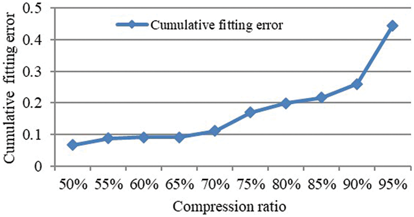
Figure 6: Cumulative fitting errors under different compression ratios

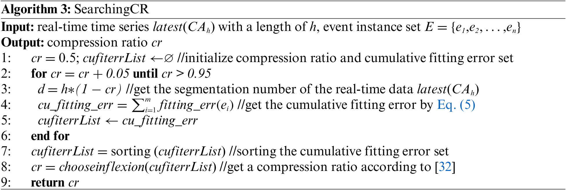
Based on the analysis, a compression ratio search algorithm is proposed. The cumulative fitting error is calculated iteratively by setting an initial compression ratio of 50%, rising by increments of 5% each time to 95%. All the cumulative fitting errors are sorted into a sequence. While searching the sequence using the method in [32], the inflexion point is resolved as the recommended compression ratio. The pseudocode of the compression ratio search algorithm is shown in Algorithm 3.

5.3 XGBoost-Based Prediction Model

Based on the process of dimension alignment, XGBoost is used to construct the short-term prediction model of the time series. XGBoost is a boosting model based on a decision tree, which has advantages, such as fast training speed and a good fitting effect [33]. It performs iterative calculations by constructing multiple weak classifiers and finally uses the cumulative output of multiple weak classifiers as the final prediction result. XGBoost combines the loss function and the regularisation term to construct the objective function, uses the second-order Taylor expansion to enhance the decline rate of the objective function, and reduces the complexity of the model. At the same time, XGBoost supports parallel operation at the feature granularity level, so it has a faster fitting speed than traditional boosting methods, such as gradient boosting trees.

For a given dataset with n examples and m features D={(Xi,Yi)}(|D|=n,Xi∈Rm,Yi∈R, where each Xi corresponds to a real-valued label Yi, the prediction model of XGBoost consisting of K weak classifiers is represented by Eq. (6).

Y~i=∑k=1Kfk(Xi)(6)

where fk(Xi) is the predicted value of the kth tree.

The objective function of XGBoost is constructed by a loss function plus a penalty function of the regularisation term, as shown in Eq. (7).

J=∑i=1nloss(Yi,Y~i)+∑k=1KΩ(fk)(7)

where loss(Yi,Yi~) is the deviation function between the target Yi and the prediction value Y~i. Ω(fk) is the penalty function of the model, as shown in Eq. (8).

Ω(fk)=γ|T|+12λ∑j=1Tωj2(8)

where γ and λ are the penalty weights and |T| is the number of leaf nodes in the kth decision tree. ωj is the weight of the jth leaf node in this decision tree.

XGBoost is essentially an integration that uses the residual to construct multiple weak classifiers that work together to make the final decision. Therefore, the objective function can be further represented as follows in Eq. (9).

J(fk)=∑i=1nloss(Yi,Y~i(k−1)+fk(Xi))+Ω(fk)+C(9)

where Y~i(k−1) is the cumulative predicted value obtained from the first k − 1 trees, and C is the prescribed constant term.

To construct the short-term prediction model of the time series, the aligned event instances as state vectors are used to train the model. The training framework for the short-term prediction model is shown in Fig. 7.

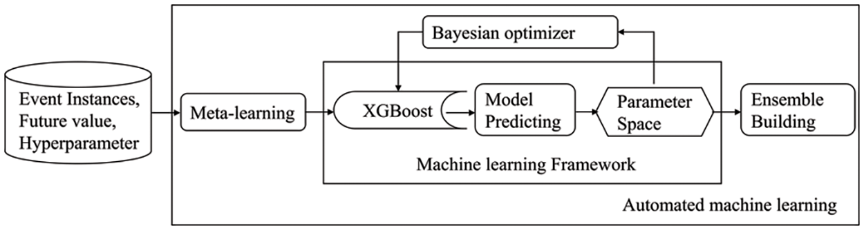
Figure 7: Automated training framework for XGBoost models

The Bayesian optimizer constructs a posterior model based on the performance of the available samples in the optimization objective function. In each iteration, depending on the previous observed historical performance, the next optimization is performed, continuously updating the posterior probability model to search for the local optimal parameters in the optimization objective function. As the entire machine learning framework has a large parameter space, Bayesian optimization is slow to start. A meta-learning approach is used for Bayesian optimization. Based on meta-learning, many configurations are selected, and their results are used to seed Bayesian optimization. The whole machine-learning process is highly automated and can save users much time.

The automated training framework based on the Bayesian optimizer is used to optimize the parameters of XGBoost. There are three steps altogether:

1. Align the event instances with which a real-time series time is successfully matched together with the future observations corresponding to the event instances using CRPAA. Then, the event instances are input into the training framework as true values.

2. Initialise the Bayesian optimizer using meta-learning.

3. Predict future observations using the parameters of the current model to evaluate the difference between the true value and the predicted value and to optimize the parameters using the Bayesian optimizer according to the difference.

6  Performance Evaluation

To evaluate the performance of the MGE-SP, we took two experiments, a customized passenger transport in Xiamen, China, and a stock to analyze our method. Moreover, for a quantitative analysis, two methods, the ARIMA method [8] and the k-means-SVR method [7], are chosen for comparison.

6.1 Experiment on Customized Passenger Transport

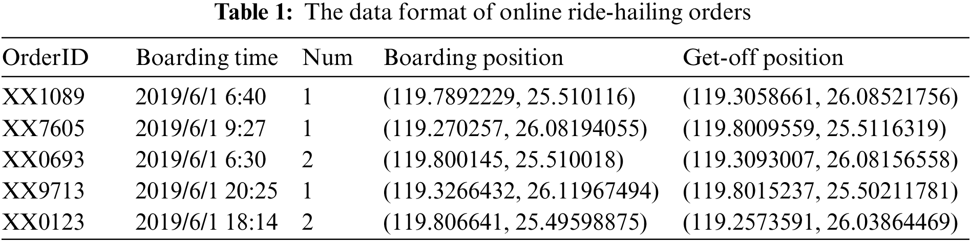
The dataset is collected from an online ride-hailing service company in Xiamen, China. We extracted some of the orders from June to December 2019 (https://pan.hqu.edu.cn/share/f6a8e453a9e31af1803c6a38d4). In the dataset, there is some basic information, such as passenger numbers, boarding times, and positions, in each order, as shown in Table 1. To obtain the time series of passenger flow, the dataset should be preprocessed. The real value ti in a time series T = (t1,…, tn) is a statistic on the number of passengers on board at different periods. The period is usually half an hour.

To make a better experimental comparison, the time series of passenger flow is further divided into two parts. In this experiment, the data are used as the training set except for the data from the last 5 days (December 27, 2019 to December 31, 2019). The data of the last 5 days are used as the testing set, which is selected to be compared with the prediction results, as shown in Fig. 8.

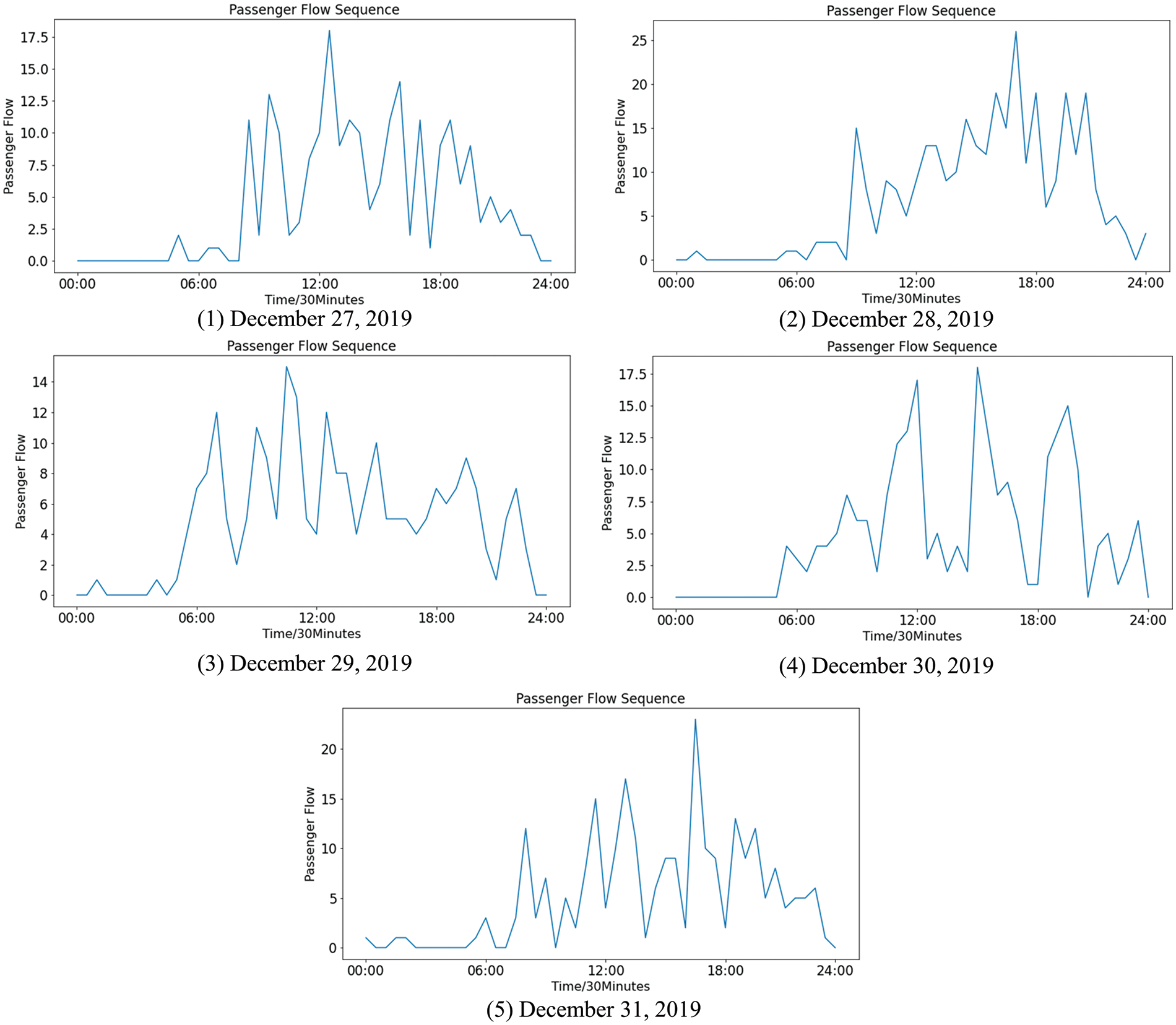
Figure 8: The sequence of actual passenger flow

The experiment has three steps: 1) the time series in the last five days are matched with the multi-granularity events using the LTF strategy; 2) the real-time data and the event instances are aligned using CRPAA; and 3) the XGBoost model for short-term prediction is constructed, during which the dimension-aligned event instances are used as the state vectors.

Before the three steps, the multi-granularity events should be resolved using the SSED method, which was proposed in [6]. In this experiment, the parameters used in SSED are the adjacency segmentation length m, minimum segmenting granularity r, and BIRCH clustering distance threshold δ. Setting the parameters m = 2, d = 4, r = 30 min, and δ = 1.3, SSED finds 1339 events in the historical dataset. Due to space limitations, only two events solved using the algorithm SSED are shown on the right of Fig. 9, and their instances are shown on the left of Fig. 9.

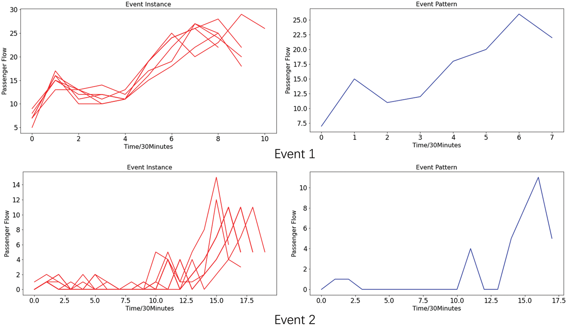
Figure 9: The example of two events

Step 1) The time series in the last five days are matched with the multi-granularity events using the LTF strategy.

After symbolizing the data of the prediction day, the real-time sequence of 30 min is matched with the event instances based on the LTF strategy. To better simulate the real situation, the event matching is restarted every 30 min.

Step 2) The real-time data and the event instances are aligned using CRPAA.

After extracting the event instances with which the real-time sequence is successfully matched, the CRPAA algorithm is used to align the dimensions of the event instances. As the main parameter of CRPAA is the compression ratio, Algorithm 3 is used to search for the optimal solution for the compression ratio.

Step 3) The XGBoost model for short-term prediction is constructed, during which the dimension-aligned event instances are used as the state vectors.

The event instances processed in step 2 are used as the state vector to construct the short-term prediction model based on XGBoost. In this paper, the grid search algorithm is used to automatically optimize the parameters involved in XGBoost [34]. Based on the XGBoost model with optimized parameters, the difference between the predicted values and the true values of the passenger flow is shown in Fig. 10.

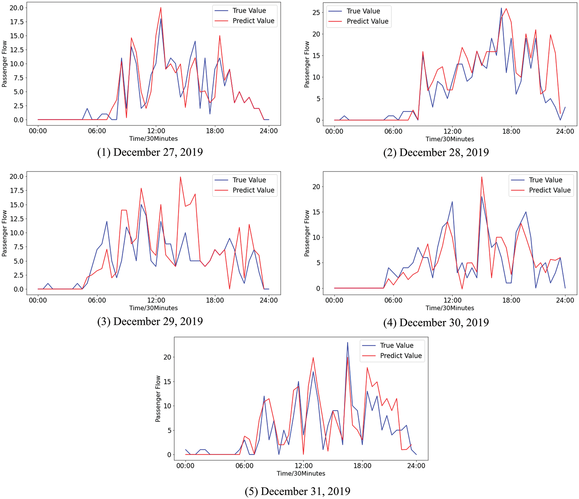
Figure 10: The difference between the predicted values and the true values of the passenger flow using MGE-SP

For quantitative analysis, two methods, the ARIMA method proposed in [8] and the k-means-SVR method proposed in [7], are chosen for comparison. The experimental data remain the same. The prediction results of ARIMA and k-means-SVR are shown in Figs. 11 and 12, respectively.

Figure 11: The difference between the predicted values and the true values of the passenger flow by ARIMA

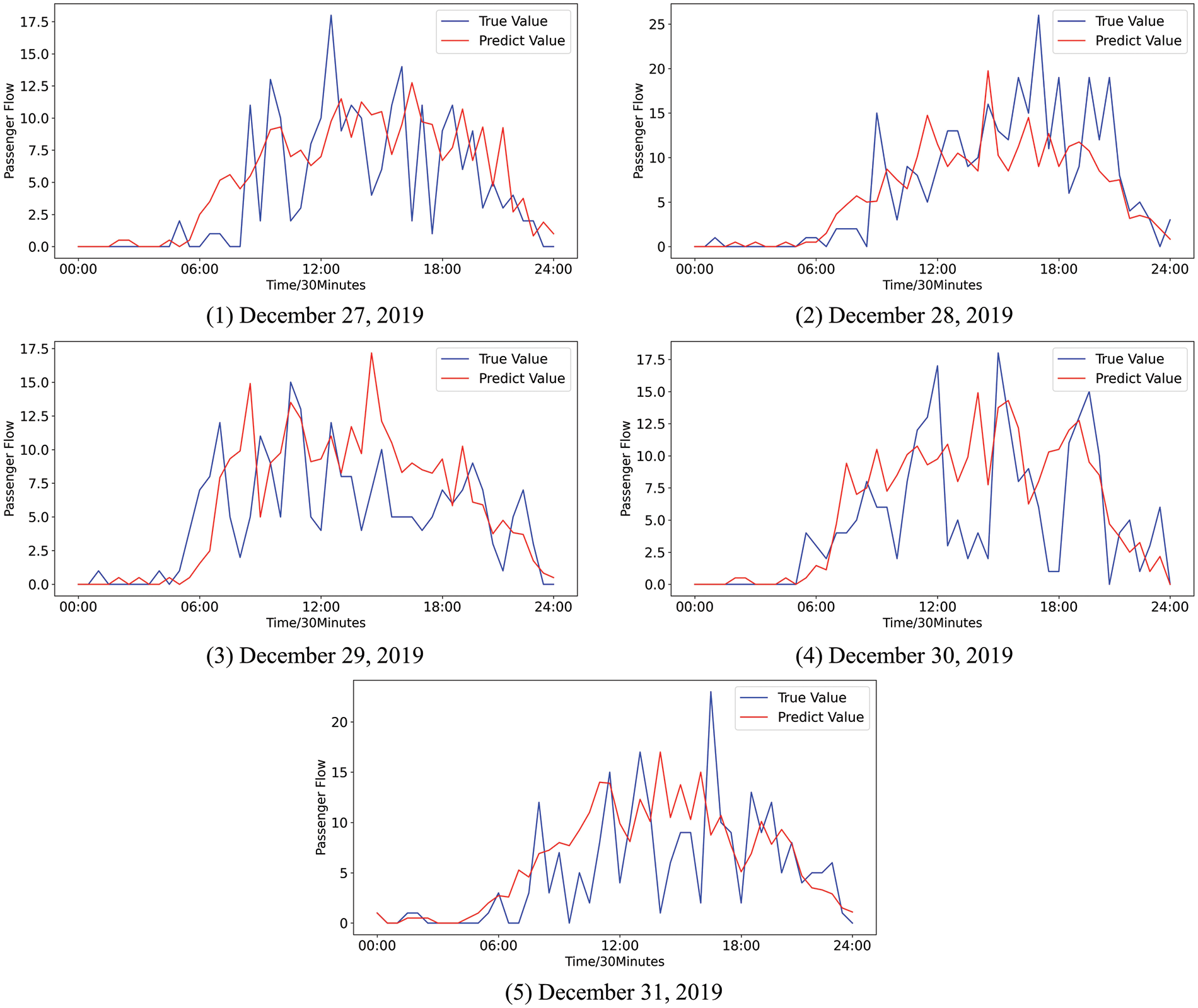
Figure 12: The difference between the predicted values and the true values of the passenger flow by k-means-SVR

Fig. 10 shows that the trend and volatility of the passenger flow can be effectively fitted by MGE-SP. In Fig. 11, ARIMA predicts the overall trend of passenger flow to some extent but cannot effectively fit the fluctuation of passenger flow. This is because the passenger flow is a complex nonlinear system that is affected by weather, holidays, seasons, and other factors. As a linear model, ARIMA has difficulty effectively fitting the passenger flow time series with nonlinear and nonstationary characteristics and cannot accurately track the fluctuation of passenger flow in real time. In Fig. 12, as a nonlinear prediction model, k-means-SVR has a higher tendency to track the passenger flow series in peak hours and has a better fitting effect on the fluctuation of the passenger flow than ARIMA. However, in terms of overall trends, the fitting effect is weaker than that of ARIMA and MGE-SP.

In this paper, MAE (mean absolute error) and RMSE (root mean square error) are used to evaluate the prediction effect, as shown in Eqs. (10) and (11).

MAE=1s∑i=1s|Yi−Y~i|(10)

RMSE=1s∑i=1s(Yi−Y~i)2(11)

where Yi represents the actual value at time i, Y~i represents the predicted value at time i, and s is the maximum step size of the short-time prediction in this iteration.

Fundamentally, MAE and RMSE measure the same item: the average distance of the error between the true value and the predicted value. The lower the MAE and RMSE values are, the better the model’s prediction. The comparison of the MAE and RMSE of the three methods is shown in Table 2. ARIMA achieved the highest error values on December 27 and December 30 because ARIMA is good at fitting stable sequences instead of high variance sequences, such as passenger flow. ARIMA has difficulty effectively capturing its trend, resulting in a large deviation between the predicted value and the real value.

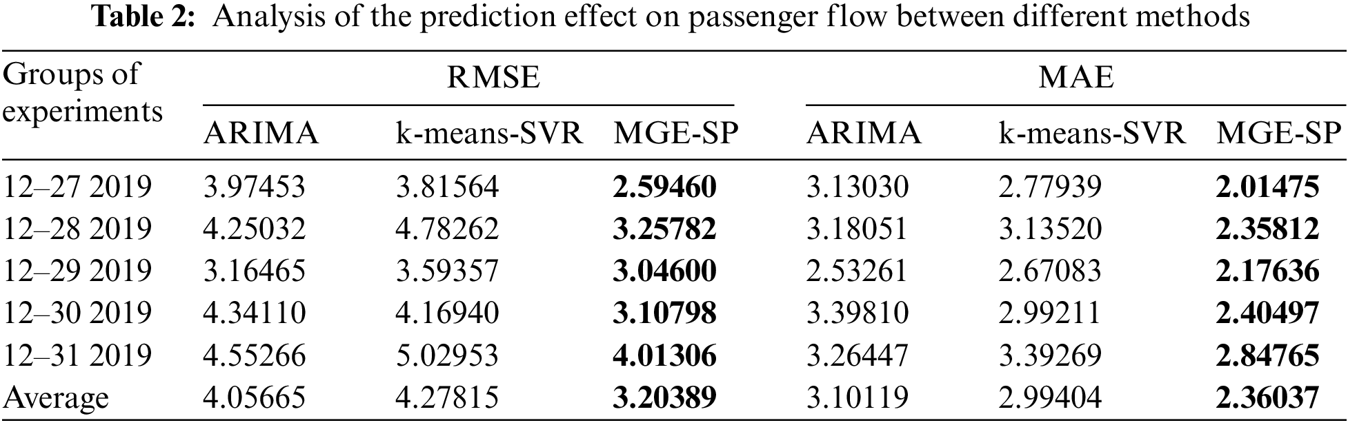
K-means-SVR achieved the maximum error on December 28, December 29, and December 31. K-means-SVR matched the pattern by the sliding window and clustering. However, there were multiple granularity events in the passenger flow sequence. It is difficult to accurately identify the start time point and duration of multi-granularity events through a fixed time window, which is used by most pattern recognition methods. It causes the wrong judgment for patterns and makes the predicted value deviate too much from the true value.

MGE-SP has achieved the lowest error in the last five days. Compared with the other two models, MGE-SP tracks the trend of passenger flow more accurately, fits the true value better, and obtains the predicted value with the lowest deviation from the true value. MGE-SP matches events through the state vector represented by the symbol sequence of real-time data. The method breaks through the limitations of traditional methods that can only match events with fixed lengths.

6.2 Experiment on Stock

The stock dataset is collected from the big data platform, Tushare (https://tushare.pro/). The closing prices of four stocks, Ping An Bank, Vanke, ZTE, and OCT, on working days are selected from the platform as the experimental dataset. The time range of the four datasets is from June 04, 2010, to June 17, 2020, for a total of 2,486 days.

The closing prices of the four stocks over the selected time frame are shown in Fig. 13. In this paper, the period from May 17, 2020, to June 17, 2020, is used as the testing set, and the rest of the historical data are used as the training set. MAE and RMSE are used to measure the error between the predicted value and the true value.

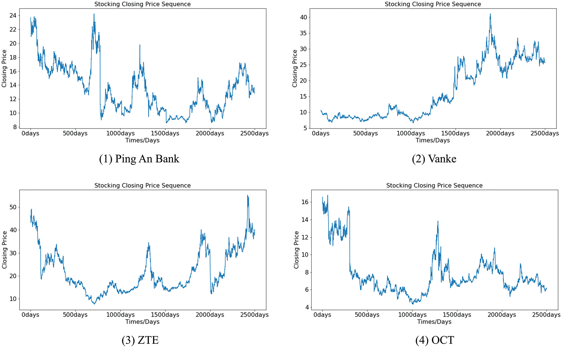
Figure 13: The closing price of stocks

The differences between the predicted value and the true value of the stock closing price by MGE-SP, ARIMA, and k-means-SVR are shown in Figs. 14–16, respectively. It can be seen from Fig. 14 that MGE-SP makes an effective fit to the trend and amplitude of variation. As a linear model, ARIMA can fit stable sequences well, such as OCT. However, it is still difficult to fit high-variance sequences that have obvious fluctuations in the short term, such as ZTE. Similarly, k-means-SVR is more sensitive to short-term stock fluctuations, while it is not as stable and accurate as ARIMA in tracking trends.

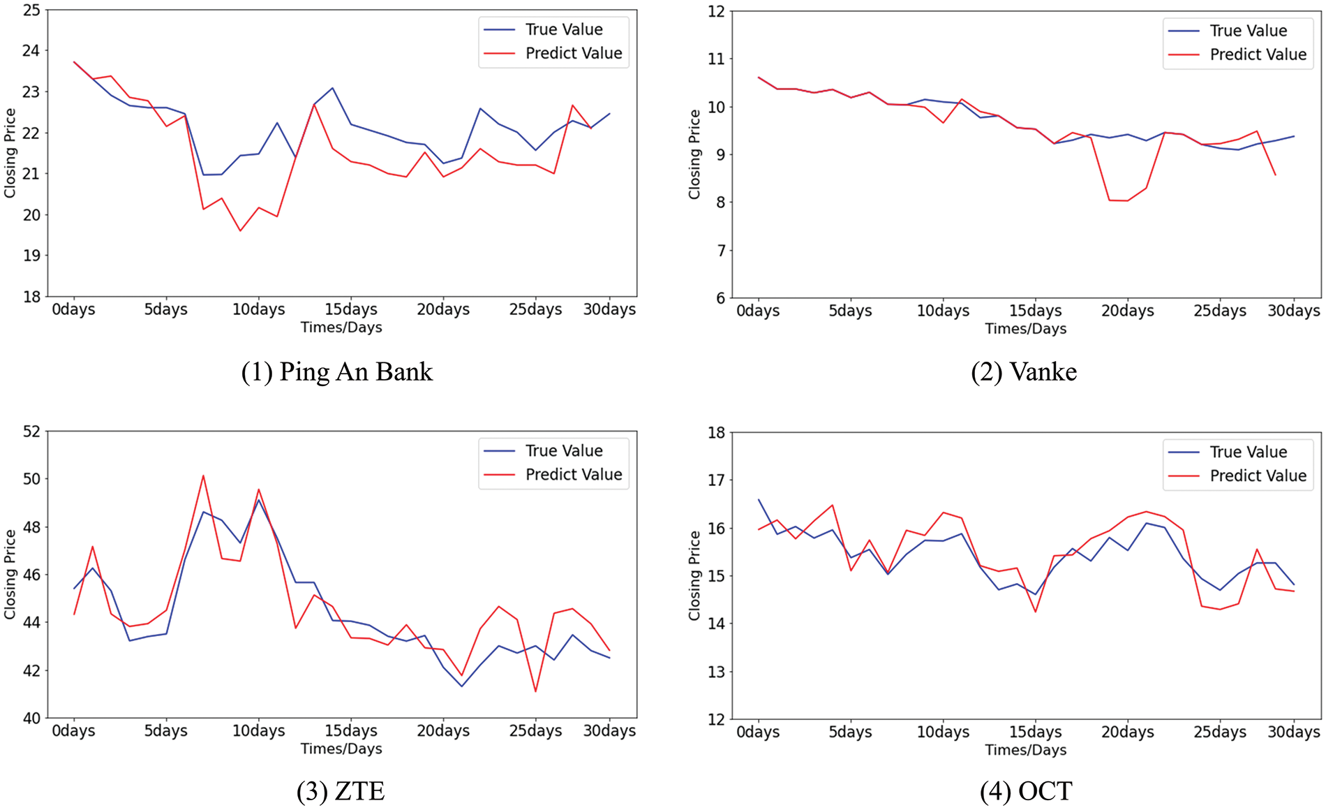
Figure 14: The difference between the predicted values and the true values of stocks using MGE-SP

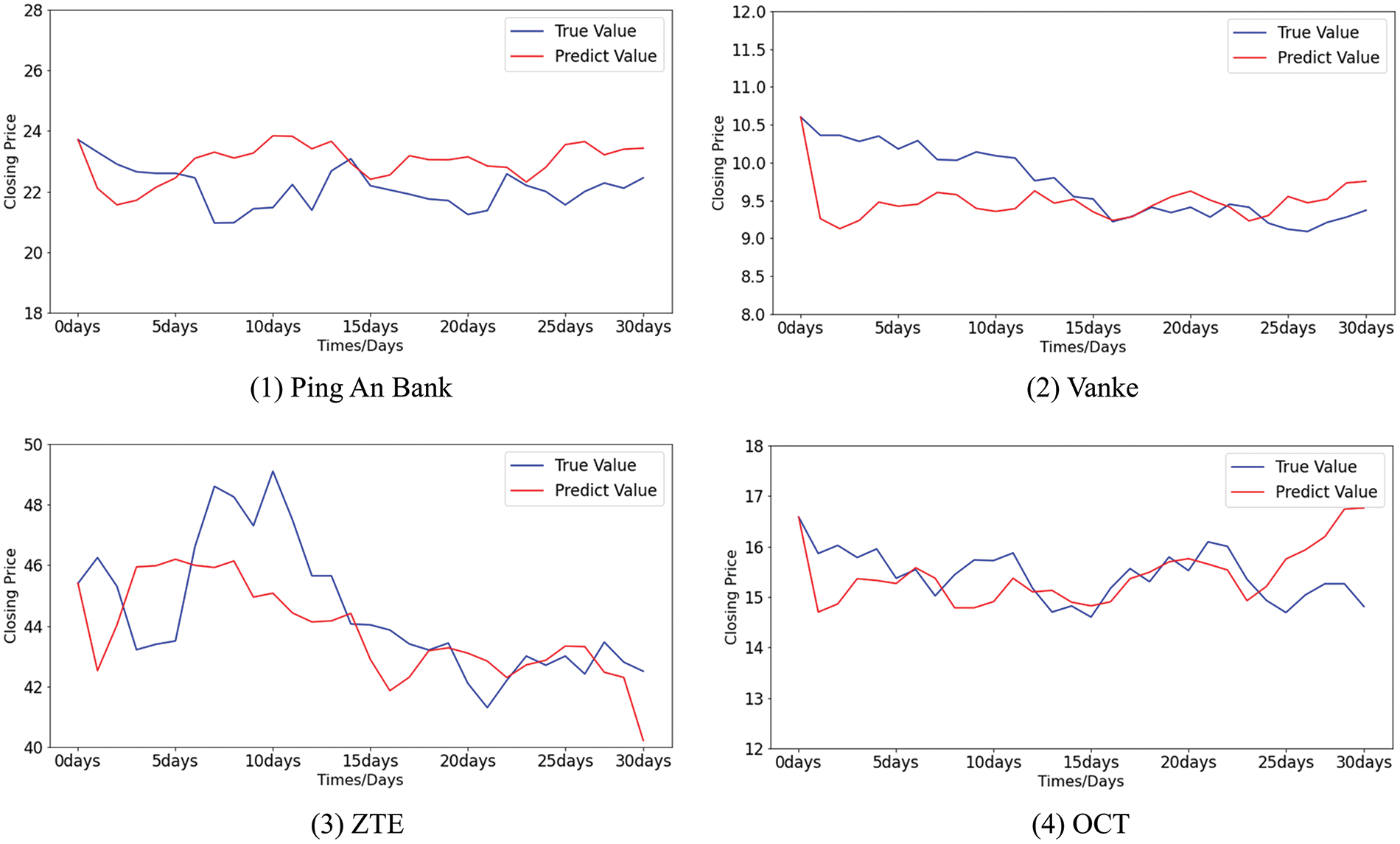
Figure 15: The difference between the predicted values and the true values of stocks using ARIMA

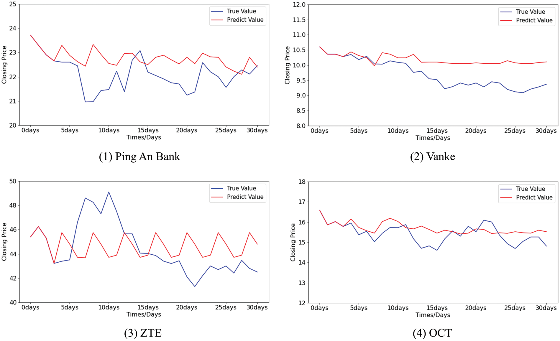
Figure 16: The difference between the predicted values and the true values of stocks using k-means-SVR

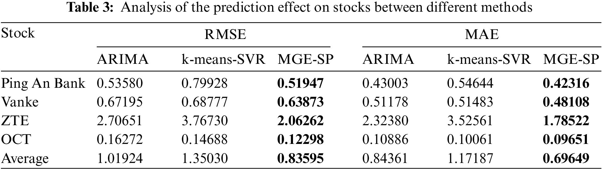
Table 3 shows the MAE and RMSE comparison between the predicted values and the true values of the three methods. MGE-SP achieves the lowest MAE and RMSE in the testing set of four stocks. Experimental results show that MGE-SP can more effectively fit stock data and is superior to ARIMA and k-means-SVR in tracking trend and volatility analysis of the stock data. MGE-SP has good robustness.

7  Conclusion

In our research, we have focused on the analysis of multi-granularity event matching and alignment methods in the computer domain. We have integrated these methods with previously studied multi-granularity event segmentation techniques to create a comprehensive system named MGE-SP. This system facilitates the preprocessing of time series data and significantly improves the accuracy of short-term predictions. Our primary objective is to leverage MGE-SP to enhance the precision of our forecasting models.

We evaluated the results of MGE-SP with two indicators, RMSE and MAE. Through experimentation, MGE-SP demonstrates efficiency by achieving lower average RMSE and MAE scores, 3.204 and 2.360 for the first experiment and 0.836 and 0.696 for the second experiment, compared to other methods. This has led to an overall performance boost. The results reveal that the MGE-SP methodology outperforms traditional methods, supported by the data selected from different domains, reinforcing the universality of MGE-SP.

Our research contributes novel ideas and approaches to the domain of multi-granularity event matching and alignment. Specifically, we have developed the LTF strategy and algorithm, which effectively decreases matching errors arising from equal-length time series patterns. Additionally, we employ the piecewise aggregate approximation method, which leverages compression ratio to align the time scales of multi-granularity events. These aligned events can serve as state vectors for machine learning-based prediction methodologies.

Although MGE-SP can effectively reduce the prediction error of time series, the matching of large-scale multi-granularity events comes at the cost of sacrificing matching efficiency. Therefore, future work will focus on enhancing the efficiency of matching multi-granularity events. This may involve considering events as high-order features or exploring the potential of incorporating both high-order and low-order features in the matching process.

Acknowledgement: Thanks to Jiang Peizhou from the Xiamen GNSS Development & Application Co., Ltd. He provided the necessary scientific data for the work. Thanks to Dr. Mengxia Liang from Harbin Institute of Technology, who provided many valuable suggestions for the revision of this article.

Funding Statement: This research was funded by the Fujian Province Science and Technology Plan, China (Grant Number 2019H0017).

Author Contributions: The authors confirm contribution to the paper as follows: study conception and design: Haibo Li; data collection: Haibo Li; analysis and interpretation of results: Yongbo Yu, Zhenbo Zhao and Xiaokang Tang; draft manuscript preparation: Haibo Li, Yongbo Yu. All authors reviewed the results and approved the final version of the manuscript.

Availability of Data and Materials: The data comes from publicly available datasets on Tushare (https://tushare.pro/), including the closing prices of stocks, and from an online ride-hailing service company (https://pan.hqu.edu.cn/share/f6a8e453a9e31af1803c6a38d4).

Conflicts of Interest: The authors declare that they have no conflicts of interest to report regarding the present study.

References

1. M. Liang, X. Wang and S. Wu, “A novel time-sensitive composite similarity model for multivariate time-series correlation analysis,” Entropy, vol. 23, no. 6, pp. 731, 2021. [Google Scholar] [PubMed]

2. M. Liang, S. Wu, X. Wang and Q. Chen, “A stock time series forecasting approach incorporating candlestick patterns and sequence similarity,” Expert Systems with Applications, vol. 205, pp. 117595, 2022. [Google Scholar]

3. P. Pelka, “Analysis and forecasting of monthly electricity demand time series using pattern-based statistical methods,” Energies, vol. 16, no. 2, pp. 827, 2023. [Google Scholar]

4. Y. Perez and F. H. Pereira, “Estimating pandemic effects in urban mass transportation systems: An approach based on visibility graphs and network similarity,” Physica A: Statistical Mechanics and its Applications, vol. 620, pp. 128772, 2023. [Google Scholar]

5. D. B. Jia, Z. X. Xu, Y. C. Wang and R. Ma, “Application of intelligent time series prediction method to dew point forecast,” Electronic Research Archive, vol. 31, no. 5, pp. 2878–2899, 2023. [Google Scholar]

6. H. Li and Y. Yu, “Detecting a multi-granularity event in an unequal interval time series based on self-adaptive segmenting,” Intelligent Data Analysis, vol. 25, no. 6, pp. 1407–1429, 2021. [Google Scholar]

7. L. F. S. Vilela, R. C. Leme, C. A. M. Pinheiro and O. A. S. Carpinteiro, “Forecasting financial series using clustering methods and support vector regression,” Artificial Intelligence Review, vol. 52, no. 2, pp. 743–773, 2019. [Google Scholar]

8. C. Kocak, “ARMA(p,q) type high order fuzzy time series forecast method based on fuzzy logic relations,” Applied Soft Computing Journal, vol. 58, pp. 92–103, 2017. [Google Scholar]

9. A. M. Sathe and N. S. Upadhye, “Estimation of the parameters of symmetric stable ARMA and ARMA-GARCH models,” Journal of Applied Statistics, vol. 49, no. 11, pp. 2964–2980, 2022. [Google Scholar] [PubMed]

10. N. H. Hussin, F. Yusof, A. R. Jamaludin and S. M. Norrulashikin, “Forecasting wind speed in peninsular Malaysia: An application of Arima and Arima-Garch models,” Pertanika Journal of Science and Technology, vol. 29, no. 1, pp. 31–58, 2021. [Google Scholar]

11. I. J. Cruz, “The fitting of SARIMA model to tourism in mexican roads,” Periplo Sustentable, no. 41, pp. 431–446, 2021. [Google Scholar]

12. P. B. Kumar and K. Hariharan, “Time series traffic flow prediction with hyper-parameter optimized ARIMA models for intelligent transportation system,” Journal of Scientific and Industrial Research, vol. 81, pp. 408–415, 2022. [Google Scholar]

13. H. H. Huang, N. H. Chan, K. Chen and C. K. Ing, “Consistent order selection for arfima processes,” Annals of Statistics, vol. 50, no. 3, pp. 1297–1319, 2022. [Google Scholar]

14. E. M. de Oliveira and F. L. Cyrino Oliveira, “Forecasting mid-long term electric energy consumption through bagging ARIMA and exponential smoothing methods,” Energy, vol. 144, pp. 776–788, 2018. [Google Scholar]

15. A. W. Adewuyi, “Modelling stock prices with exponential weighted moving average (EWMA),” Journal of Mathematical Finance, vol. 6, no. 1, pp. 99–104, 2016. [Google Scholar]

16. Y. Chang, X. Wang, M. Xue, Y. Liu and F. Jiang, “Improving language translation using the hidden markov model,” Computers, Materials & Continua, vol. 67, no. 3, pp. 3921–3931, 2021. [Google Scholar]

17. E. S. M. El-Kenawy, A. Ibrahim, N. Bailek, K. Bouchouicha, M. A. Hassan et al., “Hybrid ensemble-learning approach for renewable energy resources evaluation in algeria,” Computers, Materials & Continua, vol. 71, no. 2, pp. 5837–5854, 2022. [Google Scholar]

18. F. Guo, Z. Liu, W. Hu and J. Tan, “Gain prediction and compensation for subarray antenna with assembling errors based on improved XGBoost and transfer learning,” IET Microwaves, Antennas and Propagation, vol. 14, no. 6, pp. 551–558, 2020. [Google Scholar]

19. Y. J. Natarajan and D. S. Nachimuthu, “New SVM kernel soft computing models for wind speed prediction in renewable energy applications,” Soft Computing, vol. 24, no. 15, pp. 11441–11458, 2020. [Google Scholar]

20. H. Guo, W. Pedrycz and X. Liu, “Hidden markov models based approaches to long-term prediction for granular time series,” IEEE Transactions on Fuzzy Systems, vol. 26, no. 5, pp. 2807–2817, 2018. [Google Scholar]

21. J. Mei, Y. De Castro, Y. Goude, J. M. Azaïs and G. Hébrail, “Nonnegative matrix factorization with side information for time series recovery and prediction,” IEEE Transactions on Knowledge and Data Engineering, vol. 31, no. 3, pp. 493–506, 2019. [Google Scholar]

22. P. Y. Ting, T. Wada, Y. L. Chiu and M. T. Sun, “Freeway travel time prediction using deep hybrid model-taking sun yat-sen freeway as an example,” IEEE Transactions on Vehicular Technology, vol. 69, no. 8, pp. 8257–8266, 2020. [Google Scholar]

23. Y. Lv, Y. Duan, W. Kang, Z. Li and F. Y. Wang, “Traffic flow prediction with big data: A deep learning approach,” IEEE Transactions on Intelligent Transportation Systems, vol. 16, no. 2, pp. 865–873, 2015. [Google Scholar]

24. S. Siami-Namini, N. Tavakoli and A. Siami Namin, “A comparison of ARIMA and LSTM in forecasting time series,” in Proc. of 17th IEEE Int. Conf. on Machine Learning and Applications, ICMLA 2018, Orlando, FL, USA, pp. 1394–1401, 2019. [Google Scholar]

25. H. Kang, S. Yang, J. Huang and J. Oh, “Time series prediction of wastewater flow rate by bidirectional LSTM deep learning,” International Journal of Control, Automation and Systems, vol. 18, no. 12, pp. 3023–3030, 2020. [Google Scholar]

26. X. Zhang, S. Kuenzel, N. Colombo and C. Watkins, “Hybrid short-term load forecasting method based on empirical wavelet transform and bidirectional long short-term memory neural networks,” Journal of Modern Power Systems and Clean Energy, vol. 10, no. 5, pp. 1216–1228, 2022. [Google Scholar]

27. M. Ehteram, F. Panahi, A. N. Ahmed, Y. F. Huang, P. Kumar et al., “Predicting evaporation with optimized artificial neural network using multi-objective salp swarm algorithm,” Environmental Science and Pollution Research, vol. 29, no. 7, pp. 10675–10701, 2022. [Google Scholar] [PubMed]

28. P. Liu, J. Liu and K. Wu, “CNN-FCM: System modeling promotes stability of deep learning in time series prediction,” Knowledge-Based Systems, vol. 203, pp. 106081, 2020. [Google Scholar]

29. P. Cruz and H. Cruz, “Piecewise linear representation of finance time series: Quantum mechanical tool,” Acta Physica Polonica A, vol. 138, no. 1, pp. 21–24, 2020. [Google Scholar]

30. E. Keogh, K. Chakrabarti, M. Pazzani and S. Mehrotra, “Dimensionality reduction for fast similarity search in large time series databases,” Knowledge and Information Systems, vol. 3, no. 3, pp. 263–286, 2001. [Google Scholar]

31. E. J. Parish and K. T. Carlberg, “Time-series machine-learning error models for approximate solutions to parameterized dynamical systems,” Computer Methods in Applied Mechanics and Engineering, vol. 365, pp. 112990, 2020. [Google Scholar]

32. H. Yin, S. Q. Yang, X. Q. Zhu, S. D. Ma and L. M. Zhang, “Symbolic representation based on trend features for knowledge discovery in long time series,” Frontiers of Information Technology and Electronic Engineering, vol. 16, no. 9, pp. 744–758, 2015. [Google Scholar]

33. T. Chen and C. Guestrin, “XGBoost: A scalable tree boosting system,” in Proc. of the 22nd ACM SIGKDD Int. Conf. on Knowledge Discovery and Data Mining, San Francisco, California, USA, pp. 785–794, 2016. [Google Scholar]

34. A. Ogunleye and Q. G. Wang, “XGBoost model for chronic kidney disease diagnosis,” IEEE/ACM Transactions on Computational Biology and Bioinformatics, vol. 17, no. 6, pp. 2131–2140, 2020. [Google Scholar] [PubMed]