
 Submit a Paper
 Propose a Special lssue
 Open Access
ARTICLE

Selective and Adaptive Incremental Transfer Learning with Multiple Datasets for Machine Fault Diagnosis
1 School of Science and Technology, Hong Kong Metropolitan University, Hong Kong, 999077, China
2 Department of Computer Science and Information Engineering, Asia University, Taichung, 41354, Taiwan
3 Center for Advanced Information Technology, Kyung Hee University, Seoul, 02447, Korea
4 Symbiosis Centre for Information Technology, Symbiosis International University, Pune, Maharashtra, 411042, India
5 Department of Electrical and Computer Engineering, Lebanese American University, Beirut, 1102, Lebanon
6 School of Computing, Skyline University College, Sharjah, 1797, United Arab Emirates
7 Department of Business Administration, Asia University, Taichung, 41354, Taiwan
8 Center for Interdisciplinary Research, University of Petroleum and Energy Studies, Dehradun, 248007, India
9 Department of Computer Science & Engineering, Chandigarh University, Chandigarh, 160036, India
10 Centro de Investigación en Computación, Instituto Politécnico Nacional, UPALM-Zacatenco, Mexico City, 07320, Mexico
* Corresponding Authors: Kwok Tai Chui. Email: ; Brij B. Gupta. Email:
(This article belongs to the Special Issue: Development and Industrial Application of AI Technologies)
Computers, Materials & Continua 2024, 78(1), 1363-1379. https://doi.org/10.32604/cmc.2023.046762
Received 13 October 2023; Accepted 27 November 2023; Issue published 30 January 2024
 View Full Text
 Download PDF
Abstract
The visions of Industry 4.0 and 5.0 have reinforced the industrial environment. They have also made artificial intelligence incorporated as a major facilitator. Diagnosing machine faults has become a solid foundation for automatically recognizing machine failure, and thus timely maintenance can ensure safe operations. Transfer learning is a promising solution that can enhance the machine fault diagnosis model by borrowing pre-trained knowledge from the source model and applying it to the target model, which typically involves two datasets. In response to the availability of multiple datasets, this paper proposes using selective and adaptive incremental transfer learning (SA-ITL), which fuses three algorithms, namely, the hybrid selective algorithm, the transferability enhancement algorithm, and the incremental transfer learning algorithm. It is a selective algorithm that enables selecting and ordering appropriate datasets for transfer learning and selecting useful knowledge to avoid negative transfer. The algorithm also adaptively adjusts the portion of training data to balance the learning rate and training time. The proposed algorithm is evaluated and analyzed using ten benchmark datasets. Compared with other algorithms from existing works, SA-ITL improves the accuracy of all datasets. Ablation studies present the accuracy enhancements of the SA-ITL, including the hybrid selective algorithm (1.22%–3.82%), transferability enhancement algorithm (1.91%–4.15%), and incremental transfer learning algorithm (0.605%–2.68%). These also show the benefits of enhancing the target model with heterogeneous image datasets that widen the range of domain selection between source and target domains.Keywords
Machine fault diagnosis (MFD) using machine learning algorithms gains unprecedented attention due to its ability to detect machine failure and automatically improve industrial maintenance management. This maintenance is categorized as run-time-failure, preventive, and predictive maintenance [1]. Traditionally, machine learning models have been built based on model training with datasets from the desired domain. Due to its ability to enhance the model’s performance and reduce the training time, transfer learning has played an important role in recent MFD research works, which was thoroughly discussed in the review article [2]. The rationales are two-fold: (i) the characteristics of the fault data across different datasets share similarities and dissimilarities where the former can be transferred from a source to target datasets, and (ii) the machine learning model imitates the diagnosticians where knowledge can be shared to diagnose different types of machines. It is worth noting that transfer learning can not only apply to homogeneous datasets but also receives benefits from heterogeneous datasets [3]. It can be seen from the major existing works that the bottleneck in MFD is attributable to the restriction of transfer learning between source-target domain.
This paper proposes a new research initiative that leverages the ability to transfer knowledge transfer from multiple source datasets to single target datasets. The design of the algorithm for MFD should enable the following features: (i) reducing the computational power, (ii) reducing the time complexity, (iii) prioritizing the source datasets to be transferred, (iv) avoiding negative transfer, and (v) moving the solution toward the optimal solution.
The paper is organized in the following manner: The initial section examines and analyzes the methods, results, and limitations of previous research, which leads to the proposal of a novel algorithm that addresses these limitations. The second section outlines the formulation and design of the proposed algorithm’s methodology. The third section provides a summary of ten benchmark datasets, followed by a comparison and evaluation of the proposed algorithm’s performance. The fourth section conducts ablation studies to explore the effectiveness of the proposed algorithm’s components. Lastly, the paper concludes with a summary and discusses potential directions for future research.
Many transfer learning models were formulated using a single source and single target. However, their experience and insights can inspire the design and formulation of our proposed algorithm.
A pre-trained convolutional neural network (CNN) model was employed to fine-tune the target model for bearing fault diagnosis [4]. The performance evaluation was based on nine parameter strategies with seven testing scenarios. The average accuracies ranged from 61.1% to 98.6%. In [5], an adversarial domain-invariant generalization approach was proposed to fuse the knowledge from various datasets. The domain classifier and feature extractor learned the domain-invariant knowledge. The average accuracies were 98% and 93% using the newly collected and existing datasets. Usually, the source datasets may contain multiple subsets known as subdomains. A three-module algorithm adopting multiple adversarial domains was proposed for the fault diagnosis of rolling bearings [6]. The authors of the work [7] transferred the knowledge from multiple subdomains to target subdomains using multiple subdomains to enhance the performance of the MFD. The model achieved average accuracies of over 99.5% with three benchmark datasets. The algorithm possesses a deep residual network for feature extraction, multiple domain discriminators, a multi-kernel maximum mean discrepancy for domain adaptation, and a label classifier. The average accuracies were 81.6% with two benchmark datasets.
Another study presented a partial-domain-based deep neural network for rotating machinery fault diagnosis [8]. Prediction consistency and conditional data alignment schemes were proposed to address the domain shift issue. Two benchmark datasets revealed the model’s performance with average accuracies of 86.7% and 96.2%. In [9], a rotating machinery fault was diagnosed using a sub-label learning mechanism, which featured an unsupervised annotation in the target domain using the probability distribution of the sample space for sub-labels. The model was evaluated using newly collected data and a benchmark dataset, which yielded average accuracies of 94.6% and 93.9%, respectively. Regarding the gas turbine fault diagnosis, a pre-trained deep CNN with deep adversarial training was proposed [10]. Newly collected data were used to evaluate the model, which obtained an average accuracy of 96.5%. A deep domain generalization network was used to diagnose the rolling bearing fault [11]. A signal processing technique was used to extract the primary consistent meaning across domains. Analysis using six benchmark datasets showed average accuracies of 76.3%.
1.2 Research Limitations of Related Works
We summarize the limitations of existing studies as follows:
(i) Performance of the MFD model: There is room for improvement in the MFD model, typically the model’s accuracy. It is hoped that the transfer learning strategy in the domain of MFD can be applied as a generic approach based on the characteristics. Discrepancies were often observed in the performance of the MFD models with the performance evaluation and analysis using various benchmark datasets.
(ii) Rank all source domains and select effective domains: Merging multiple source domains is unreliable in a heterogeneous environment. Thus, appropriate and effective source domains are desired to enhance the model’s performance via transfer learning. In addition, ranking the selected source domains are crucial. A full search approach may not be practical due to the issue of computational complexity.
(iii) Adaptability in the adjustment of the pool of training data with incremental learning: Training the MFD model reduces the computational complexity and lowers the extent of poor knowledge transfer (negative transfer) on the target model. Adjusting the portion of training data in different stages of incremental learning thus becomes a research initiative.
(iv) Transfer learning with heterogeneous source/target datasets: The consideration of heterogeneous datasets assumes the source domains are not within the field of MFD. This relaxes the restriction on the potential source domains to infinitely many datasets.
1.3 Our Research Contributions
A selective and adaptive incremental transfer learning (SA-ITL) algorithm is formulated to tackle the abovementioned limitations. Our research contributions are highlighted as follows:
(i) SA-ITL selects and prioritizes multiple source domains to enhance transfer learning between the source and target domains.
(ii) A three-layer scheme is proposed to enhance the transferability of the target model that features the ability for data quality enhancement in domain-, instance-, and feature-levels.
(iii) The ratio of the subsets of the training dataset is adaptively adjusted to balance the learning rate and lower the extent of poor knowledge transfer.
(iv) Both homogeneous and heterogeneous datasets serve as source domains to leverage the MFD model’s performance.
(v) SA-ITL is evaluated using ten benchmark datasets with a range of average accuracies from 65.2% to 99.9%, where the target models with 8 of the datasets have an accuracy of at least 99.4% with eight of the datasets.
(vi) SA-ITL enhances the accuracy by 0.03%–63.0% for the CWRU dataset, 30.3% for the Paderborn dataset, 1.21%–63.3% for the MFPT dataset, 21.8% for the IMS dataset, 0.231%–6.39% for the PHM 2009 dataset, 0.549% for the ImageNet dataset, 0.302% for the CIFAR-10 dataset, and 2.52% for the COCO dataset.
(vii) Ablation studies present that the SA-ITL enhances the average accuracy (ten benchmark datasets) by 1.22%–3.82%, 1.91%–4.15%, and 0.605%–2.68% with a hybrid selective algorithm, transferability enhancement algorithm, and incremental learning algorithm, respectively.
The formulation and design of SA-ITL are illustrated. This section comprises the overview of SA-ITL, including the selective algorithm, transferability enhancement algorithm, and incremental transfer learning algorithm.
2.1 Overview of the SA-ITL Algorithm
Before illustrating the formulation and design of the proposed SA-ITL-DT algorithm. Fig. 1 shows its architecture. As a fundamental illustration, we assume a multi-source to single-target dataset problem.
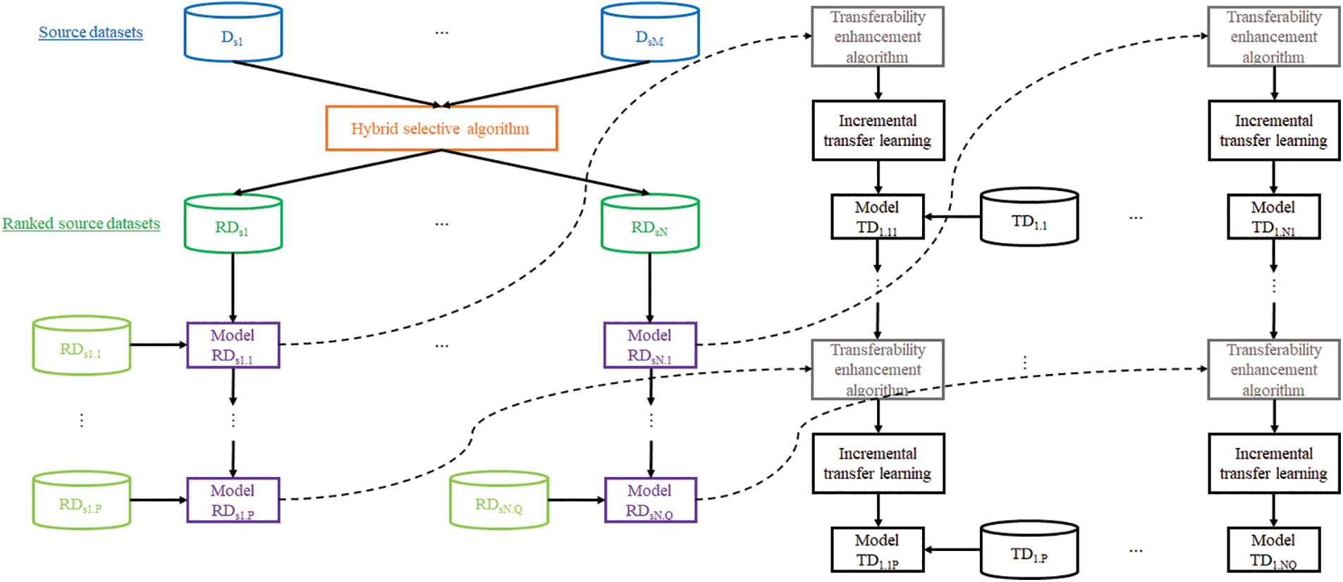
Figure 1: The architecture of our SA-ITL algorithm
If we have M sets of data from various sources (Ds1, ..., DsM) and one target dataset (TD), we can use a hybrid selective algorithm (as described in Subsection 2.2 B) to rank the similarities between the source and target datasets. The algorithm will output a descending order of ranked source datasets (RDs1, ..., RDsN), where the most similar dataset is listed first. It’s worth noting that N is less than M since some of the source datasets may not be relevant to the target domain and may be removed. Each ranked source dataset will be divided into some subsets, which need not be identical in size, using an incremental transfer learning algorithm. Each subset will train or update the models to form model RDs1.1, …, RDs1.P for the source dataset RDs1, which will continue until model RDsN.1, …, RDsN.Q for the source dataset RDsN is formed. Each of these models will undergo transferability enhancement (Subsection C) and incremental transfer learning (Subsection D) to update the target model, starting with TD1.11, …, TD1.1P using RDs1, and ending with TD1.N1, …, TD1.NQ using RDsN.
2.2 Hybrid Selective Algorithm Using Improved Dynamic Time Warping and Silhouette Coefficient
To prevent wasting time and resources on irrelevant knowledge transfer, as well as a reduction of the model’s performance, it is crucial to carefully select the appropriate source models. Negative transfer is a common issue that can arise from transferring irrelevant knowledge. Among the relevant source models, prioritizing the ones that share similarities with the target domain and transferring them in a one-to-one manner based on their descending order of similarities can be beneficial. During the initial iterations, the adoption of this approach can enhance the resilience of the target model. This, in turn, can mitigate the adverse impact of negative transfer from less analogous source domains in the subsequent iterations.
A hybrid approach is suggested to create a selective algorithm for multiple source models, which merges modified dynamic time warping (MDTW) and the Silhouette coefficient. Dynamic time warping (DTW) optimally aligns two time-series sequences on a similarity basis, but it is only effective when the sampling frequencies across multiple sensors are even [12]. MDTW is proposed to address this limitation by enabling uneven sampling frequencies that are commonly used in real-world scenarios. Our work builds on the Silhouette coefficient [13], which is used to select the source domains based on a pre-trained model and target domain. However, we extend this by incorporating the features of the source domains.
The formulation and design of the MDTW algorithm is explained as follows. The slopes (uphill and downhill) represent prominent information that helps evaluate the similarities between sequences. Particularly, the peaks that join the end of an uphill slope and the start of a downhill slope are of interest. The locations of the peaks are similar to the localizations of QRS complexes in the electrocardiogram signal.
The high-pass filter’ cut-off frequency fhigh and that of the low-pass filter flow are denoted, where fhigh<flow. These frequencies are chosen based on the frequencies of the sensors in the datasets. A derivative filter is applied to sharpen the uphill and downhill slopes. To further enhance the slopes, signal squaring is used. This is followed by moving window integration, with the difference equation as follows:
Two thresholds are defined to control the region of valid slopes, where the upper bound is
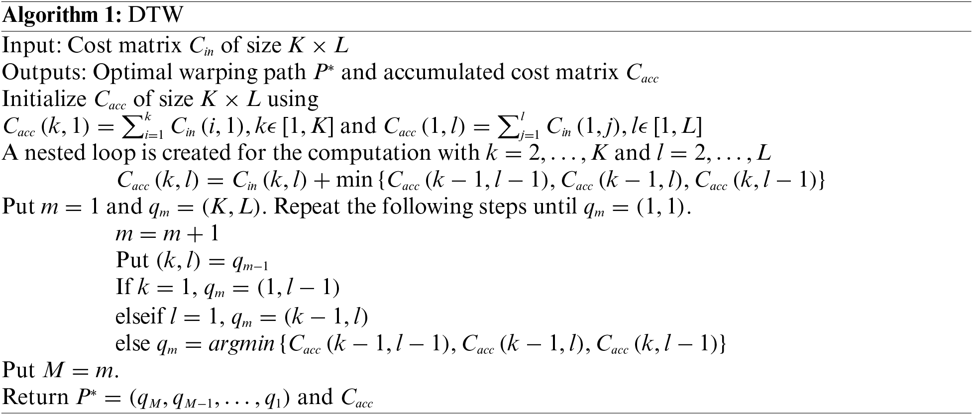
Obtaining the slopes is the first step, after which the standard DTW algorithm can be applied. To execute this algorithm, it is necessary to iterate through each dataset class and compute the mean of the time series for that class. This results in the creation of the DTW barycenter, which is then combined with the medoid of the time series set. This process is repeated for each pair of datasets, using one-to-one mapping. The distance between two datasets can be determined by the minimum DTW distance between their respective classes. The standard DTW algorithm is presented in Algorithm 1.
Consider datasets Di and Dj with sequences Ni and Nj, respectively. The total similarity score is defined as:
where
To determine the Silhouette coefficient, the training data sets are encoded using each source model before calculating the average coefficient (SC) for individual encodings.
with individual Silhouette coefficients SCi, the separation distance of encodings d, labels G and H, the final model’s label L, and the encoded labels’ length
After comparing the similarity scores of all pairs, they are adjusted and given weights based on the results obtained from the Silhouette coefficient. This process allows us to determine the priority order of the source domains to be transferred.
2.3 Transferability Enhancement Algorithm Using Three-Layer Scheme
Improvement of the target model’s performance is not always guaranteed with transfer learning, as negative transfer can occur. A recent study on negative transfer offered some common solutions to this issue [14]. These three categories are commonly used for transfer learning: (i) transferability enhancement, which involves improving the quality of data in the source datasets to enhance the transfer learning performance of the target model; (ii) distant transfer, which addresses the issue of low similarity between the source and target datasets, especially when they are related to different research topics. Some researchers have found that setting up an intermediate domain can be an effective way to bridge between the source-target domain; and (iii) secure transfer, which aims to ensure that the target model receives positive transfer by defining an appropriate objective function.
Enhancing the transferability of data between the source and target domains is better achieved through the first approach. The second approach is not suitable because it requires knowledge of experiences from the source domain that are difficult to obtain or that generate an intermediate domain. The last approach is not opted for because it demands an exhaustive understanding of all source domains and imposes restrictions on the formulation and design of the transfer learning problem. The data quality is enhanced using a three-layer architecture, which is designed to formulate the optimization problems in the domain-, instance-, and feature-layers. Fig. 2 summarizes the workflow of the three-layer scheme for transferability enhancement.
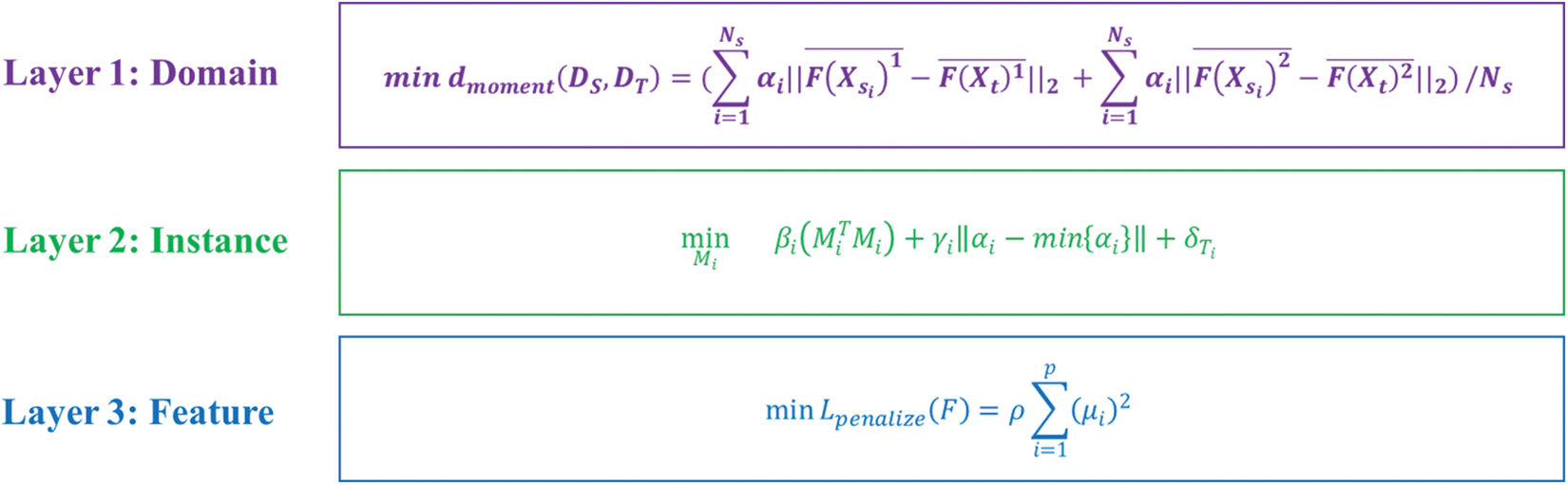
Figure 2: The workflow of the three-layer scheme for transferability enhancement
The similarity between two domains is measured in the domain layer by first considering the moment distance, represented by
with the average operations of the second-order features
Based on Eq. (11), it is assumed identical weighting factors for all source domains, which may not accurately reflect the differing levels of similarity between multiple source-target domains. To account for this, the modified moment distance, denoted as
with normalized weight
The instance layer focuses on transferring representative features between source-target domain. A transfer learning minimization problem can be formulated based on component Ci as follows:
with Mahalanobis distance Mi for Ci, the control factor
with the total of the weighted difference within classes
Regarding feature-layer, it is possible to lower the weighting factors of corresponding features with small singular values through the use of singular value decomposition (SVD). The feature matrix, denoted by
with the left singular vector U, the singular value matrix
with control factor
2.4 Incremental Transfer Learning
To leverage the models’ learning rate and reduce the impact of negative transfer on the target model, all source and target models are trained using incremental transfer learning. All datasets are divided into some subsets where the number of subsets needs to be determined for each dataset. The idea is explained as follows.
The model suffers from the poor transfer in the early rounds of model training because the model has only seen a relatively small portion of data. In the later rounds of model training, the model learns at a slower rate if the same amount of data is introduced in each round of training with the settings from an early round. The initial rate of training data is denoted as
The incremental transfer learning algorithm comprises the following key steps:
Step 1: Select one source dataset
Step 2: Divide
Step 3: Train model
Step 4: Train model
and sub-dataset
Step 5: Using
Step 6: Using
Step 7: Steps 5 and 6 are reapted with termination condition of all subsets are used.
3 Performance Evaluation and Comparison
The SA-ITL is evaluated using ten benchmark datasets. It is then compared with algorithms from existing works.
Seven of the benchmark datasets are machine fault-related datasets (as homogeneous datasets) and three are image datasets (as heterogeneous datasets). The details of the datasets are summarized here, with the first seven datasets being machine fault datasets.
(i) Case Western Reserve University (CWRU) dataset [15]: It comprises fan-end and single-point drive-end faults (ball faults, outer race faults, and inner race faults) as well as normal bearings. Data of drive-end bearings were collected using two sample rates of 48 k and 12 k samples/second, and that for collecting data of fan-end bearings was 12 k samples/second. The faults were based on artificial damage to the bearings.
(ii) Franche-Comté Électronique Mécanique Thermique et Optique—Sciences et Technologies (FEMTO-ST) dataset [16]: Seventeen run-to-failure data were sampled with 25.6 kHz under three operating settings. The experiment involved rotating, degradation generation, and measurement modules.
(iii) Paderborn University dataset [17]: In total, 32 ball-bearing experiments were conducted that covered 14 run-to-failure faults, 12 artificially damaged faults (inner and outer race faults), and 6 healthy operations. The sampling rate was 64 kHz. The experimental devices were a drive motor, a test module, a torque measurement shaft, and a load motor.
(iv) Machinery Failure Prevention Technology (MFPT) dataset [18]: Three experiments were conducted to measure vibration signals in healthy, inner, and outer race faults. Various loadings (25, 50, 100, 150, 200, 250, 270, and 300 lbs) were introduced. Two versions of the sampling rate were used; they were 97.656 kHz and 48.828 kHz.
(v) Center for Intelligent Maintenance Systems (IMS) dataset [19]: Three experiments were conducted on four bearings. The heavy loading of 6 k pounds was introduced to the bearings and shaft using a spring architecture. The sampling rate was chosen as 20 kHz.
(vi) Dynamic and Identification Research Group (DIRG) dataset [20]: Two experiments were carried out to collect data for high-speed (6 k rpm) aeronautical roller bearings. First, a bearing with singular damage was tested at a constant load and speed. Second, bearings with varying amounts of damage, such as a single roller fault and inner race fault, were tested at different loadings and speeds. Both experiments employed a sampling rate of 51.2 kHz.
(vii) PHM 2009 Gearbox dataset [21]: A gearbox was composed of six bearings, four gears, and three shafts. It has been used in experiments with varying gear types (helical and spur gears), loadings (high and low), and speeds (30, 35, 40, 45, and 50 Hz). The sampling frequency of the vibration signals was about 66.7 kHz.
(viii) ImageNet dataset [22]: This is one of the well-known (>40000 citations based on Google Scholar) and largest image datasets that consists of 1.28 million training images. It was used to demonstrate the transfer learning’s effectiveness in MFD [23].
(ix) CIFAR-10 dataset [24]: This is another image dataset with high citations (>16000 citations based on Google Scholar). It comprises 50 k and 10 k training and testing images, respectively.
(x) Microsoft Common Objects in Context (COCO) dataset [25]: Receiving much attention (>24000 citations based on Google Scholar), the COCO dataset consists of more than 328 k images that cover multidisciplinary research topics, including dense pose estimation, panoptic segmentation, stuff image segmentation, keypoint detection, natural language processing, and object detection.
3.2 Performance Evaluation of SA-ITL
The purpose of this research study was to investigate the adaptability and selectivity of the incremental transfer learning algorithm, with a focus on exploring research directions beyond feature extraction and classification algorithms. As a result, the target model utilizes a convolutional neural network as its foundational architecture.
To prevent overfitting and optimize the models accurately, a five-fold cross-validation technique is utilized. This technique is not uncommon, as justified in [26,27]. As there are ten standard datasets chosen, the target model undergoes nine rounds of SA-ITL at most, using nine source datasets. The training ceases when poor transfer is a large extent, i.e., when the target model performance (accuracy) is lower than the previous source dataset.
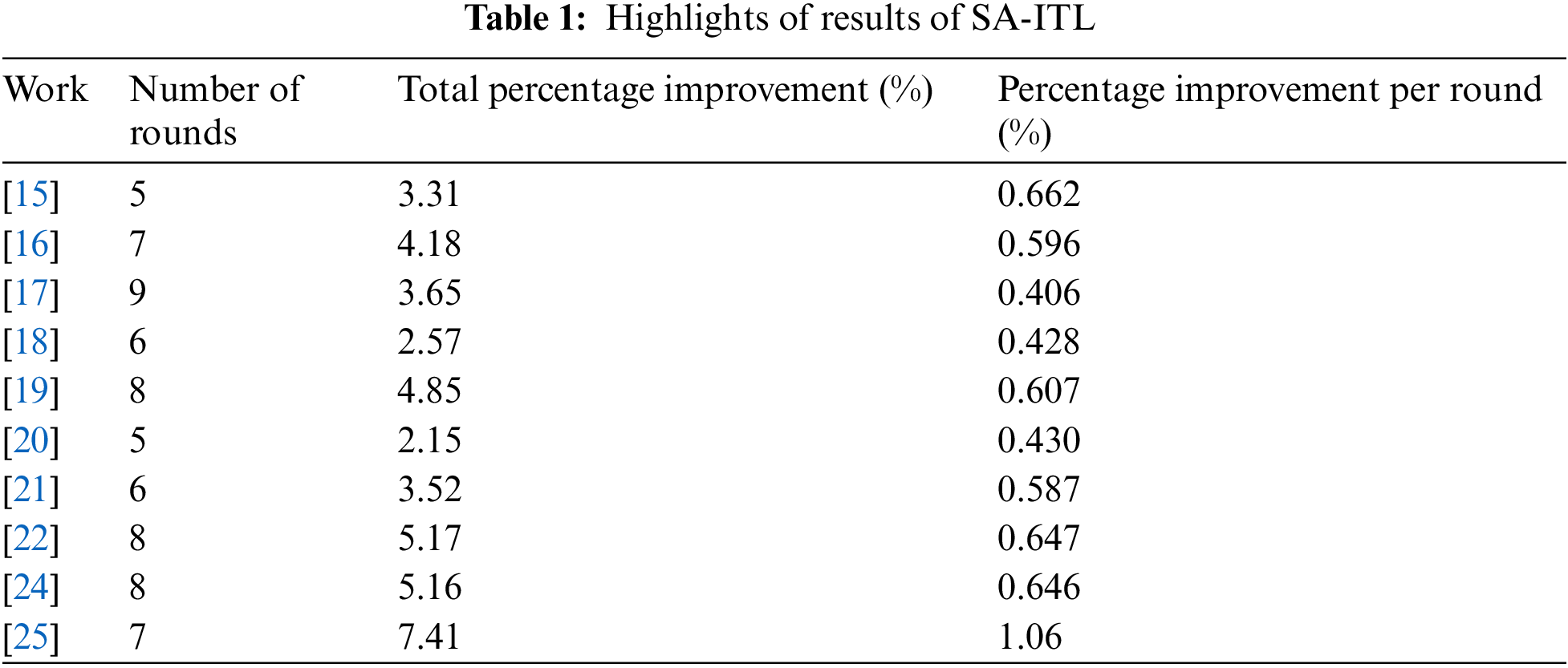
Fig. 3 illustrates how accurate the ten target models were in each round of SA-ITL. Out of those ten target models, eight managed to achieve an accuracy greater than 99%. However, the target model that utilized the ImageNet dataset achieved an accuracy of only 91.5%, and the target model that used the COCO dataset [25] was limited to an accuracy of 65.2%. Table 1 provides a summary of the number of rounds of SA-ITL that took place across the target models, the percentage of improvement between the first and last rounds of SA-ITL, and the percentage of improvement per round.
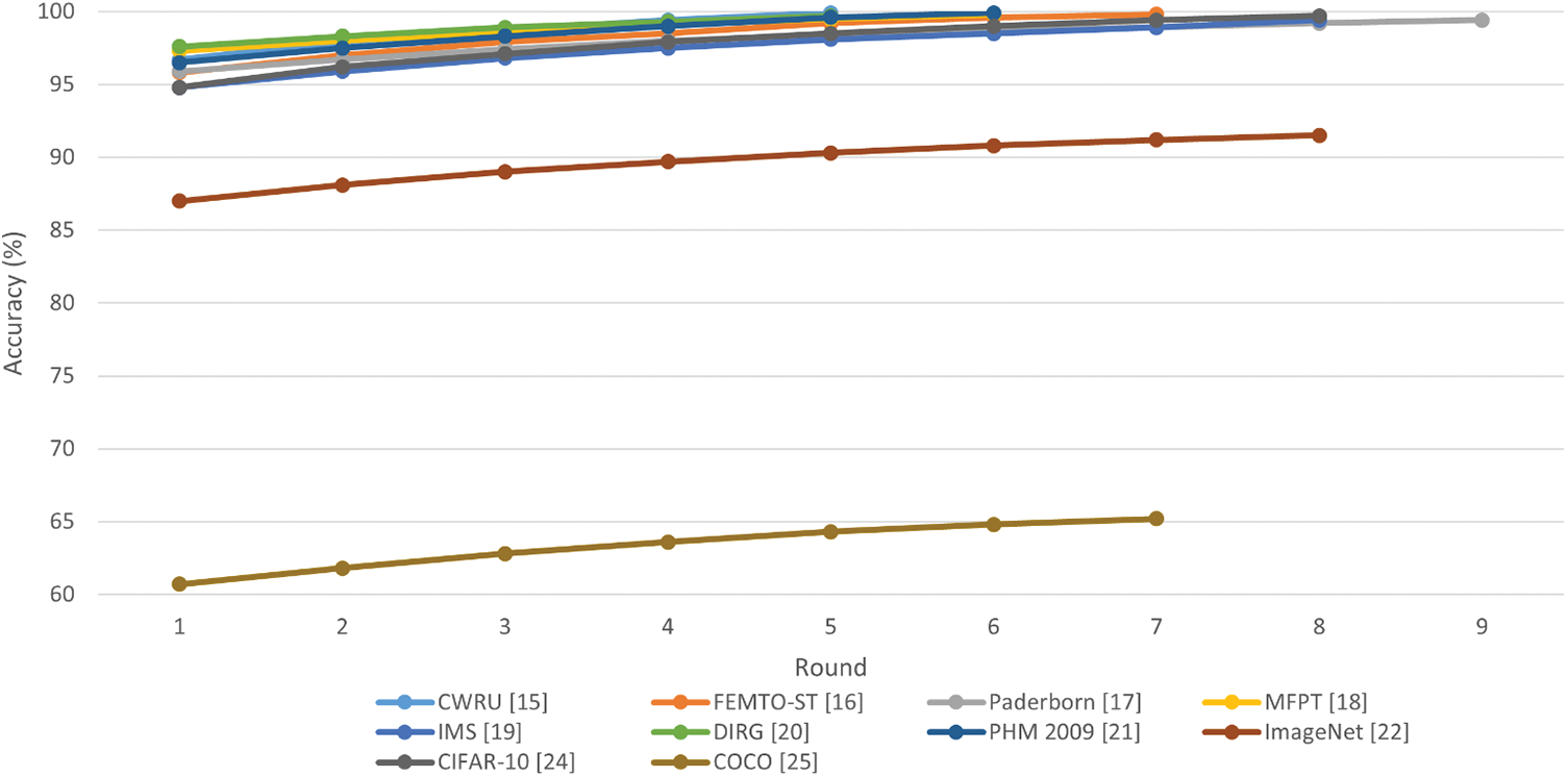
Figure 3: Performance of target models using multiple rounds of SA-ITL
3.3 Performance Comparison with Algorithms from Related Works
Table 2 compares the SA-ITL and related works.
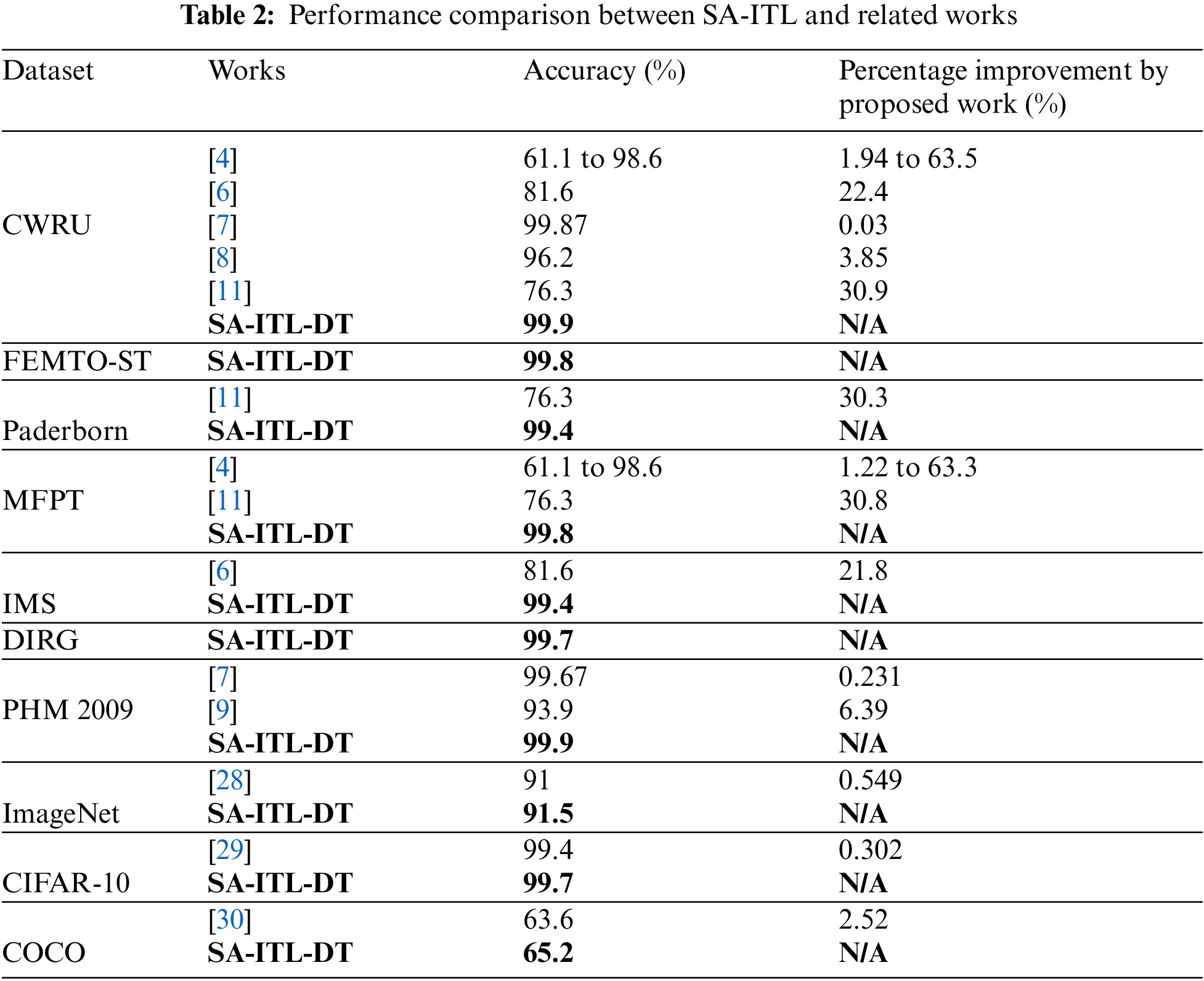
(i) The SA-ITL algorithm enhances the accuracy by 0.03%–63.0% for CWRU, 30.3% for Paderborn, 1.21%–63.3% for MFPT, 21.8% for IMS, 0.231%–6.39% for PHM 2009, 0.549% for ImageNet, 0.302% for CIFAR-10, and 2.52% for COCO.
(ii) It can be seen from the comparisons that some of the related works yielded an accuracy of more than 99%, while SA-ITL achieved a slight improvement. It is noted that the traditional CNN architecture is simpler than that in the proposals of the enhanced classification models in the related works.
Ablation studies are conducted on three essential components of SA-ITL in order to assess their advantages. These three key components include the hybrid selective algorithm, the transferability enhancement algorithm, and incremental transfer learning. The accuracy is compared between the scenarios where one of these components is removed and the scenario where none of the components are removed.
4.1 Benefits of Hybrid Selective Algorithm
Fig. 4 compares the accuracy of SA-ITL (with the hybrid selective algorithm) and A-ITL (without the hybrid selective algorithm). The percentage improvement by SA-ITL in each target model is ordered as follows: 3.82% for COCO, 2.92% for ImageNet, 2.69% for Paderborn, 2.36% for CWRU, 1.94% for FEMTO-ST, 1.59% for IMS, 1.55% for DIRG, 1.52% for MFPT, 1.42% for PHM 2009, and 1.22% for CIFAR-10. The results can be explained by a key factor, in which A-IT without a hybrid selective algorithm (and with fewer source datasets) will end earlier due to the increasing chance of negative transfer.
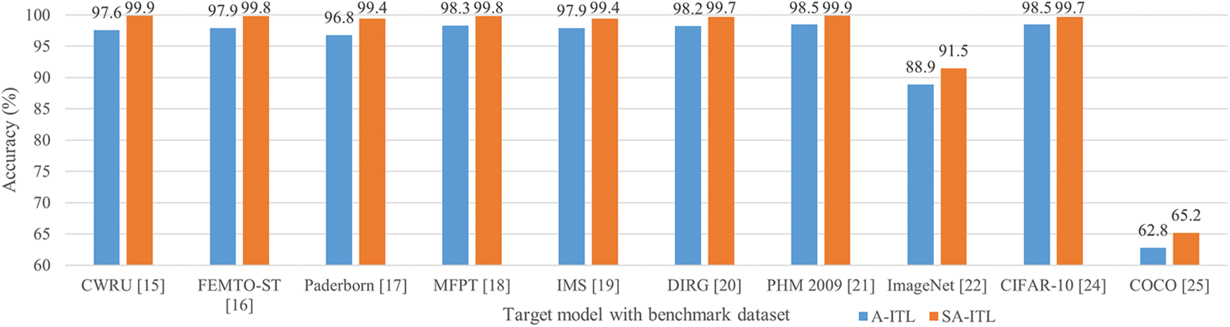
Figure 4: Performance comparison between A-ITL and SA-ITL
4.2 Benefits of Transferability Enhancement Algorithm
The accuracies of SA-ITL (with the transferability enhancement algorithm) and S-ITL (without the transferability enhancement algorithm) are shown in Fig. 5. The percentage improvement by SA-ITL in the target model is ordered as follows: 4.15% for COCO, 3.62% for ImageNet, 3.22% for Paderborn, 2.78% for CWRU, 2.59% for CIFAR-10, 2.55% for MFPT, 2.25% for FEMTO-ST, 1.95% for IMS, 1.94% for DIRG, and 1.91% for PHM 2009. The results suggest that the transferability enhancement in the domain, instance, and feature layers facilitates the knowledge transfer between source-target domain.
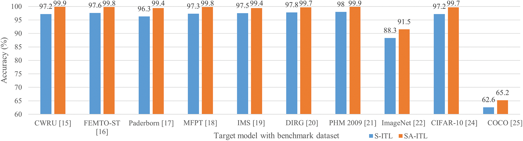
Figure 5: Performance comparison between S-ITL and SA-ITL
4.3 Benefits of Incremental Transfer Learning
The accuracies of SA-ITL (with incremental transfer learning) and SA-TL (without incremental transfer learning) are shown in Fig. 6.
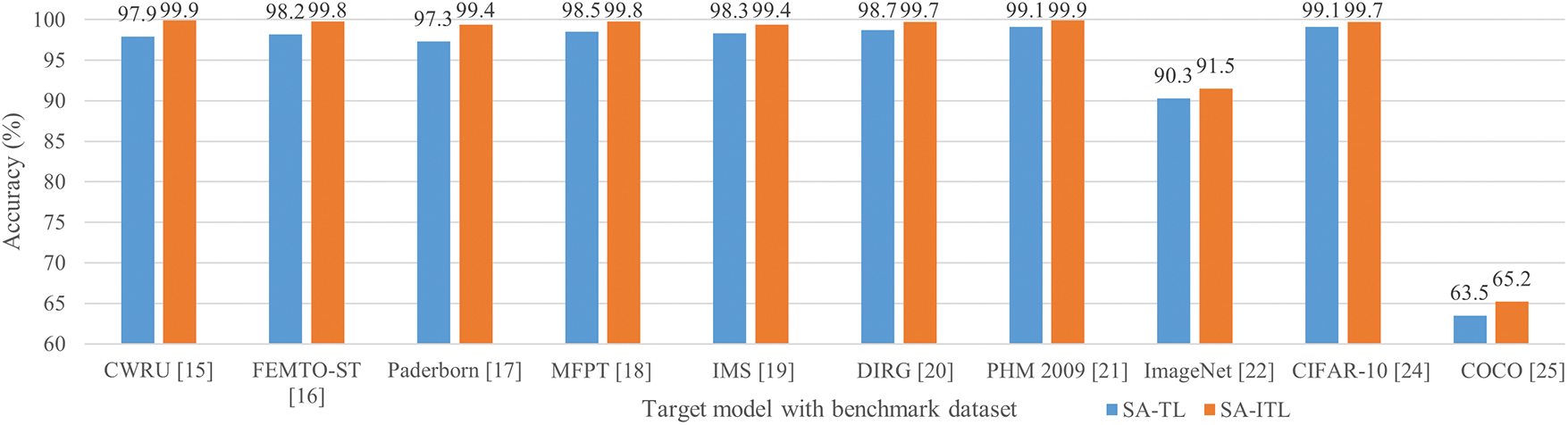
Figure 6: Performance comparison between SA-TL and SA-ITL
The percentage improvement by SA-ITL in the target model is ordered as follows: 2.68% for COCO, 2.16% for Paderborn, 2.04% for CWRU, 1.63% for FEMTO-ST, 1.33% for ImageNet, 1.32% for MFPT, 1.12% for IMS, 1.01% for DIRG, 0.807% for PHM 2009, and 0.605% for CIFAR-10. The results verify the effectiveness of dividing the whole dataset into several subsets for increment transfer learning.
4.4 Summary of Ablation Studies
The ablation studies revealed accuracy enhancements of 1.22%–3.82% for the hybrid selective algorithm, 1.91%–4.15% for the transferability enhancement algorithm, and 0.605%–2.68% for the incremental transfer learning algorithm. Therefore, individual techniques, including hybrid selective algorithm, transferability enhancement algorithm, and incremental transfer learning algorithm, are essential to enhance the accuracy of the machine fault diagnosis problems.
5 Conclusion and Future Research Directions
This paper proposed SA-ITL to enhance the effectiveness of transfer learning. Three algorithms were adopted.
First, a hybrid selective algorithm helped prioritize relevant source datasets to transfer them to the target model. Second, a transferability enhancement algorithm enhanced the knowledge transfer with a three-layer perspective containing the domain, instance, and feature layers. Last, incremental transfer learning divided the source and target datasets into several subsets of lower computational complexity and balanced the learning rate and negative transfer avoidance. The performance evaluation shows that SA-ITL yields an accuracy of at least 99.4% when using eight benchmark datasets and will be improved significantly with the remaining two. The comparison reveals that SA-ITL outperforms other algorithms from existing works by 0.03%–63.3%. It also shows the ability of transfer learning to work with heterogeneous image datasets, where the robustness of the models is enhanced with large-scale datasets. Regarding the necessity of the three components of SA-ITL, ablation studies are carried out to remove one of the components in each experiment. The improvement in the average accuracies with the 10 benchmark datasets is 2.10%, 2.70%, and 1.47%, respectively.
The authors understand that there are research limitations that require further investigation. Future research directions are explained as follows: First, evaluate the SA-ITL using other base algorithms (a CNN was used in this research work) such as a deep belief network [31] and a dual convolutional capsule CNN [32]. Second, extend the disciplines of the benchmark datasets for distant transfer learning (can be heterogeneous, such as in current research works that have selected two machine fault diagnosis and image datasets) [33,34]. Third, investigate how effectively the model will perform when replacing the weighting factors of the source datasets with a set of hyperparameters to be optimized in the objective functions [35,36]. Last, introduce fault-tolerance algorithms to recover from failures [37,38].
Acknowledgement: Not applicable.
Funding Statement: The authors received no specific funding for this study.
Author Contributions: The authors confirm contribution to the paper as follows: study conception and design: Kwok Tai Chui, Brij B. Gupta; analysis and interpretation of results: Kwok Tai Chui, Brij B. Gupta, Varsha Arya, Miguel Torres-Ruiz; draft manuscript preparation: Kwok Tai Chui, Brij B. Gupta, Varsha Arya, Miguel Torres-Ruiz. All authors reviewed the results and approved the final version of the manuscript.
Availability of Data and Materials: Not applicable.
Conflicts of Interest: The authors declare that they have no conflicts of interest to report regarding the present study.
References
1. A. Abid, M. T. Khan and J. Iqbal, “A review on fault detection and diagnosis techniques: Basics and beyond,” Artificial Intelligence Review, vol. 54, no. 5, pp. 3639–3664, 2021. [Google Scholar]
2. H. Zheng, R. Wang, Y. Yang, J. Yin, Y. Li et al., “Cross-domain fault diagnosis using knowledge transfer strategy: A review,” IEEE Access, vol. 7, pp. 129260–129290, 2019. [Google Scholar]
3. W. Li, R. Huang, J. Li, Y. Liao, Z. Chen et al., “A perspective survey on deep transfer learning for fault diagnosis in industrial scenarios: Theories, applications and challenges,” Mechanical Systems and Signal Processing, vol. 167, pp. 108487, 2022. [Google Scholar]
4. Y. Dong, Y. Li, H. Zheng, R. Wang and M. Xu, “A new dynamic model and transfer learning based intelligent fault diagnosis framework for rolling element bearings race faults: Solving the small sample problem,” ISA Transactions, vol. 121, pp. 327–348, 2022. [Google Scholar] [PubMed]
5. L. Chen, Q. Li, C. Shen, J. Zhu, D. Wang et al., “Adversarial domain-invariant generalization: A generic domain-regressive framework for bearing fault diagnosis under unseen conditions,” IEEE Transactions on Industrial Informatics, vol. 18, no. 3, pp. 1790–1800, 2022. [Google Scholar]
6. L. Wan, Y. Li, K. Chen, K. Gong and C. Li, “A novel deep convolution multi-adversarial domain adaptation model for rolling bearing fault diagnosis,” Measurement, vol. 191, pp. 110752, 2022. [Google Scholar]
7. J. Tian, D. Han, M. Li and P. Shi, “A multi-source information transfer learning method with subdomain adaptation for cross-domain fault diagnosis,” Knowledge-Based Systems, vol. 243, pp. 108466, 2022. [Google Scholar]
8. X. Li and W. Zhang, “Deep learning-based partial domain adaptation method on intelligent machinery fault diagnostics,” IEEE Transactions on Industrial Electronics, vol. 68, no. 5, pp. 4351–4361, 2021. [Google Scholar]
9. M. Deng, A. Deng, Y. Shi, Y. Liu and M. Xu, “A novel sub-label learning mechanism for enhanced cross-domain fault diagnosis of rotating machinery,” Reliability Engineering & System Safety, vol. 225, pp. 108589, 2022. [Google Scholar]
10. S. Liu, H. Wang, J. Tang and X. Zhang, “Research on fault diagnosis of gas turbine rotor based on adversarial discriminative domain adaption transfer learning,” Measurement, vol. 196, pp. 111174, 2022. [Google Scholar]
11. H. Zheng, Y. Yang, J. Yin, Y. Li, R. Wang et al., “Deep domain generalization combining a priori diagnosis knowledge toward cross-domain fault diagnosis of rolling bearing,” IEEE Transactions on Instrumentation and Measurement, vol. 70, pp. 1–11, 2021. [Google Scholar]
12. H. Hamedi, R. Shad and S. Jamali, “Measuring lane-changing trajectories by employing context-based modified dynamic time warping,” Expert Systems with Applications, vol. 216, pp. 119489, 2023. [Google Scholar]
13. A. Meiseles and L. Rokach, “Source model selection for deep learning in the time series domain,” IEEE Access, vol. 8, pp. 6190–6200, 2020. [Google Scholar]
14. W. Zhang, L. Deng, L. Zhang and D. Wu, “A survey on negative transfer,” IEEE/CAA Journal of Automatica Sinica, vol. 10, no. 2, pp. 305–329, 2023. [Google Scholar]
15. Case Western Reserve University Bearing Data Center, “Bearing data center,” [Online]. Available: https://engineering.case.edu/bearingdatacenter/download-data-file (accessed on 20/07/2023). [Google Scholar]
16. P. Nectoux, R. Gouriveau, K. Medjaher, E. Ramasso, B. Chebel-Morello et al., “PRONOSTIA: An experimental platform for bearings accelerated degradation tests,” in IEEE Int. Conf. on Prognostics and Health Management, Denver, USA, pp. 1–8, 2012. [Google Scholar]
17. C. Lessmeier, J. K. Kimotho, D. Zimmer and W. Sextro, “Condition monitoring of bearing damage in electromechanical drive systems by using motor current signals of electric motors: A benchmark data set for data-driven classification,” in PHM Society European Conf., Bilbao, Spain, pp. 1–17, 2016. [Google Scholar]
18. Society For Machinery Failure Prevention Technology, “Fault data sets,” 2013. [Online]. Available: https://www.mfpt.org/fault-data-sets/ (accessed on 20/07/2023). [Google Scholar]
19. H. Qiu, J. Lee, J. Lin and G. Yu, “Robust performance degradation assessment methods for enhanced rolling element bearing prognostics,” Advanced Engineering Informatics, vol. 17, no. 3–4, pp. 127–140, 2003. [Google Scholar]
20. A. P. Daga, A. Fasana, S. Marchesiello and L. Garibaldi, “The Politecnico di Torino rolling bearing test rig: Description and analysis of open access data,” Mechanical Systems and Signal Processing, vol. 120, pp. 252–273, 2019. [Google Scholar]
21. PHM Society, “Data analysis competition,” 2009. [Online]. Available: https://www.phmsociety.org/competition/PHM/09 (accessed on 20/07/2023). [Google Scholar]
22. J. Deng, W. Dong, R. Socher, L. J. Li, K. Li et al., “Imagenet: A large-scale hierarchical image database,” in 2009 IEEE Conf. on Computer Vision and Pattern Pattern Recognition, Miami, USA, pp. 248–255, 2009. [Google Scholar]
23. S. Shao, S. McAleer, R. Yan and P. Baldi, “Highly accurate machine fault diagnosis using deep transfer learning,” IEEE Transactions on Industrial Informatics, vol. 15, no. 4, pp. 2446–2455, 2019. [Google Scholar]
24. A. Krizhevsky, “Learning multiple layers of features from tiny images,” Master’s Thesis, University of Toronto, Canada, 2009. [Google Scholar]
25. T. Y. Lin, M. Maire, S. Belongie, J. Hays, P. Perona et al., “Microsoft COCO: Common objects in context,” in Computer Vision–ECCV 2014: 13th European Conf., Zurich, Switzerland, pp. 740–755, 2014. [Google Scholar]
26. L. Zuo, F. Xu, C. Zhang, T. Xiahou and Y. Liu, “A multi-layer spiking neural network-based approach to bearing fault diagnosis,” Reliability Engineering & System Safety, vol. 225, pp. 108561, 2022. [Google Scholar]
27. L. Wen, X. Xie, X. Li and L. Gao, “A new ensemble convolutional neural network with diversity regularization for fault diagnosis,” Journal of Manufacturing Systems, vol. 62, pp. 964–971, 2022. [Google Scholar]
28. J. Yu, Z. Wang, V. Vasudevan, L. Yeung, M. Seyedhosseini et al., “Coca: Contrastive captioners are image-text foundation models,” arXiv preprint arXiv:2205.01917, 2022. [Google Scholar]
29. H. Touvron, M. Cord, A. Sablayrolles, G. Synnaeve and H. Jégou, “Going deeper with image transformers,” in Proc. of the IEEE/CVF Int. Conf. on Computer Vision, Montreal, Canada, pp. 32–42, 2021. [Google Scholar]
30. H. Zhang, F. Li, S. Liu, L. Zhang, H. Su et al., “DINO: DETR with improved denoising anchor boxes for end-to-end object detection,” arXiv preprint arXiv:2203.03605, 2022. [Google Scholar]
31. H. Zhao, J. Liu, H. Chen, J. Chen, Y. Li et al., “Intelligent diagnosis using continuous wavelet transform and gauss convolutional deep belief network,” IEEE Transactions on Reliability, vol. 72, no. 2, pp. 692–702, 2023. [Google Scholar]
32. D. Li, M. Zhang, T. Kang, B. Li, H. Xiang et al., “Fault diagnosis of rotating machinery based on dual convolutional-capsule network (DC-CN),” Measurement, vol. 187, pp. 110258, 2022. [Google Scholar]
33. W. He, J. Chen, Y. Zhou, X. Liu, B. Chen et al., “An intelligent machinery fault diagnosis method based on GAN and transfer learning under variable working conditions,” Sensors, vol. 22, no. 23, pp. 9175, 2022. [Google Scholar] [PubMed]
34. C. Li, S. Zhang, Y. Qin and E. Estupinan, “A systematic review of deep transfer learning for machinery fault diagnosis,” Neurocomputing, vol. 407, pp. 121–135, 2022. [Google Scholar]
35. J. Liang, Y. Liao, Z. Chen, H. Lin, G. Jin et al., “Intelligent fault diagnosis of rotating machinery using lightweight network with modified tree-structured parzen estimators,” IET Collaborative Intelligent Manufacturing, vol. 4, no. 3, pp. 194–207, 2022. [Google Scholar]
36. H. D. Shao, Z. Y. Ding, J. S. Cheng and H. K. Jiang, “Intelligent fault diagnosis among different rotating machines using novel stacked transfer auto-encoder optimized by PSO,” ISA Transactions, vol. 105, pp. 308–319, 2020. [Google Scholar]
37. F. A. Osuolale, “Reactive hybrid model for fault mitigation in real-time cloud computing,” International Journal of Cloud Applications and Computing, vol. 12, no. 1, 2022. [Google Scholar]
38. S. Jaswal and M. Malhotra, “AFTTM: Agent-based fault tolerance trust mechanism in cloud environment,” International Journal of Cloud Applications and Computing, vol. 12, no. 1, 2022. [Google Scholar]
Cite This Article
 Copyright © 2024 The Author(s). Published by Tech Science Press.
This work is licensed under a Creative Commons Attribution 4.0 International License , which permits unrestricted use, distribution, and reproduction in any medium, provided the original work is properly cited.
 Downloads
 Citation Tools