Improved Data Stream Clustering Method: Incorporating KD-Tree for Typicality and Eccentricity-Based Approach

1  Introduction

Clustering, a prominent research direction in data mining, is crucial in grouping data based on similarity. The application of clustering technology extends to various domains, including data mining, pattern recognition, and image processing. Different clustering algorithms possess distinct characteristics and are suitable for specific application scenarios.

However, it is essential to note that no single clustering algorithm can effectively address all clustering problems. Traditional clustering algorithms typically require a prior understanding of the dataset and rely on pre-training and adjustment based on specific dataset attributes. These methods are all targeted towards static datasets, assuming the dataset is complete and can be analyzed. However, as technology advances, data in various domains is no longer static but arrives incrementally over time. Such continuously arriving data is referred to as a data stream. Generally, as data volume increases, data stream clustering algorithms may encounter higher computational demands. Most existing data stream clustering algorithms exhibit a gradual increase in the time required for algorithm execution as data volume grows. Therefore, when dealing with large-scale data streams, the design and optimization of algorithms become particularly crucial. This paper aims to refine existing data stream clustering algorithms, improving the accuracy of clustering results and the efficiency of clustering, and propose an efficient data stream clustering algorithm that shows minimal changes in runtime with increasing data volume, making it more suitable for research in the clustering analysis of large-scale data streams.

After research and consideration, we choose the TEDA algorithm for improvement. TEDA algorithm is a developing anomaly detection method introduced by [1] TEDA algorithm counts some attributes of the cluster, such as variance, mean, etc., to put the data into the appropriate cluster or merge the clusters. The TEDA algorithm exhibits distinctive features, such as complete autonomy, adaptability to evolution, and computational simplicity. It can identify clusters of arbitrary shapes and requires the adjustment of only a single parameter to control the incorporation of data points into clusters. Despite these advantages, the algorithm faces challenges in data processing. Upon the arrival of new data points, it must traverse all existing clusters, increasing processing time as the data stream grows. Existing clusters continue accumulating with the growing data stream, escalating the time required to process newly arrived data points. However, new data points only need to enter clusters close to them in this process. Operating on all existing clusters significantly reduces the algorithm’s efficiency, causing a rapid increase in runtime with data volume growth.

In addressing this issue, we utilized various nearest-neighbor search algorithms to optimize the TEDA algorithm. Following experimental analysis, our final choice was integrating the KD-Tree (K-Dimensional Tree) algorithm with the Scapegoat Tree. This involves using the KD-Tree algorithm to identify the nearest cluster to the current data point, concurrently optimizing the KD-Tree with the Scapegoat Tree. The process continues to search for clusters based on distance. When multiple clusters are no longer suitable for incorporating new data points, the operation halts, awaiting the entry of the following data point. This optimization significantly improves the algorithm’s efficiency. Through experiments, it is evident that the algorithm’s runtime demonstrates a close-to-linear relationship with the data volume, rendering it highly suitable for large-scale data stream clustering analysis.

The contribution and innovation of this study can be summarized as follows:

1. The combined algorithm also features the original TEDA algorithm, which can recognize data of any shape and in any order and only needs to adjust the parameters to control the clustering results, with each data needing to be processed only once.

2. The combined algorithm focuses the clustering process more on the operations between data points and similar clusters through the KD-Tree algorithm. From the experimental results in Section 5, it can be seen that the runtime of the original TEDA algorithm increases exponentially with the growth of data. In contrast, the improved algorithm’s runtime is closer to a linear relationship. In other words, as the data increases, the time required to process each data point remains nearly constant. This significantly enhances the efficiency of the algorithm.

3. The KD-Tree algorithm can effectively reduce the impact of “dimension disaster” in high-dimensional data, and the combined algorithm has more advantages in processing high-dimensional data.

4. The combined algorithm can prevent the same data point from joining too many clusters to a certain extent. This can, to some extent, prevent the merging of two clusters with high overlap and improve the accuracy of clustering results.

This paper is structured as follows: Section 2 presents some algorithms that have been used in recent years in data stream clustering. Section 3 briefly describes the TEDA process. Section 4 summarizes the development of the proposed hybrid ensemble data stream clustering method. The experimental results and discussions are elaborated in Section 5. Finally, Section 6 is devoted to conclusions and future recommendations.

2  Related Works

The existing data stream clustering methods mainly include partitioning, hierarchical, density-based, grid-based, model-based, and other algorithms. Among the partitioning clustering methods, O’Callaghan et al. proposed STREAM [2] algorithm. Based on the k-medoids algorithm, processes the data in one data block at a time by decomposing the entire data stream into continuous data blocks. Aggarwal et al. proposed CluStream [3] algorithm, in which a famous online and offline two-phase framework is used. In recent studies, Li et al. proposed a complete granularity partitioning framework, RCD+ (Runtime Correlation Discovery) [4]. It partitions the compatibility data streams based on the pane and determines the candidate set of partitioning keys in the static compilation stage of query processing. Liu et al. proposed a novel space partitioning algorithm, called EI-kMeans (Equal Intensity kMeans) [5], for drift detection on multicluster datasets. EI-kMeans is a modified K-Means algorithm to search for the best centroids to create partitions. Alotaibi proposed a new meta-heuristics algorithm based on Tabu Search and K-Means, called MHTSASM (Meta-Heuristics Tabu Search with an Adaptive Search Memory) [6]. The proposed algorithm overcomes the initialization sensitivity of K-Means and reaches the global optimal effectively.

Among the hierarchical clustering methods, Zhang et al. proposed BIRCH (Balanced Iterative Reducing and Clustering using Hierarchies) [7] algorithm for large-scale data clustering. This algorithm can effectively cluster with one-pass scanning and deal with outliers. In recent studies, Cheung et al. proposed a fast and accurate hierarchical clustering algorithm based on topology training called GMTT (Growing Multilayer Topology Training) [8]. A trained multilayer topological structure that fits the spatial distribution of the data is utilized to accelerate the similarity measurement, which dominates the computational cost in hierarchical clustering. Sangma et al. [9] proposed a hierarchical clustering technique for multiple nominal data streams. The proposed technique can address the concept-evolving nature of the data streams by adapting the clustering structure with the help of merge and split operations. Nikpour et al. proposed a new incremental learning-based method, called DCDSCD (Dynamic Clustering of the Data Stream with considering Concept Drift) [10], which is an incremental supervised clustering algorithm. In the proposed algorithm, the data stream is automatically clustered in a supervised manner, where the clusters whose values decrease over time are identified and then eliminated.

Among the density-based clustering methods, Cao et al. proposed DenStream [11] algorithm, it combines DBSCAN and the previously mentioned two-phase framework and overcomes the disadvantage that the CluStream algorithm is insensitive to noise. In recent studies, Amini et al. proposed a multi-density data stream clustering algorithm called MuDi-Stream (Multi Density data Stream) [12]. In this algorithm, a hybrid method based on grid and micro clustering is used to extract data information and reduce the merging time of data clustering. Laohakiat et al. proposed LLDstream [13] algorithm. In this study, a dimension reduction technique called ULLDA (Unsupervised Localized Linear Discriminant Analysis) is proposed and incorporated into the framework of data stream clustering. Islam proposed a completely online density-based clustering algorithm, called buffer-based online clustering for evolving data stream, called BOCEDS (Buffer-based Online Clustering for Evolving Data Stream) [14]. The algorithm recursively updates the micro cluster radius to the optimal location. Faroughi et al. proposed ARD-Stream (Adaptive Radius Density-based Stream clustering) [15], in this study, by considering both the shared density and distance between micro-clusters, leading to more accurate clusters.

Among the grid-based clustering methods, Ntoutsi et al. proposed D-Stream [16] algorithm, it is an improvement on the Den Stream algorithm, which divides the entire data space according to dimensions, and stores the summary information of data objects in the cell grid. In recent studies, Bhatnagar et al. proposed an Exclusive and Complete Clustering algorithm that captures non-overlapping clusters in data streams with mixed attributes called ExCC (Exclusive and Complete Clustering) [17], such that each point either belongs to some cluster or is an outlier/noise. Chen et al. proposed a novel fast and grid-based clustering algorithm for the hybrid data stream called FGCH (Fast and Grid based Clustering algorithm for Hybrid data stream) [18]. They developed a non-uniform attenuation model to enhance the resistance to noise,proposed a similarity calculation method for hybrid data, which can calculate the similarity more efficiently and accurately. Tareq et al. proposed a new online method, which is a density grid-based method for data stream clustering, called CEDGM (Clustering of Evolving Data streams via a density Grid-based Method) [19]. The primary objectives of the density grid-based method are to reduce the number of distant function calls and to improve cluster quality. Hu et al. proposed MDDSDB-GC (Multi-Density DBSCAN Based on Grid and Contribution) [20]. In this algorithm, the calculation methods of contribution, grid density, and migration factor are effectively improved.

Among the model-based clustering methods, Yang et al. proposed EM (Expectation and Maximization) [21] algorithm, its main idea is to replace a hard to handle likelihood function maximization problem with a sequence that is easy to maximize, and its limit is the solution to the original problem. Ghesmoune et al. proposed a new algorithm for online topological clustering of data streams called G-Stream (Growing Neural Gas over Data Streams) [22]. The algorithm only needs to process all the data once and determines the final class of the data by considering the topology of the data. Wattanakitrungroj et al. proposed a data stream clustering algorithm based on a new hyperelliptic function parameter updating and merging, which is called BEstream (Batch capturing with Elliptic function for One-Pass Data Stream Clustering) [23] algorithm. This algorithm does not need to process one data at a time. Nguyen et al. proposed an incremental online multi-label classification method based on a weighted clustering model called OMLC (Online Multi-Label Classification) [24]. The model adapts to the changes in data through an attenuation mechanism so that the weight of the achieved data will decrease with time.

3  TEDA

In this section, we focus on the process of the original TEDA algorithm and some of the current shortcomings of the TEDA algorithm.

3.1 TEDA Process

TEDA is a developing method for detecting anomalies and outliers introduced by Angelov in the article [1]. The concepts of typicality and eccentricity proposed in this paper have been successfully applied to data classification and other problems.

Typicality represents the similarity between a specific n-dimensional data sample and its past readings. Eccentricity describes the dispersion between a data sample and the data distribution center. Therefore, a data sample with high eccentricity, that is, low typicality, is usually an outlier [25].

Eccentricity is defined as the sum of the distances between a data sample and all other existing data samples divided by the sum of the distances between all data samples and all other data samples [25]. The calculation formula and value range are as follows:

ξk(x)=2∑i=1kd(x,xi)∑i=1k∑j=1kd(xi,xj),k≥2,∑i=1kd(x,xi)>0(1)

0≤ξk(x)≤1,∑i=1kξk(xi)=2(2)

In formula (1), ξk(x) is eccentricity. The existing research shows that for the calculation of Euclidean distance, the eccentricity calculation formula can be accurately deduced as:

ξ(xk)=1k+(μxk−xk)T(μxk−xk)k[σ2]xk(3)

In formula (3), k is the amount of data, μk is the average of all data samples, xk is the kth data, [σ2]xk is variance.

The typicality calculation formula is:

τ(xk)=1−ξ(xk)(4)

In formula (4), τ(xk) is typicality. Similar to eccentricity, the typical range is:

0≤τk(x)≤1,∑i=1kτk(xi)=k−2,k≥2(5)

Most of the time, we use its normalized version:

ζk(x)=ξk(x)2,∑i=1kζk(xi)=1,k≥2(6)

tk(x)=τk(x)k−2,∑i=1kτk(xi)=1,k>2(7)

In formulas (6) and (7), ζk(x) is the normalized eccentricity and tk(x) is the normalized typicality.

After introducing the concepts of typicality and eccentricity, we will explain the operation process of the TEDA algorithm in detail.

First, start reading the data. When the first data x1 enters, create cloud1, add x1 to cloud1, and initialize the attributes of cloud1 as:

s11=1μ11=x1[σ2]11=0

where s11 represents the quantity of all data contained in cloud1 when the first data arrived, μ11 represents the mean value of data in cloud1 at the time, and [σ2]11 represents the variance in cloud1 at the time [26].

When the first data enters successfully, continue to read the data. When the second data enters, put x2 into the existing cloud1 and update the attribute of cloud1 as:

s21=2(8)

μ21=(s21−1s21)×μ11+(1s21)×x2(9)

[σ2]21=(s21−1s21)×[σ2]11+(1s21−1)×‖x2−μ21‖2(10)

When the xk (k ≥ 3) data enters, try to put xk into all existing cloudi in turn, and calculate the temporary value of its attribute for cloudi’:

[ski] ′=[sk−1i]+1(11)

[μki] ′=[ski] ′−1[ski] ′×μk−1i+1[ski] ′×xk(12)

[[σ2]ki] ′=[ski] ′−1[ski] ′×[σ2]k−1i+1[ski] ′−1×‖xk−[μki] ′‖2(13)

Calculate its eccentricity and normalized eccentricity, ζk(x), at the same time, and use Chebyshev inequality:

ζk(x)>m2+12k,m>0(14)

In formula (14), m is the standard deviation distance of the data from the center value. If the data meets the Chebyshev inequality [27], it means that the eccentricity of xk to cloudi’ is too high and the typicality is too low. It is not suitable to join cloudi’. The attribute of cloudi’ needs to be returned. And the same data xk can be added to multiple cloudi’. If all the cloudi’ have been traversed, but there is no appropriate cloudi’ to add data xk, then create a new cloud and add data xk into it.

3.2 Disadvantages of the Original TEDA Algorithm

Nowadays, most of the existing clustering algorithms have their advantages and limitations. TEDA algorithm is one of the simple and efficient algorithms, but it also has the following problems:

1.    In Chebyshev inequality, m is usually a constant value of 3. When the amount of data is small, the average value and variance of the cloud are not accurate. Determining that data xk is m standard deviation from the cloud center value is difficult. Especially when x2 enters, the algorithm often directly adds the data to cloud1, which may lead to poor quality of the first few clouds [28].

2.    When new data arrives, the data point needs to be added to all existing clouds for judgment. When the data volume is large, there may be many clouds, and most clouds are far away from the data point, so it is unnecessary to add the data point, which will waste much time.

To solve the above problem 1, Maia et al. adjusted the value of m according to the number of incoming data, which improved the accuracy of the algorithm [28]. In this paper, the KD-Tree algorithm combined with the Scapegoat Tree is mainly used to improve the above problem 2.

4  NS-TEDA Approach

In the TEDA algorithm, when each data point enters, it is necessary to put it into all the existing clouds and then use Chebyshev’s inequality to determine whether the data point is suitable to join a certain cloud. In a discrete dataset, there may be many clouds distributed throughout the data space, when a new data point enters, it will only join the clouds that are close to it. However, in the original TEDA algorithm, operations are performed on all existing clouds, which may involve a significant number of steps that could be omitted. Therefore, we try to use nearest neighbor search related algorithms, such as KD-Tree [29], Ball Tree [30], Locality Sensitive Hashing [31] and other algorithms to solve the above problem.

4.1 KD-Tree Combined with Scapegoat Tree

KD-Tree is a binary tree that divides multidimensional Euclidean spaces to construct indexes. The construction of KD-Tree is to arrange the disordered point clouds in an orderly order to facilitate fast and efficient retrieval. The process of its construction is as follows: first, calculate the variance of the data of each dimension, take the dimension of the most significant variance as the split axis, retrieve the current data according to the split axis dimension, find the median data, and put it on the current node, and then divide the double branch, in the current split axis dimension, all values less than the median are divided into the left branch, and the value greater than or equal to the median is divided into the right branch, update the split axis, and then repeat the above operations, recursively find the split axis and divide the double branch.

In our original conception, we hope that this part of the algorithm can output data points according to the distance. The KD-Tree algorithm can find out the nearest neighbor accurately and quickly, so we extract the nearest neighbor, then perform a delete operation on the current nearest neighbor, and balance the KD-Tree by combining with the idea of the Scapegoat Tree algorithm. The main idea of the Scapegoat Tree is to allow the tree to have a certain amount of imbalance, and when the node of a part of the tree has an imbalance too high, reconstruct the subtree of that part imbalance is too high, the subtree of that part is reconstructed.

4.2 NS-TEDA

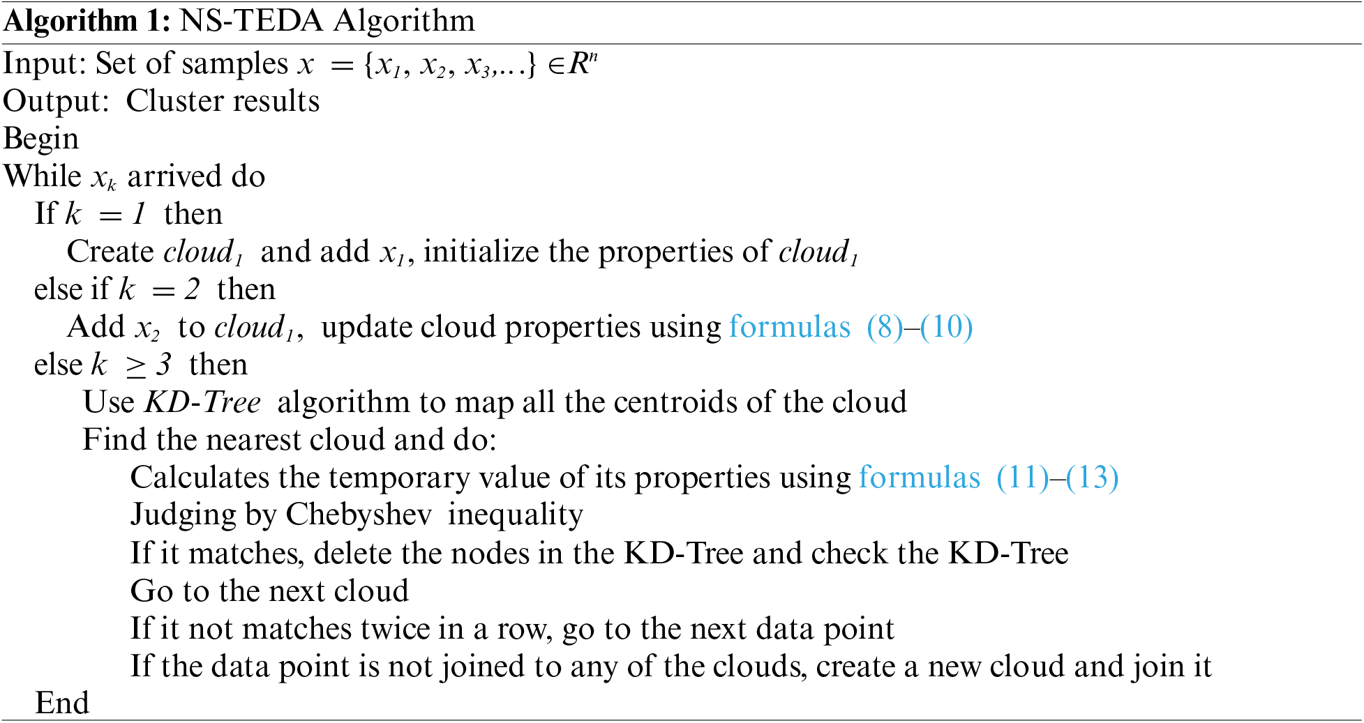
We combine the KD-Tree into the TEDA algorithm and name it the NS-TEDA (Neighbor Search based Typicality and Eccentricity Data analysis) algorithm, in the meantime, we have cited some of the Scapegoat Tree’s methods to make the two of them work better together. When the kth (k ≥ 3) data point enters, the centroids of all existing clouds are taken and constructed into a binary tree using the KD-Tree algorithm. While building the tree, we refer to the methods in the Scapegoat Tree to keep the KD-Tree balanced and record its imbalance α in each node of the KD-Tree, if the α of the current node is out of reasonable range, the uppermost node that needs to be reconstructed is found to perform a reconstruction operation to keep the KD-Tree balanced. The range of α is generally between 0.6 and 0.8, in our study, α takes the value of 0.75. The KD-Tree algorithm is then used to find the nearest neighbor of the current data point, and the data point is attempted to be placed into the cloud represented by the nearest neighbor, using Chebyshev inequality to make a determination. If it joins in that cloud, the node needs to be removed from the KD-Tree and checked if the KD-Tree needs to be reconstructed. If it does not satisfy Chebyshev’s inequality twice in a row, stop the operation and wait for the next data point to enter.

During the experimentation, we observed that the original TEDA algorithm requires traversing all existing clouds, while the algorithm combined with the KD-Tree only needs to operate on clouds that are closer in distance. Therefore, in the early stages of data stream arrival, when the number of existing clouds is low, the original TEDA algorithm may exhibit faster runtime. However, as the data stream gradually increases and the number of clouds grows, the combined algorithm’s runtime becomes faster. The combined algorithm typically operates on fewer than ten clouds, so the processing time for each newly arrived data point is approximately constant. As depicted in the line chart shown in Section 5, the combined algorithm’s runtime closely approximates a straight line, while the original TEDA algorithm may experience a rapid increase in runtime as the number of clouds grows with the influx of data points.

The flowchart and pseudocode of the NS-TEDA algorithm are shown in Fig. 1. After data xk is processed, all existing clouds need to be compared to all other clouds. The comparison conditions are as follows:

ski∩skj>ski−ski∩skj(15)

ski∩skj>skj−ski∩skj(16)

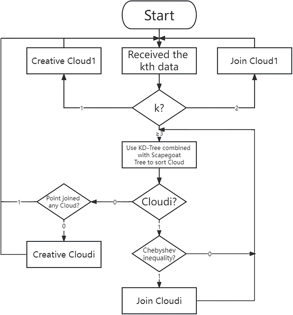
Figure 1: Flowchart of the NS-TEDA algorithm

If cloudi and cloudj meet the above conditions, cloudi and cloudj are combined. When the combination determination is completed, read the new data and continue the above operation.

5  Experiment and Discussion

In this section, we will illustrate the performance of the proposed algorithm through some comparative experimental illustrations and discuss the experimental results.

In order to verify the performance and efficiency of the combined model, in this section, the proposed algorithm is applied to some artificial datasets commonly used for data flow clustering and some real datasets of UCI.

5.1 Datasets

First of all, some data sets are taken from a specific data clustering library [32], which has been widely used in the validation of data clustering and has appeared in most data clustering studies. Each data set has been marked with some characteristics, and the specific information is shown in Table 1.

In Table 1, N represents the sample size of the data set, and K represents the number of categories of the data set.

5.2 Experiment Results

For the above datasets, the clustering results of the two-dimensional data set can be well shown by drawing. Next, this paper will show some results of the two-dimensional data set, from which we can intuitively see the quality of the clustering results.

Firstly, as can be seen from Table 1, A1, A2 data sets are composed of 3000 groups and 5250 groups of two-dimensional data, whose values are distributed in the range of 0 to 100000, and the clusters are basically spherical. The number of clusters of A1 and A2 is expected to be 20 and 35, respectively.

In Fig. 2, points of different colors represent the points belonging to different clusters, and the red pentagram in each cluster represents the position of the cluster center. S1 and S2 data sets are two-dimensional Gaussian clustering data sets with 5000 groups of different cluster overlaps, with cluster overlaps of 9% and 22%, respectively. The number of clusters of S1 and S2 is expected to be 15. The Unbalance dataset is an unbalanced dataset. In the actual case, the dataset is divided into eight clusters, where the three clusters on the left side of the data space contain 2000 data each, and the five clusters on the right side contain 100 clusters each.

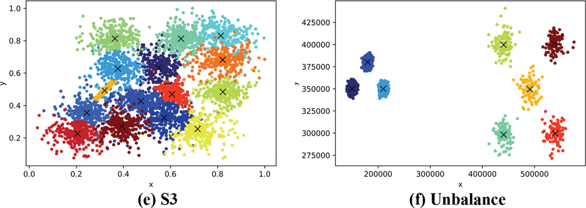
Figure 2: Clustering results for A1, A2, S1, S2, S3 and unbalance

The clustering results for data sets A1, A2, S1, S2, S3, and Unbalance are shown in Fig. 2. In Fig. 2, the blocks of different colors represent different clusters, and the X in the middle represent the central position of the cluster. The performance of the following dataflow clustering algorithm and the original TEDA algorithm against the improved TEDA algorithm is evaluated using a real dataset on UCI. The results of clustering are shown in Table 2. From Fig. 2, it can be observed that the combined algorithm yields favorable results in the aforementioned datasets. It can clearly separate them into multiple clusters, and the final number of clusters matches the expectations. The S3 dataset has a high degree of overlap, and we have tried several other data stream clustering algorithms, including the original TEDA algorithm, which cannot achieve satisfactory results on this dataset. Most algorithms tend to merge highly overlapping portions into the same cluster. However, when using the NS-TEDA algorithm, we can see that it produces better results. This is attributed to the NS-TEDA algorithm’s ability to prevent a data point from joining too many clouds to some extent, thereby reducing the likelihood of merging clusters with too many identical data points.

In Table 2, NMI, ARI, and Purity are the clustering evaluation indexes, all in the range of [0, 1], and the higher the value, the better. Table 2 shows that the original TEDA algorithm and the NS-TEDA algorithm work better on these data sets, and the NS-TEDA algorithm is similar to the original version. Next, we compare these two algorithms’ operational efficiency and stability separately. The results of the comparison between the original TEDA algorithm and the NS-TEDA algorithm are shown in Table 3.

From Table 3, it can be seen that after using the KD-Tree algorithm to optimize the TEDA algorithm, the adjustment of the parameter m needs to be changed to obtain the best clustering results. From the artificial data sets A1, A2, S1, S2, S3, and Unbalance, the range of m does not change much between the two algorithms in obtaining the optimal clustering results. Meanwhile, the TEDA algorithm did not achieve the same number of clusters as expected with the S3 dataset, and the final results always had two clusters merged due to higher overlap and closer distance, which was caused by the fact that most of the points in the neighboring locations of these two clusters joined both clusters at the same time. However, the NS-TEDA algorithm can obtain the same number of clusters as expected, which shows that the combination of the TEDA algorithm and KD-Tree algorithm can prevent the same data point from joining too many clusters to a certain extent, and reduce the situation that two different clusters are eventually merged when different clusters are close in space and have high overlap. The runtime comparison of Table 3 shows that the TEDA algorithm combined with the KD-Tree algorithm has a poorer runtime compared to the TEDA algorithm under the Iris, Wine, and Unbalance datasets because these datasets have a smaller amount of data and, within the dataset, are arranged by their accurate label. These datasets resemble continuous data. However, with other datasets with more extensive data volumes or datasets not arranged according to their accurate labels, the NS-TEDA algorithm can effectively reduce unnecessary operations when new data points are entered, thus improving its running efficiency.

Next, we will attempt to split the experiment to compare the performance of the algorithm. The speed of clustering for data sets A1, A2, S1, and S2 are shown in Fig. 3.

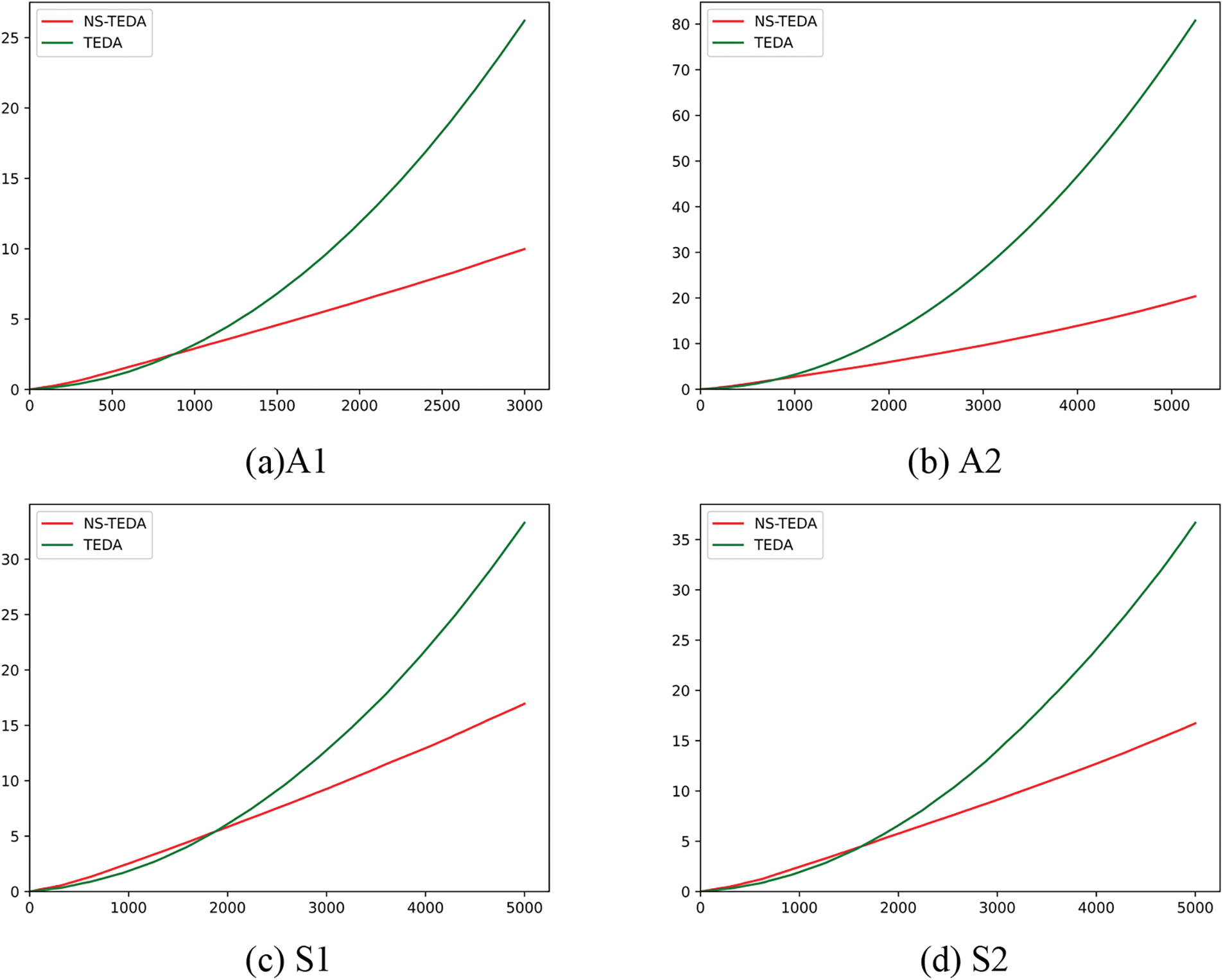
Figure 3: Runtime comparison using A1, A2, S1, S2

Fig. 3 compares the time required for NS-TEDA and TEDA algorithms to process newly entered data on the A1, A2, S1, and S2 datasets. From the graph, it can be seen that when there is less data, the TEDA algorithm has higher efficiency. However, as the data stream enters, the required running time of the NS-TEDA algorithm improves slowly. In the A-class dataset, the efficiency of NS-TEDA has already surpassed TEDA at around 500–1000, while in the S-class dataset, it is around 1500–2000, and the improvement is even more significant after that. In general, the Line chart of the time required for NS-TEDA to process data is closer to a straight line, while TEDA is closer to an exponential function curve.

Fig. 4 shows the NMI, ARI, and Purity indicators of the clustering results obtained by the NS-TEDA and TEDA algorithms on the iris and wine datasets with different parameters m. From the above figure, it can be seen that when the parameter selection is small, the result of the NS-TEDA algorithm has some slight fluctuation compared to the original TEDA algorithm, but it is not much different. However, as the parameter increases, the accuracy of the NS-TEDA algorithm is close to that of the TEDA algorithm, and it will be almost identical in the end. From Table 2, it can be seen that under reasonable parameters, the best clustering results of the two algorithms on the iris and wine datasets are not significantly different.

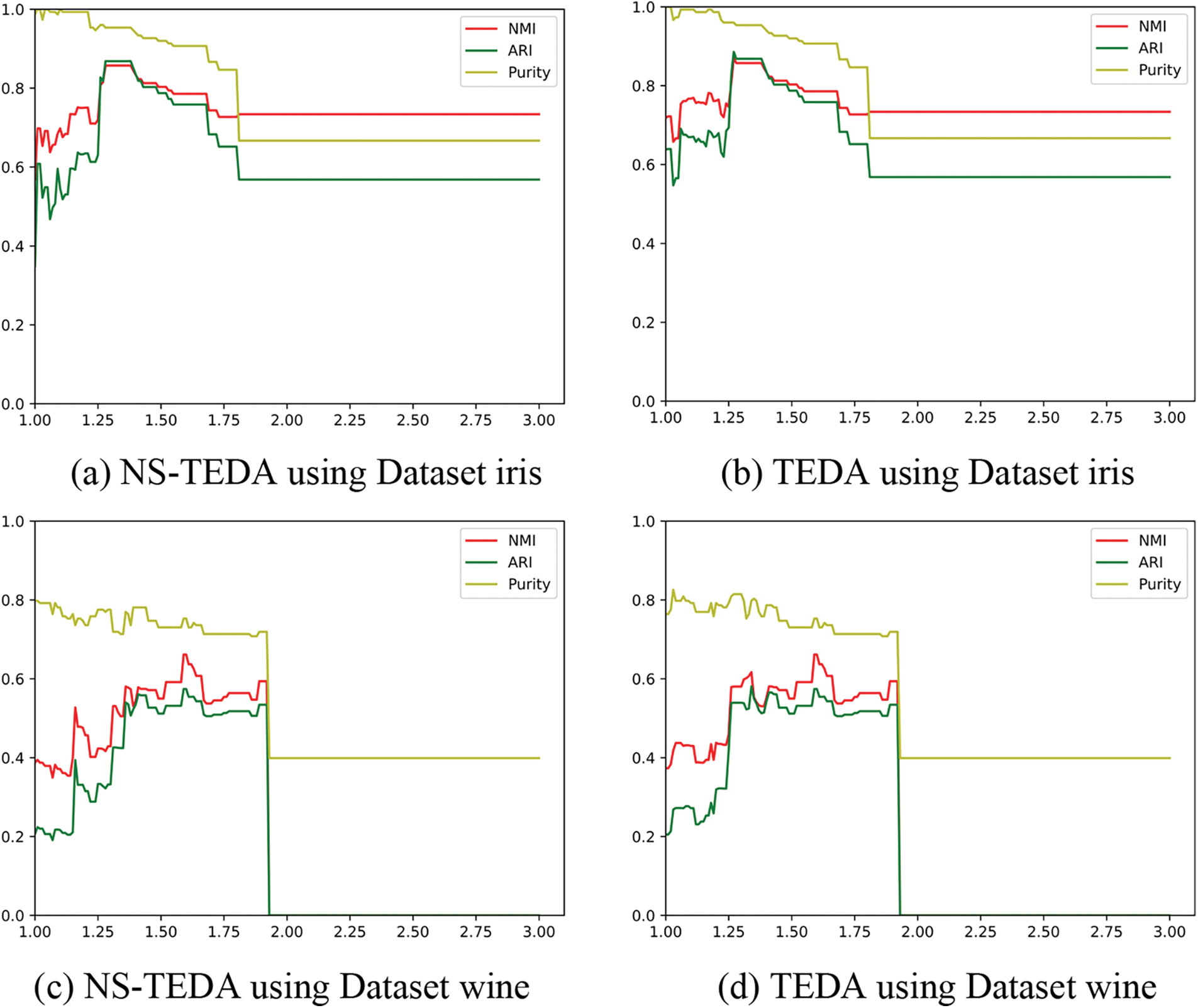
Figure 4: Comparison of clustering evaluation metrics using iris and wine

6  Conclusion

In this paper, we propose a novel algorithm called NS-TEDA, which combines the Optimized KD-Tree algorithm with the TEDA algorithm to perform clustering on online data streams. Our improved NS-TEDA algorithm inherits the advantages of the TEDA algorithm while incorporating the Optimized KD-Tree algorithm. When a new data point arrives, it only needs to interact with clusters close to the data point, reducing the computational burden associated with distant clusters. This enhances the algorithm’s efficiency while reducing the likelihood of excessive cluster assignments to the same data point, which could result in the merging of closely located clusters. Through the comparison of experimental results, we can observe that the accuracy of the NS-TEDA algorithm is superior to the original TEDA algorithm and some other data stream clustering algorithms in most cases. Moreover, the NS-TEDA algorithm exhibits significantly lower runtime on large datasets compared to the original TEDA algorithm, making it more suitable for clustering analysis in data streams. In practical applications of data stream clustering, such as network traffic analysis, sensor data analysis, real-time health monitoring, and more, the generated data is vast and continuously arriving. Clustering analysis for these data demands not only high accuracy but also efficient algorithms that can quickly present results as new data arrives. This requirement aligns well with the advantages of NS-TEDA.

NS-TEDA also has certain limitations. The NS-TEDA and TEDA algorithms typically utilize a parameter, denoted as “m”, which is commonly set to 3. However, in practical usage, adjusting the value of “m” is often necessary to achieve the best clustering results, this is not very convenient. In the combination of the TEDA algorithm and the KD-Tree algorithm, we determine whether we need to continue to operate on a data point by two consecutive occurrences of the data point being unsuitable for joining the cloud, which is not necessarily the optimal solution.

In future work, we intend to investigate an adaptive approach for determining the optimal value of “m”, enabling the algorithm to directly obtain the best clustering results without requiring manual adjustment and for the combination of the two algorithms in the combination of the two algorithms, an adaptive strategy is proposed to solve the problem of how to abort the operation of the data points on the cloud to make the combination of the TEDA algorithm and the KD-Tree algorithm more appropriate. Overall, the NS-TEDA algorithm offers a promising solution for clustering online data streams, combining efficiency and accuracy.

Acknowledgement: The authors would like to thank the editors and reviewers for their professional guidance, as well as the family and team members for their unwavering support.

Funding Statement: This research was funded by the National Natural Science Foundation of China (Grant No. 72001190) and by the Ministry of Education’s Humanities and Social Science Project via the China Ministry of Education (Grant No. 20YJC630173) and by Zhejiang A&F University (Grant No. 2022LFR062).

Author Contributions: Conceptualization, D.Y. Xu and J.M. Lü; methodology, J.M. Lü; software, J.M. Lü; validation, D.Y. Xu and X.Y. Zhang; formal analysis, H.T. Zhang; investigation, H.T. Zhang and D.Y. Xu; resources, D.Y. Xu; data curation, J.M. Lü; writing—original draft preparation, J.M. Lü and D.Y. Xu; writing—review and editing, X.Y. Zhang and H.T. Zhang; visualization, H.T. Zhang; supervision, H.T. Zhang; project administration, D.Y. Xu; funding acquisition, D.Y. Xu. All authors have read and agreed to the published version of the manuscript.

Availability of Data and Materials: The data that support the findings of this study are available from the corresponding author upon reasonable request.

Conflicts of Interest: The authors declare that they have no conflicts of interest to report regarding the present study.

References

1. P. Angelov, “Anomaly detection based on eccentricity analysis,” in 2014 IEEE Symp. Evol. Auton. Learn. Syst. (EALS), Orlando, FL, USA, 2014, pp. 1–8. [Google Scholar]

2. L. O’callaghan, N. Mishra, A. Meyerson, S. Guha, and R. Motwani, “Streaming-data algorithms for high-quality clustering,” in Proc. 18th Int. Conf. Data Eng., San Jose, CA, USA, 2002, pp. 685–694. [Google Scholar]

3. C. C. Aggarwal, S. Y. Philip, J. Han, and J. Wang, “A framework for clustering evolving data streams,” in Proc. 2003 VLDB Conf., Berlin, Germany, 2003, pp. 81–92. [Google Scholar]

4. R. Li, C. Wang, F. Liao, and H. Zhu, “RCD+: A partitioning method for data streams based on multiple queries,” IEEE Access, vol. 8, pp. 52517–52527, 2020. doi: 10.1109/ACCESS.2020.2980554. [Google Scholar] [CrossRef]

5. A. Liu, J. Lu, and G. Zhang, “Concept drift detection via equal intensity k-means space partitioning,” IEEE Trans. Cybern., vol. 51, no. 6, pp. 3198–3211, 2020. doi: 10.1109/TCYB.2020.2983962. [Google Scholar] [PubMed] [CrossRef]

6. Y. Alotaibi, “A new meta-heuristics data clustering algorithm based on tabu search and adaptive search memory,” Symmetry, vol. 14, no. 3, pp. 623, 2022. doi: 10.3390/sym14030623. [Google Scholar] [CrossRef]

7. T. Zhang, R. Ramakrishnan, and M. Livny, “BIRCH: An efficient data clustering method for very large databases,” ACM Sigmod Rec., vol. 25, no. 2, pp. 103–114, 1996. doi: 10.1145/235968.233324. [Google Scholar] [CrossRef]

8. Y. Cheung and Y. Zhang, “Fast and accurate hierarchical clustering based on growing multilayer topology training,” IEEE Trans. Neur. Netw. Learn. Syst., vol. 30, no. 3, pp. 876–890, 2018. doi: 10.1109/TNNLS.2018.2853407. [Google Scholar] [PubMed] [CrossRef]

9. J. W. Sangma, M. Sarkar, V. Pal, A. Agrawal, and Yogita, “Hierarchical clustering for multiple nominal data streams with evolving behaviour,” Complex Intell. Syst., vol. 8, no. 2, pp. 1737–1761, 2022. doi: 10.1007/s40747-021-00634-0. [Google Scholar] [CrossRef]

10. S. Nikpour and S. Asadi, “A dynamic hierarchical incremental learning-based supervised clustering for data stream with considering concept drift,” J. Amb. Intell. Humaniz. Comput., vol. 13, no. 6, pp. 2983–3003, 2022. doi: 10.1007/s12652-021-03673-0. [Google Scholar] [CrossRef]

11. F. Cao, M. Estert, W. Qian, and A. Zhou, “Density-based clustering over an evolving data stream with noise,” in Proc. of the 2006 SIAM Int. Conf. Data Min., Bethesda, MD, USA, 2006, pp. 328–339. [Google Scholar]

12. A. Amini, H. Saboohi, T. Herawan, and T. Y. Wah, “MuDi-stream: A multi density clustering algorithm for evolving data stream,” J. Netw. Comput. Appl., vol. 59, pp. 370–385, 2016. doi: 10.1016/j.jnca.2014.11.007. [Google Scholar] [CrossRef]

13. S. Laohakiat, S. Phimoltares, and C. Lursinsap, “A clustering algorithm for stream data with LDA-based unsupervised localized dimension reduction,” Inf. Sci., vol. 381, pp. 104–123, 2017. doi: 10.1016/j.ins.2016.11.018. [Google Scholar] [CrossRef]

14. M. K. Islam, M. M. Ahmed, and K. Z. Zamli, “A buffer-based online clustering for evolving data stream,” Inf. Sci., vol. 489, pp. 113–135, 2019. doi: 10.1016/j.ins.2019.03.022. [Google Scholar] [CrossRef]

15. A. Faroughi, R. Boostani, H. Tajalizadeh, and R. Javidan, “ARD-stream: An adaptive radius density-based stream clustering,” Future Gener. Comput. Syst., vol. 149, pp. 416–431, 2023. doi: 10.1016/j.future.2023.07.027. [Google Scholar] [CrossRef]

16. I. Ntoutsi, A. Zimek, T. Palpanas, P. Kröger, and H. P. Kriegel, “Density-based projected clustering over high dimensional data streams,” in Proc. 2012 SIAM Int. Conf. Data Min., Anaheim, CA, USA, 2012, pp. 987–998. [Google Scholar]

17. V. Bhatnagar, S. Kaur, and S. Chakravarthy, “Clustering data streams using grid-based synopsis,” Knowl. Inf. Syst., vol. 41, pp. 127–152, 2014. doi: 10.1007/s10115-013-0659-1. [Google Scholar] [CrossRef]

18. J. Chen, X. Lin, Q. Xuan, and Y. Xiang, “FGCH: A fast and grid based clustering algorithm for hybrid data stream,” Appl. Intell., vol. 49, pp. 1228–1244, 2019. doi: 10.1007/s10489-018-1324-x. [Google Scholar] [CrossRef]

19. M. Tareq, E. A. Sundararajan, M. Mohd, and N. S. Sani, “Online clustering of evolving data streams using a density grid-based method,” IEEE Access, vol. 8, pp. 166472–166490, 2020. doi: 10.1109/ACCESS.2020.3021684. [Google Scholar] [CrossRef]

20. S. Hu et al., “An enhanced version of MDDB-GC algorithm: Multi-density DBSCAN based on grid and contribution for data stream,” Process., vol. 11, no. 4, pp. 1240, 2023. doi: 10.3390/pr11041240. [Google Scholar] [CrossRef]

21. M. S. Yang, C. Y. Lai, and C. Y. Lin, “A robust EM clustering algorithm for Gaussian mixture models,” Pattern Recognit., vol. 45, no. 11, pp. 3950–3961, 2012. doi: 10.1016/j.patcog.2012.04.031. [Google Scholar] [CrossRef]

22. M. Ghesmoune, M. Lebbah, and H. Azzag, “A new growing neural gas for clustering data streams,” Neural Netw., vol. 78, pp. 36–50, 2016. doi: 10.1016/j.neunet.2016.02.003. [Google Scholar] [PubMed] [CrossRef]

23. N. Wattanakitrungroj, S. Maneeroj, and C. Lursinsap, “BEstream: Batch capturing with elliptic function for one-pass data stream clustering,” Data Knowl. Eng., vol. 117, pp. 53–70, 2018. doi: 10.1016/j.datak.2018.07.002. [Google Scholar] [CrossRef]

24. T. T. Nguyen, M. T. Dang, A. V. Luong, A. W. C. Liew, T. Liang, and J. McCall, “Multi-label classification via incremental clustering on an evolving data stream,” Pattern Recognit., vol. 95, pp. 96–113, 2019. doi: 10.1016/j.patcog.2019.06.001. [Google Scholar] [CrossRef]

25. D. Kangin, P. Angelov, and J. A. Iglesias, “Autonomously evolving classifier TEDAClass,” Inf. Sci., vol. 366, pp. 1–11, 2016. doi: 10.1016/j.ins.2016.05.012. [Google Scholar] [CrossRef]

26. P. Angelov, “Typicality distribution function—A new density-based data analytics tool,” in 2015 Int. Joint Conf. Neural Netw. (IJCNN), IEEE, 2015, pp. 1–8. [Google Scholar]

27. J. G. Saw, M. C. K. Yang, and T. C. Mo, “Chebyshev inequality with estimated mean and variance,” Am. Stat., vol. 38, no. 2, pp. 130–132, 1984. [Google Scholar]

28. J. Maia et al., “Evolving clustering algorithm based on mixture of typicalities for stream data mining,” Future Gener. Comput. Syst., vol. 106, pp. 672–684, 2020. doi: 10.1016/j.future.2020.01.017. [Google Scholar] [CrossRef]

29. J. L. Bentley, “Multidimensional binary search trees used for associative searching,” Commun. Acm., vol. 18, no. 9, pp. 509–517, 1975. doi: 10.1145/361002.361007. [Google Scholar] [CrossRef]

30. S. M. Omohundro, Five Balltree Construction Algorithms. Berkeley: International Computer Science Institute, pp. 1–22, 1989. [Google Scholar]

31. M. S. Charikar, “Similarity estimation techniques from rounding algorithms,” in Proc. Thiry-Fourth Annu. ACM Symp. Theory Comput., New York, NY, USA, 2002, pp. 380–388. [Google Scholar]

32. S. I. Boushaki, N. Kamel, and O. Bendjeghaba, “A new quantum chaotic cuckoo search algorithm for data clustering,” Expert Syst. Appl., vol. 96, pp. 358–372, 2018. doi: 10.1016/j.eswa.2017.12.001. [Google Scholar] [CrossRef]