MSADCN: Multi-Scale Attentional Densely Connected Network for Automated Bone Age Assessment

1  Introduction

Bone Age (BA) is the age of the human skeleton, which is different from a person’s actual age. BA is inferred from the skeleton’s growth, maturation, and aging patterns [1], and bone age assessment (BAA) is a medical diagnostic procedure. By analyzing X-rays of the left hand, medical specialists predict a patient’s skeletal age and compare it with the patient’s actual age, then determine whether the growth rate and bone maturation are regular. It is a diagnostic and therapeutic guide for adolescent growth and development abnormalities, hereditary diseases and chronic diseases [1–3]. BAA is widely used in pediatric clinical, sports medicine, forensic medicine, and genetic medicine [2,3].

In clinical medicine, Greulich-Pyle (G-P) [4] and Tanner-Whitehouse (TW3) [5] are the most common BAA methods. The G-P method establishes two sets of standard templates for males and females and derives bone age estimates by comparing the subject’s radiographs to gender-specific profiles. The G-P method is primary and quick, but it is subjective and image comparisons cannot be performed with absolute precision. The TW3 method divides a hand bone into 20 regions of interest (ROI) and derives bone age by comprehensively analyzing each ROI. Compared to the G-P method, TW3 can reduce the impact of subjective and individual differences and can improve the prediction accuracy. However, it is complex and time-consuming in clinical practice.

In addition, machine learning techniques-based methods have provided various analysis for medical image processing, especially automatic BAA. Generally, traditional automatic BAA methods extract manually labeled features, classify them by linear or nonlinear filters, and then map the categories to BA [6–9]. However, manually extracted features require high expertise for the marker.

In recent years, deep learning-based methods have focused on locating critical regions using bounding boxes and critical point annotations. Then, the labeled data is fed into the CNN to learn and extract the appropriate features [10–13]. However, manual annotation and specialized domain knowledge are inapplicable in large-scale application scenarios. Besides, most existing BAA systems primarily rely on CNN structures. They build deep convolutional neural networks (DCNNs) by simply stacking convolutional layers, which impede gradient propagation and are prone to gradient disappearance [14]. Several solutions to this problem have been proposed in related papers, including residual networks (ResNet) [15], fractalNets [16] and high-speed neural networks [17]. However, these methods are not applicable for limited training data, particularly for medical image processing. To address these issues and develop a reliable and automatic BAA method, we propose the multi-scale attentional densely connected network (MSADCN). The advantages of this network include:

1.    A new multi-scale convolutional structure is designed to extract rich and complementary information from hand bone images. The multi-scale convolutional layers are densely connected into dense blocks, which can make the feature information efficiently transmitted.

2.    Within the densely connected blocks, the coordinate attention mechanism (CAM) is embedded, which directs the network to focus on more helpful information and automatically locate the ROI of the most distinguished hand bones.

3.    Transfer learning is applied to train the proposed MSADCN on the public dataset IMDB-WIKI, and the obtained pre-training weights are loaded onto the RSNA dataset. Besides, label distribution learning and expectation regression are implemented to get the bone age expectation. Experimental evaluations show that the performance of MSADCN outperforms some mainstream neural network methods.

2  Related Work

In previous clinical BAA tasks, G-P and TW3 methods were time-consuming, error-prone and subjective. Therefore, scholars have been exploring the use of computer-aided medical image processing and analysis to design automated BAA methods. These methods can be divided into traditional and deep learning-based BAA methods. This section will briefly introduce the representative studies of both.

2.1 Traditional BAA Methods

Most traditional image processing BAA methods mainly have three steps. Firstly, extract manually designed features from an entire image or a specific ROI. Then, classify these features with a classifier trained with a few samples. Finally, the BAA results are obtained by matching the classification results with the corresponding classes. Niemeijer et al. [6] developed a automatic BAA method. They segmented bone blocks by using an active shape model technique to obtain shape and texture information of hand bones. de Luis-Garcia et al. [7] segmented ROI by active contours (SNAKES) to determine the outlines of bone blocks. Pan et al. [8] extracted bone features by segmenting images of the wrist using Gradient Vector Flow (GVF) combined with SNAKES. Giordano et al. [9] designed a fully automated BAA system, which extracted epiphyseal and metaphyseal ROIs (EMROIs) using image processing techniques. Then, it extracted the corresponding bone block characteristics by the TW2 criterion. Thodberg et al. [18] created a three-layer architecture called Bone Xpert, including a bone reconstruction model, feature analysis and bone age prediction. Kashif et al. [19] proposed the scale-invariant feature transform (SIFT) to extract critical features at specific locations of bone blocks, and then classify them using SVM to get bone age assessment. Due to these methods based on manual extraction of hand bone feature regions, they obtained limited performance with the MAE results ranging from 10 to 28 months. The BAA methods based on traditional techniques require manual extraction of specific features, which need a high level of expertise for the marker and cannot compete with medical experts.

2.2 Deep Learning-Based BAA Methods

Nowadays, deep learning-based methods have been essential in medical image processing [20–22], which can learn the intrinsic structures and patterns of the input data through specific algorithms. Accordingly, a variety of deep learning methods for BAA have been presented, some of which exceed the performance of experts. Lee et al. [23] utilized pre-trained fine-tuned CNN for BAA, which obtained 57.32% and 61.40% accuracy for females and males, respectively. Spampinato et al. [10] designed BoNet for BAA by using a deformation layer to address bone non-rigid deformation. Liu et al. [11] developed a multi-scale data fusion framework based on non-subsampled contour wave transform (NSCT) and CNN to acquire multi-scale and multi-directional features. Li et al. [12] designed a CNN for fine-grained bone age image classification. This network can automatically locate ROI and fuse the extracted local features with the global features, which get the accuracy for males and females with 66.38% and 68.63%, respectively. Nguyen et al. [13] extracted the hand key points by pre-processing images. They applied transfer learning to gender determination and the BAA model, which obtained an MAE of 5.31 months. Deng et al. [24] manually segmented the articular surfaces and epiphyseal ROIs of hand bones, and then used five mainstream CNNs to predict bone age. Li et al. [25] used visual heatmaps to locate the epiphyseal region and combined gender input into the bone age prediction network. Jian et al. [26] developed a multi-feature lateral fusion TENet,which extracted ROIs using hand topology blocks while enhancing hand bone edge features.

In recent years, many studies have applied attentional localization to the ROI of the input images. Fu et al. [27] devised an RA-CNN algorithm, which iteratively generates region attention by recursively learning multi-scale and fine-grained feature maps. Chen et al. [28] obtained attention maps of the hand bone by training a classification network to obtain the critical regions and aggregating them from different detected regions. Zulkifley et al. [29] proposed an attention-aware network (AXNet) to normalize hand bone images and predict bone age. Ren et al. [30] proposed a weakly supervised regression CNN by using an attention module to generate coarse and fine attention maps, which obtained the MAE between 5.2 and 5.3 months. Deep learning-based BAA methods automatically extract ROIs through CNN and predict bone age by using classification or regression ideas, which can save time, be robust, and provide more accurate results.

3  Methods

In this paper, the BAA task is divided into three modules: (1) image pre-processing, (2) MSADCN-based feature extraction phase, and (3) regression of bone age expectation based on label distribution learning. Fig. 1 depicts the proposed method of the BAA task. Firstly, the input X-rays are pre-processed to get high-resolution and low-noise images of the same size. Then, MSADCN is loaded with pre-trained weights on the IMDB-WIKI dataset, and transfer learning is used to extract features and automatically locate ROIs from the processed hand bone images. Finally, the extracted features are combined with the gender information of each image to obtain the bone age estimates through labeled segment learning. The three modules will be introduced in detail as follows.

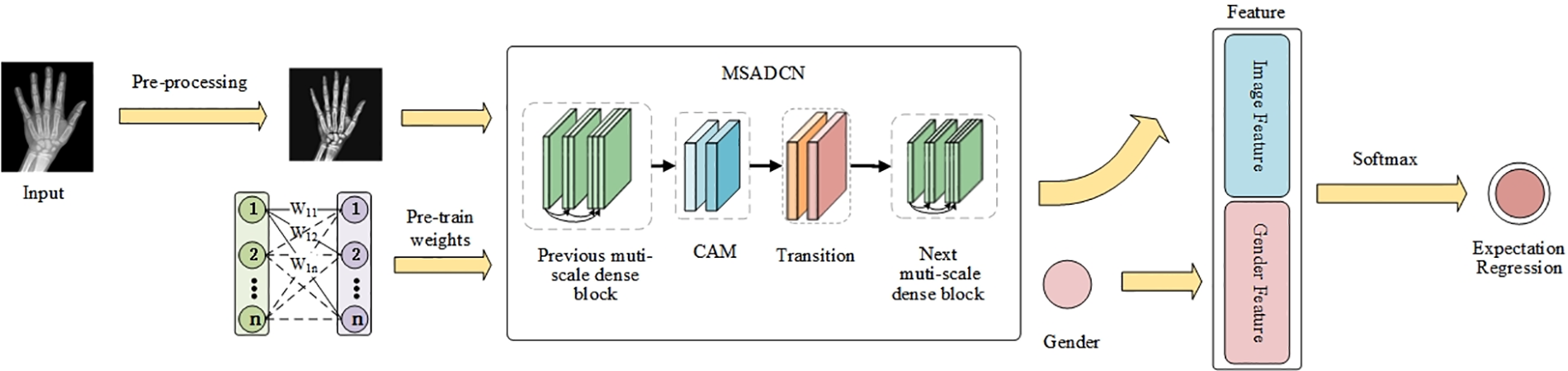
Figure 1: The proposed framework of MSADCN for the BAA task

3.1 Image Dataset and Preprocessing

The RSNA dataset has 14236 hand radiographs, including 12611 training images, 1425 validation images, and 200 test images. Since the RSNA dataset are from different hospitals, the hand bone images have different sizes, high resolution, and noise. Therefore, to get more accurate image training results, the training images used in this paper refer to the image segmentation technique [31]. Fig. 2a shows the image before segmentation, while Fig. 2b is the segmented image with a resolution of 1600 × 2080 pixels.

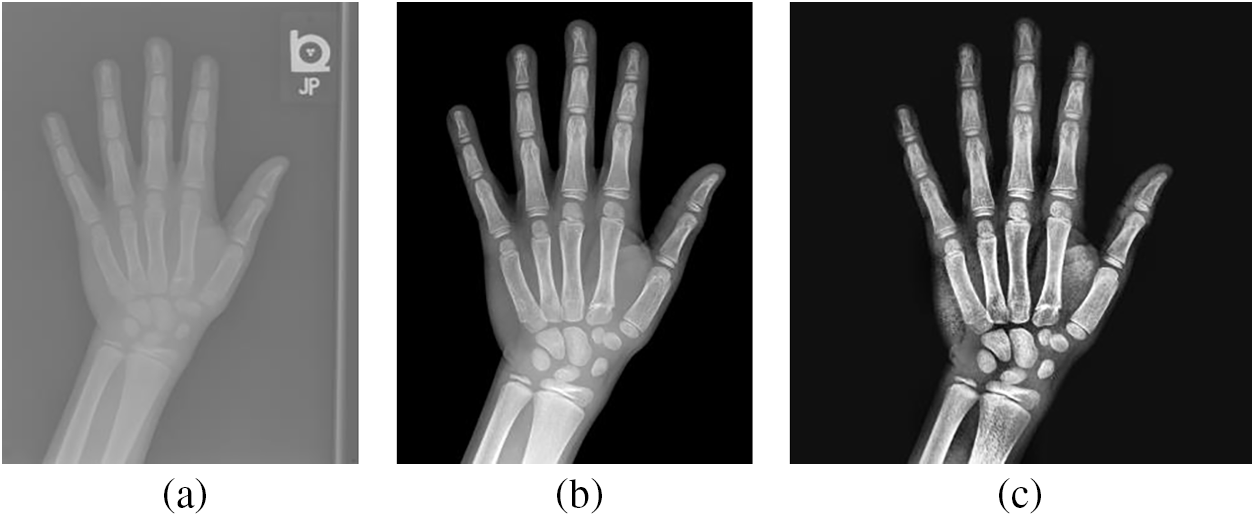
Figure 2: Comparison of hand bone images: (a) The original X-rays; (b) The segmented X-rays; (c) The pre-processed X-rays

To get the more distinct area of the hand bone, the segmented image is preprocessed. First, the appropriate size of the image is obtained by cropping the image borders and adjusting the width and height ratios. Then, the image is scaled using bi-trivial interpolation in a 4 × 4 pixels region, and histogram equalization is utilized to enhance the image contrast. Finally, to ensure the consistency of input data, the preprocessed image size is 512 × 512 pixels in Fig. 2c.

3.2 MSADCN-Based Feature Extraction Phase

The MSADCN-based feature extraction process will be described in this section. Firstly, the composition of the multi-scale dense connectivity mechanism is introduced, which consists of multi-scale dense blocks, CAM, and transition layer. Secondly, two-component structures are highlighted: the multi-scale module for extracting multi-scale features and the coordinate attention module for focusing on essential features. Finally, we will introduce the pre-training method on the IMDB-WIKI dataset. Next, each component is described in detail.

3.2.1 Multi-Scale Dense Connection Mechanism of MSADCN

The multi-scale dense connection mechanism of MSADCN based on the principle that each layer receives feature information from all former layers in the channel direction. Then the feature maps received by the Lth layer can be expressed as a nonlinear function:

XL=HL([X0,X1,⋅⋅⋅,XL−1])(1)

where [X0,X1,⋅⋅⋅,XL−1] denotes the feature maps connection from layer 0th to layer L-1th. HL(⋅) represents the nonlinear transformation of layer L, which includes batch normalization (BN), rectified linear unit (ReLU) and the multi-scale 3 × 3 convolution (Conv) kernel. To decrease the amount of input feature maps during the information transfer process and improve the computational efficiency, we insert 1 × 1 Conv before the multi-scale 3 × 3 Conv. Therefore, as shown in Fig. 3a, the nonlinear function HL(⋅) of the multi-scale dense layer consists of BN, ReLU, 1 × 1 Conv, and multi-scale 3 × 3 Conv. In Fig. 3a, the growth rate k is 3, which can generate 4k feature maps following a 1 × 1 Conv. Accordingly, a dense connection of multiple dense layers forms a multi-scale dense block. Fig. 3b shows a dense block with three multi-scale dense layers. Since each multi-scale dense layer produces only k feature maps, the number of feature maps generated by the Lth layer can be expressed as follows:

NL=k0+k×(L−1)(2)

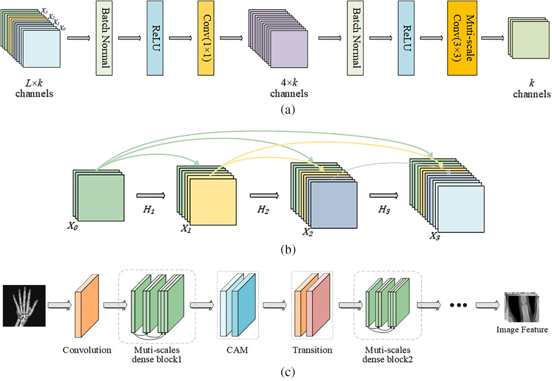
Figure 3: The general structure of MSADCN: (a) Multi-scale dense layer; (b) Multi-scale dense block; (c) MSADCN for feature extraction of hand bone images

where k0 denotes the number of output image channels. In addition, there is a transition layer between each multi-scale dense block to downsample and compress the model. Assuming that the number of output channels from the previous layer is m, the size of features is θm after the transition layer, where θ is the compression factor, 0<θ≤1. Fig. 3c shows the structure of the feature extraction network MSADCN, which consists of two multi-scale dense blocks, CAM and transition layer.

3.2.2 Multi-Scale Module

Inspired by Res2Net, which can enhance the capability of multi-scale representation at a finer granularity level [32], we propose an efficient method for creating convolutional modules with gradually increasing scales in a single convolutional module. The multi-scale module is one of the essential structures of MSADCN, which can obtain more accurate feature maps during the feature extraction phase of the BAA task. Next, the multi-scale module will be described in detail.

Fig. 4 depicts the structure of the multi-scale module, which is the constitutive principle of the multi-scale 3 × 3 Conv in the dense layer in Fig. 3a. We assume that the 4k input feature maps from all prior layers are rearranged and divided into s groups. Each group has 4k/s feature maps from different dense layers. Since the number of produced feature maps increases with the depth of multi-scale dense blocks, we directly connect the 1 × 1 Conv to the first group of the permutation operation, and the other groups employ 3 × 3 Conv with regularization processing and activation function before convolution. To reduce the number of parameters, we design the output channel of each 3 × 3 Conv as 4k/s. After finishing all 3 × 3 Conv operations, the first group without convolution is spliced after the output feature maps of all 3 × 3 Conv. Finally, the features at different scales are fused by 1 × 1 Conv. Significantly, the number of output channels at this stage equals the input channels. To maintain the characteristic that each multi-scale dense layer produces only feature maps in the dense connection mechanism, the output channels after 1 × 1 Conv are set to be the same as the growth rate, then as the input to the next layer.

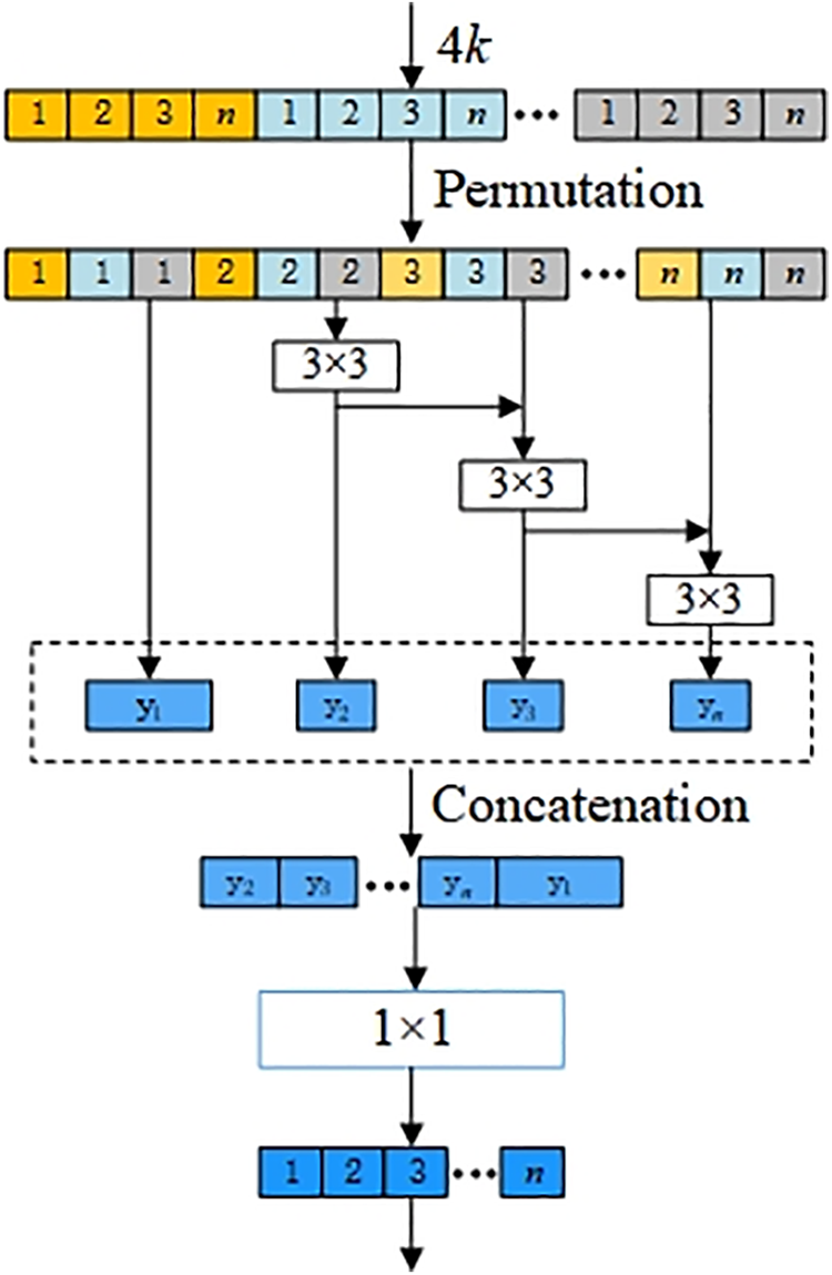
Figure 4: Multi-scale structure of dense layer in MSADCN

Next, we will analyze the number of parameters generated by the multi-scale dense layer convolution structure of MSADCN and compare it with DenseNet [33]. The input and output channels of the dense layer are the same in DenseNet and MSADCN, respectively.

In a dense layer of DenseNet, the number of input feature maps for 1 × 1 Conv is lk, and output feature maps after 1 × 1 Conv are 4k. The number of input and output feature maps for 3 × 3 Conv are 4k and k, respectively. Therefore, the number of parameters after a dense layer in the DenseNet structure can be expressed as follows:

PDenseNet=lk×4k+4k×k×3×3=4lk2+36k2(3)

In Fig. 4, the first group (the first 4k/s feature maps) has no parameters in the convolution layer, while the input and output channels of the first 3 × 3 Conv are 4 k/s. The input channels of other 3 × 3 Conv are 8 k/s, and its number of output channels is 4k/s. Since the outputs of the first group and all 3 × 3 Conv groups are the inputs of 1 × 1 Conv, it generates k output channels after the 1 × 1 layer. Consequently, the total number of parameters of a multi-scale dense layer in MSADCN can be summarized as follows:

PMSADCN=lk×4k+4ks×4ks×3×3+8ks×4ks×3×3×(s−2)+[4ks+(s−1)×4ks]×k=4lk2+(288s−432s2+4)×k2(4)

By comparing PDenseNet and PMSADC, it can be seen that both have a similar number of parameters (the value of growth rate k is set to 32, and s is set to 8). Although the multi-scale module makes the convolution process of MSADCN somewhat more complicated than DenseNet, the number of parameters is not multiplied (within an acceptable range), and the information transmission of MSADCN feature maps is superior to DenseNet. Additionally, several convolution kernels perceive the information better than a convolution kernel, which can extract more accurate feature information. Therefore, MSADCN can effectively capture the information from multiple scales in the source images and achieve good results for the BAA task.

3.2.3 The Coordinate Attention Module

Due to the vital feature reuse of the multi-scale dense connectivity mechanism, the MSADCN generates a certain number of feature maps during the propagation process. To make the feature transfer between dense layers more effective, the coordinate attention mechanism (CAM) [34] is embedded after the multi-scale dense block. CAM can redistribute the raw features extracted by MSADCN, and the model’s learning ability can be enhanced by focusing on essential features and suppressing unnecessary features. Next, the structure of the attention module is described in detail.

CAM can be seen as a computing unit for enhancing the feature representation of a neural network, which accepts intermediate feature X=[x1,x2,⋯,xc]∈RC×H×W as input and produces augmented feature Y=[y1,y2,⋯,yc] of the same size. Fig. 5 illustrates CAM encodes channel and long-distance relations of two processes: coordinate information embedding (CIE) and coordinate attention generation (CAG).

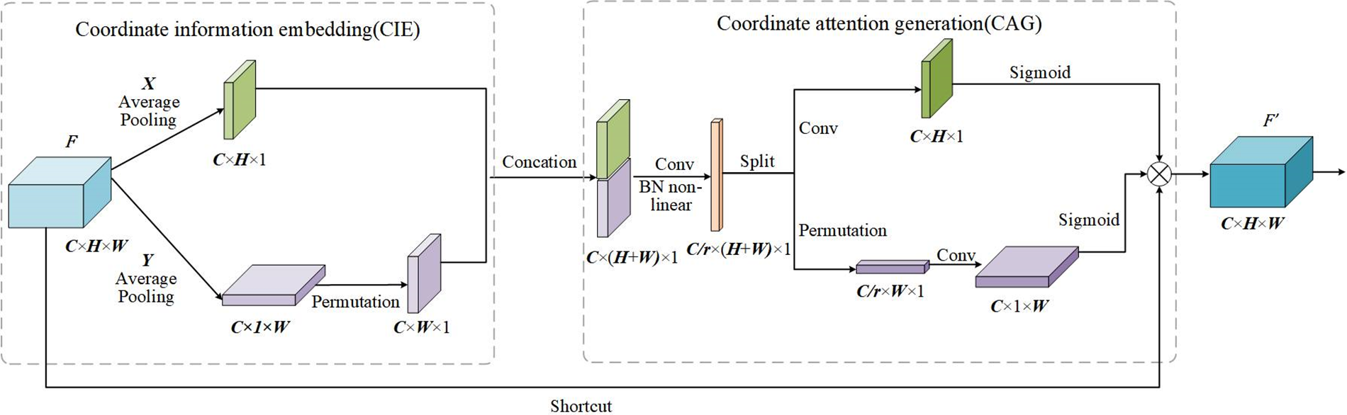
Figure 5: The execution process of CAM

In the CIE phase, CAM uses two pooling kernels (H,1) and (1,W) to encode spatial information, which obtains the feature of dimension C × 1 × W and C × H × 1, respectively. Therefore, the output of the cth channel with width w can be expressed as

zch(w)=1W∑0≤j<Hxc(j,w)(5)

where xc(j,w) denotes the value of feature maps. Similarly, given a height of h, the output of the cth channel can be expressed as

zch(h)=1W∑0≤i<Wxc(h,i)(6)

Eqs. (5) and (6) enable the attention block to acquire distant dependencies along one of the spatial directions while maintaining accurate location information along the other spatial direction, which can help our model to localize the ROI more accurately.

In the CAG phase, the features generated by Eqs. (5) and (6) are concatenated. Then, the features are transformed by the 1 × 1 Conv function, BatchNorm, and nonlinear activation as follows:

f=δ(F1([zh,zw]))(7)

where [zh,zw] denotes the concatenation operation of the spatial feature in Eqs. (5) and (6), δ is a nonlinear activation function, f∈RC/r×(H+W) is an intermediate feature, and r is a reduction factor. Then, f is divided into two features, fh∈RC/r×H and fw∈RC/r×W, which are transformed into a tensor by two 1 × 1 Conv (Fh and Fw) with the same channels as the input X. After that, the feature transformation is performed by a sigmoid function σ to make its dimension consistent with the input X. These processes can be expressed as follows:

gh=σ(Fh(fh))(8)

gw=σ(Fw(fw))(9)

Finally, to create a new feature map by integrating all the sub-feature maps, outputs gh and gw are ultimately integrated into a weight matrix as follows:

yc(i,j)=xc(i,j)×gch(i)×gcw(j)(10)

After the input feature maps are processed by CIE and CAG, the weights of each feature map comprise channels, horizontal spatial, and vertical spatial information. MSADCN has the nature of feature reuse, however, not every feature information needs to be utilized completely. Therefore, the CAM module is introduced to focus on the critical features of the network. CAM can generate more discriminative feature representations by rearranging the original feature maps and enhancing channel information exchange. In this paper, the CAM module was embedded between the previous dense block and the subsequent transition of the MSADCN. As shown in Fig. 6, the feature maps F∈RC×H×W generated from the previous multi-scale dense block input the CAM module, which can obtain the attention maps from the channel and position information. Then, the output feature maps F′∈RC×H×W are obtained by redistributing the original feature maps’ weights, which are input to the transition module, downsampled by the transition layer and ultimately input to the next dense block.

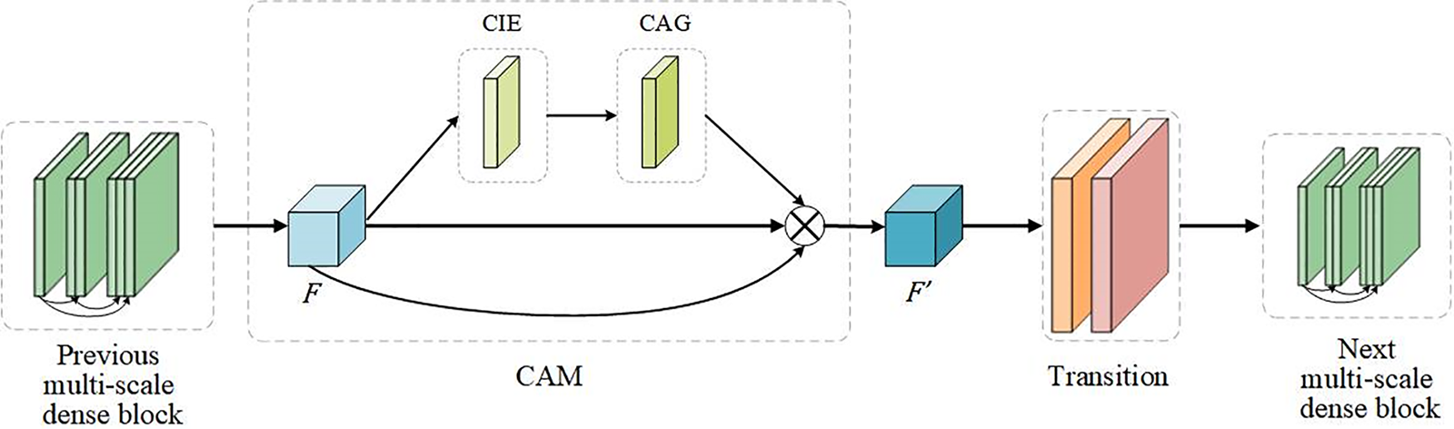
Figure 6: The attention module of MSADCN

3.2.4 The Pre-Training Method for the BAA Task

IMDB-WIKI is a large face dataset with over 500 thousand images, which can be used for age prediction, face recognition, and other tasks. To ensure the significant similarity between the face age prediction task and the target task of the bone age prediction, we first apply the same pre-processing to IMDB-WIKI. Then, input the pre-processed images and gender information into MSADCN for training to get the age prediction results. Finally, we use the trained model with the best face age prediction results as the pre-trained weights for the BAA task. The generalization ability of the MSADCN model is improved by model adaptation, which transfers the feature extraction capabilities learned in the face prediction domain to the bone age prediction domain.

3.3 Regression of Bone Age Expectation

In practical applications, radiographs look very similar if images are of similar age. For instance, when a person’s bone age is 280 or 281 months, their radiographs are almost identical. Existing methods view the BAA task as a general regression or a discrete classification problem and do not take full advantage of the correlation information between adjacent ages, which can affect the accuracy of bone age prediction. Therefore, we exploit the correlation of hand images in adjacent ages to learn the age distribution for each hand image instead of a single age label by using label distribution learning (LDL) [35,36]. This can prevent the network from overconfidence and yield more robust age estimates.

The age distribution includes a collection of probability values, illustrating how each age impacts the hand picture and depicts the connection between adjacent ages. We assume that F(xi)∈Rm is the feature information output from the feature extraction network MSADCN, G(gi)∈Rn is the gender information of the i th sample (−1 for female and 1 for male), where m and n denote the dimension of the image and gender features, respectively. Fig. 7 shows the LDL-based bone age prediction process. Firstly, the feature and gender information are fused by fi=[F(xi);G(gi)]∈Rm+n, which will be transmitted to a fully connected layer zi∈R240 as follows:

zi=WTfi+b(11)

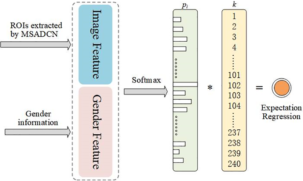
Figure 7: LDL-based bone age expectation regression

where WT is the weight matrix of features, and b is the bias. Then, converting zi into an age distribution by the activation function of Eq. (12).

pi,k=exp⁡(zi)∑kexp⁡(zi),k=1,2,⋅⋅⋅,240(12)

where pi,k denotes the probability that the i th sample belongs to age k, k∈{1,2,⋯,240}. Finally, the output layer obtains the expectation of bone age y^i.

y^i=∑k=1k=240k⋅pi,k(13)

For a given sample of input characteristics and gender information, the regression task aims to minimize the MAE, which reflects the error between the actual age y and the predicted age y^. The lower its value, the better the performance.

LMAE=1N∑i=1N|y^i−yi|(14)

A Gaussian distribution [37] Gi,k represents the probability of age k associated with the i th data. σ is the hyperparameter in charge of the age uncertainty.

Gi,k=12πσexp⁡{−(k−yi)22σ2}(15)

The predicted age distribution should be concentrated in a small range of the actual age and follow a Gaussian distribution. However, this property is difficult to guarantee. The estimated age distribution should be centred on a smaller range of actual ages and follow a Gaussian distribution. However, this property is difficult to guarantee. Therefore, two criterions are used in this paper to assess the merit of the training parameters. One criterion is MAE, and the other criterion is the similarity between the target probability and the predicted probability distribution, measured by Kullback-Leibler (KL) [38] scatter. The loss function KL can be described as follows:

LKL=1N∑i=1N∑k=1240pi,kln⁡pi,kGi,k(16)

where pi,k and Gi,k are described respectively in Eqs. (12) and (15). Finally, we use LMAE and LKL to define the joint loss function L.

L=λMAELMAE+λKLLKL(17)

where λMAE and λKL are the hyperparameters that balance the loss functions LMAE and LKL, respectively.

Besides, root mean square error (RMSE) is adopted as the evaluation metric, y and y^ denote the actual age and the predicted age, respectively.

RMSE=1N∑i=1N(y^i−yi)2(18)

4  Experiment Result and Analysis

The proposed model is trained on the Windows 10 operating system. The hardware environment is AMD Ryzen 75800H with Radeon Graphics @ 3.20 GHz processor, 16G RAM and NVIDIA GeForce RTX 3080Ti Laptop GPU. The software environment is Python 3.6, the deep learning framework is PyTorch, and the development tool is PyCharm 2021.

Since the RSNA dataset has 200 test images without published bone age, our model is tested on the RSNA test set, and obtains the bone age prediction result MAE of 4.64 months. Fig. 8 shows the relationship of actual age between deviation age and predicted age. We assume the deviation is the difference between predicted and actual age. As shown in Fig. 8a, the absolute deviation of the prediction result is stable within 15 months and is mainly concentrated within eight months. From Fig. 8b, we can see that our predicted age is highly consistent with the actual age for males and females, which demonstrates the proposed model can achieve excellent performance.

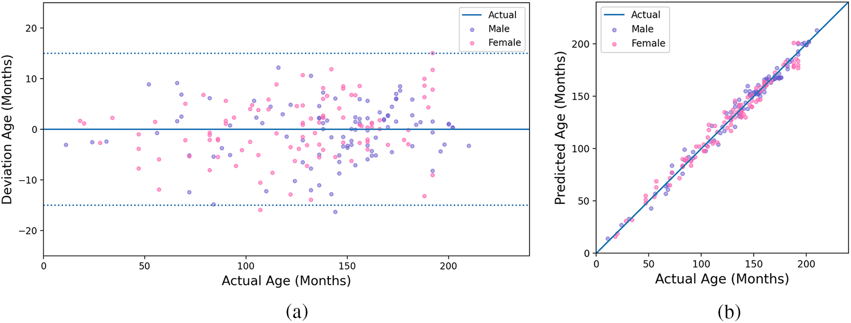
Figure 8: Experimental results of the proposed method. (a) The result of actual and deviation age; (b) The result of actual and predicted age

Fig. 9 is the loss comparison between the initial weights and the loaded pre-trained weights of MSADCN. Fig. 9a shows the loss of the training set, and Fig. 9b shows the loss of the validation set. It can be visualized that the training loss is decreasing with epochs for both methods. The validation loss with loaded pre-training weights is lower than that with initial weights and the change levels off after 30 epochs. Therefore, the MSADCN model loaded with pre-training weights is more robust.

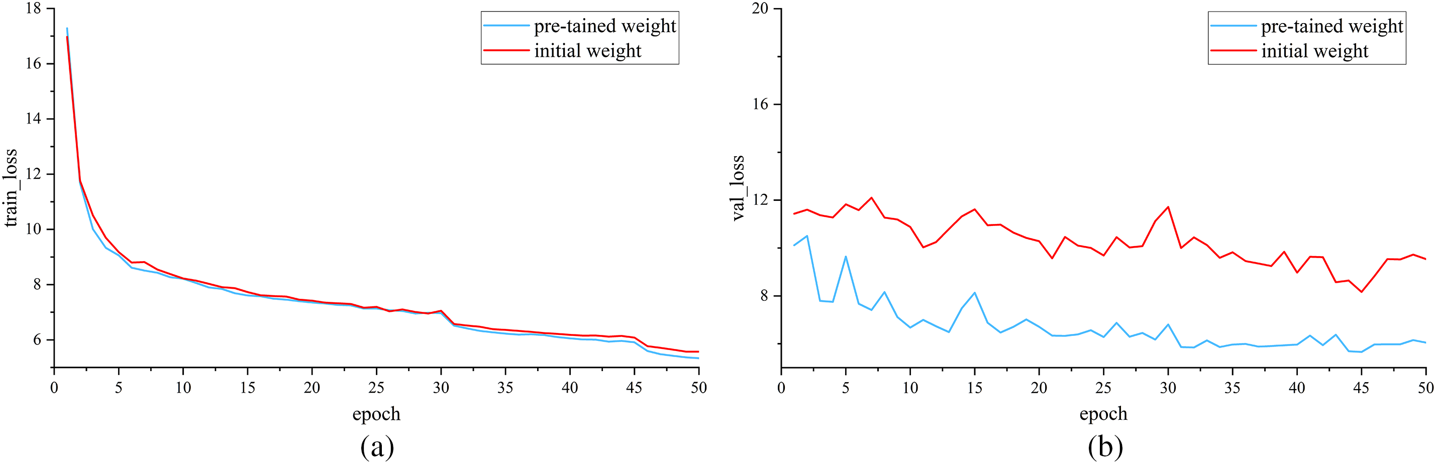
Figure 9: Loss comparison of initial and pre-trained weights: (a) Train loss; (b) Valid loss

To understand more intuitively the key regions that MSADCN focuses on during the feature extraction phase, we visualize the heat map. In Fig. 10, attention maps are from four skeletal development stages: prepubertal, early-mid, late, and post-pubertal [39]. The carpals and the mid-distal phalanges are the main targets of the prepubertal attentional map (a). Attention maps for early-mid and late adolescence (b and c) concentrate less on the carpal bones and more on the phalanges, suggesting that in patients during that time, their carpal bones are more significant predictors of BAA. Since the radius and ulna close last in the post-pubertal attention plot (d), focus more on the wrist bone [39]. As shown in Fig. 10, our proposed method validates this well. Therefore, relying on additional labels or manual extraction of ROI regions is not precise and challenging enough for BAA because the critical regions of hand bone used to characterize bone age differ for different ages. By visualizing the heat map, we can better understand which areas of the hand bone image are significant for BAA.

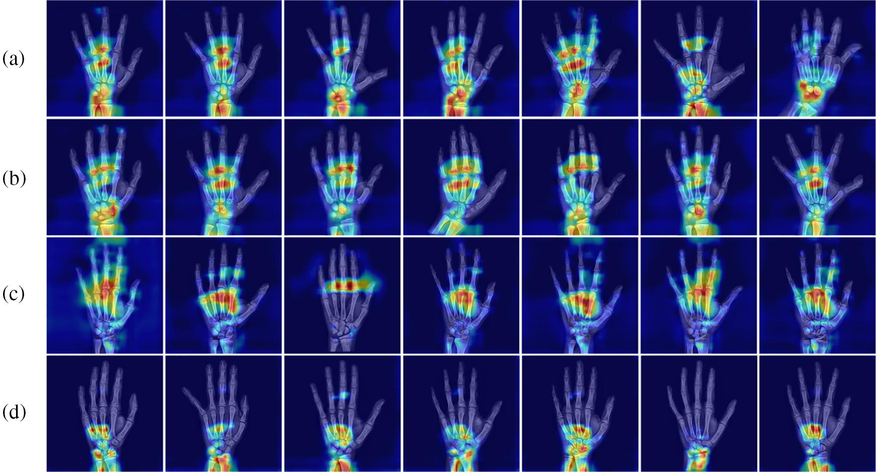
Figure 10: Heat map of the four stages of skeletal development: (a) Prepubertal, (b) Early-mid pubertal, (c) Late pubertal, (d) Post-pubertal

5  Discussion

5.1 Comparison with Advanced Methods

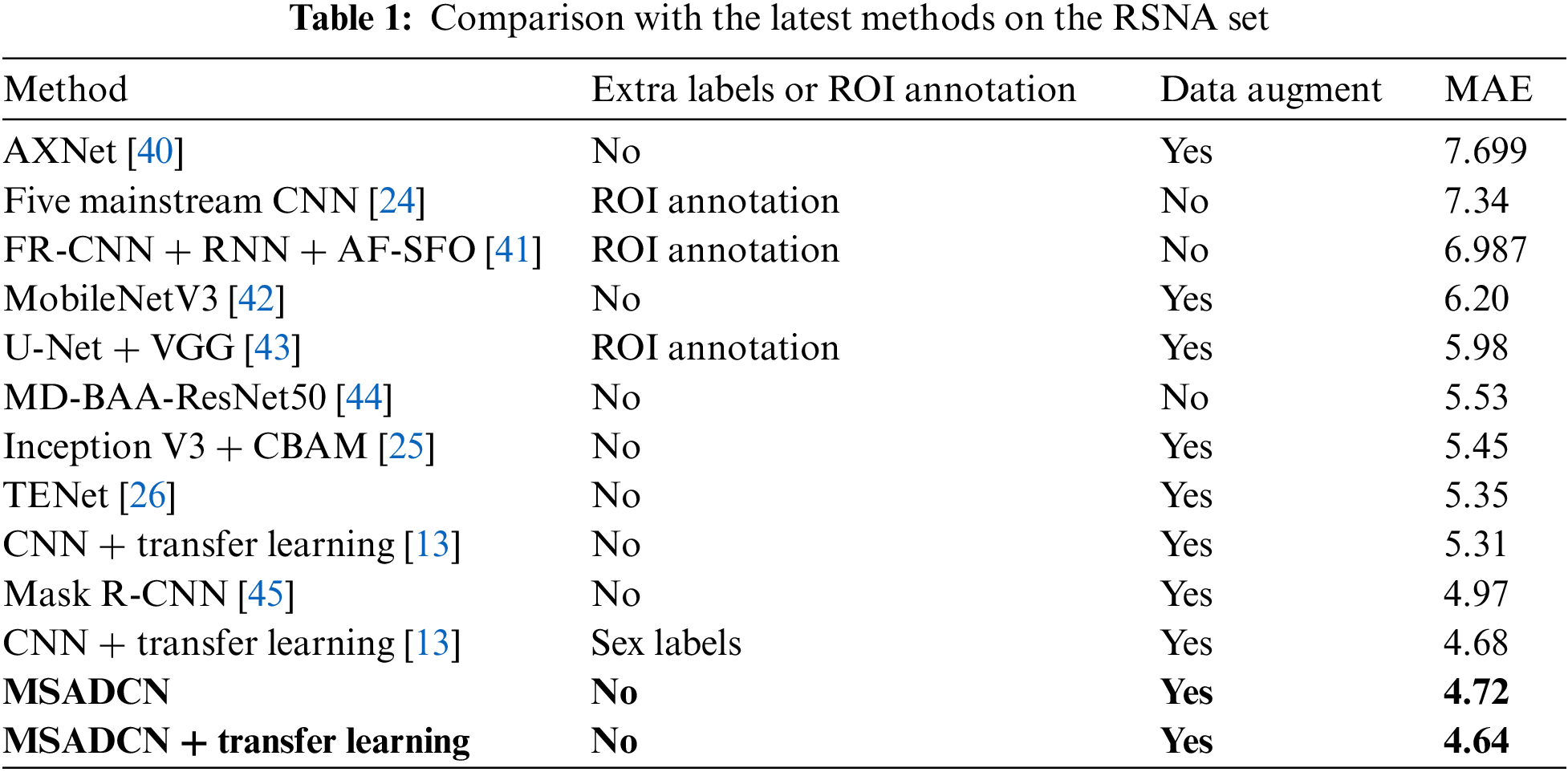
In this section, the performance of the proposed method will be compared to the state-of-the-art BAA methods [13,24–26,40–45]. From Table 1, we can observe that: (1) Current advanced BAA methods have promising results, but these methods depend on additional annotations such as sex labels or obtaining ROIs by segmentation [13,24,41,43]. (2) Our method without additional labels and transfer learning achieves superior results than [13] without providing additional annotations. In addition, the proposed method based on transfer learning also predicts better results than the [13] method that provides sex labels. (3) Compared to other neural networks, MSADCN can preserve the most information flow across layers, and each layer is subject to extra supervision, making the model converge more quickly. Besides, the multi-scale module within the dense layer can extract rich feature information while generating fewer parameters, and the attention mechanism between multi-scale dense blocks can significantly concentrate on the bone age features relevant to the model. Finally, the transfer learning-based MASDCN method can improve the model’s performance and obtain more robust prediction results. Overall, the proposed method is superior to some state-of-the-art methods.

5.2 Parameter Analysis

The network’s important parameters affect the model’s performance on the BAA task. To maximize the performance of the model, we analyze the impact of various hyperparameters, including scales, blocks, growth rate k, compression factor θ and loss coefficients λMAE and λKL.

Scales: In the feature extract stage of MSADCN, scales represent the multi-scale dimension of the 3 × 3 Conv in the multi-scale dense layer structure. The more multi-scale branches there are, the better the model can capture various image details and characteristics. However, too many branches will cause information loss and increase the model’s complexity. Fig. 11a depicts the influence of scales on the model. Under the same conditions (growth rate is 12, number of blocks is 3), the prediction result tends to be a concave function. When the number of scales is 8, the prediction is optimal, and the model’s performance reaches its peak.

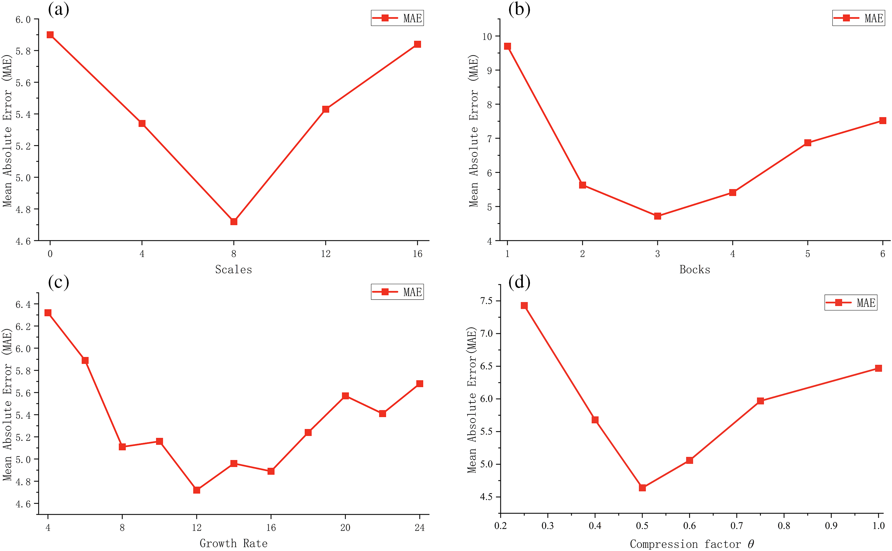
Figure 11: The effect of different hyperparameters on model performance: (a) Scales; (b) Blocks; (c) Growth rate k; (d) Compression factor θ

Number of blocks: Every two multi-scale dense blocks are connected by a transition layer, which has the effect of down-sampling and compressing the model. A proper sampling degree can make the model perform better, which depends on the number of multi-scale dense blocks. The experiments test the impact of the multi-scale dense blocks while keeping other parameters constant. As shown in Fig. 11b, when the dense blocks is 3, the model achieves the best prediction result for BAA.

Growth rate k: During the feature transfer process, each dense layer adds k feature maps to the next layer. As stated in Eq. (2), k determines how many feature maps each multi-scale dense layer produces. By fine-tuning the value of k while fixing other parameters, the experiment tests the effect of the growth rate on the model performance. Fig. 11c shows that a slight change in the growth rate significantly affects the BAA results. The reason is that k determines how many new features each dense layer contributes to the global state. Too large or too small will reduce the accuracy of the model prediction, i.e., the MAE value will be too large. As shown in Fig. 11c, the model performs best when k is about 32.

Compression factor θ: θ is a compression of the feature map size output from the previous multi-scale dense block by the transition layer, which serves to downsample and compress the model. The appropriate compression factor affects the model’s performance to some extent. Fig. 11d depicts the effect of different compression factors size of the prediction results. When the compression coefficient is 0.5, the prediction result is the best.

λMAE and λKL: The hyperparameters λMAE and λKL, which are used to balance the joint loss function in Eq. (18), impact the estimation of age by the model. Fig. 12 depicts the effect of λMAE and λKL of the bone age prediction results. The model tends to converge after 35 iterations when λKL is 1, and λMAE is 0.5. At this point, the prediction results obtained in the validation set are more accurate, which suggests that a proper trade-off between age distribution and expected regression can improve model performance and obtain more robust age predictions.

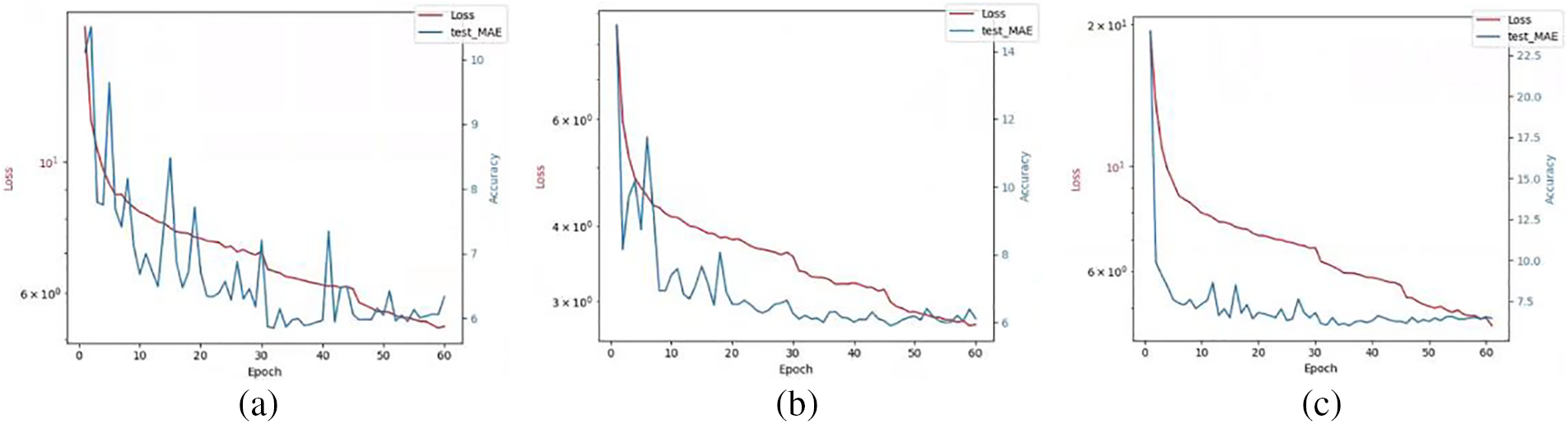
Figure 12: The effect of different loss coefficient values on model training: (a) λMAE=1, λKL=1; (b) λMAE=1, λKL=0.5; (c) λMAE=0.5, λKL=1

5.3 Ablation Experiments

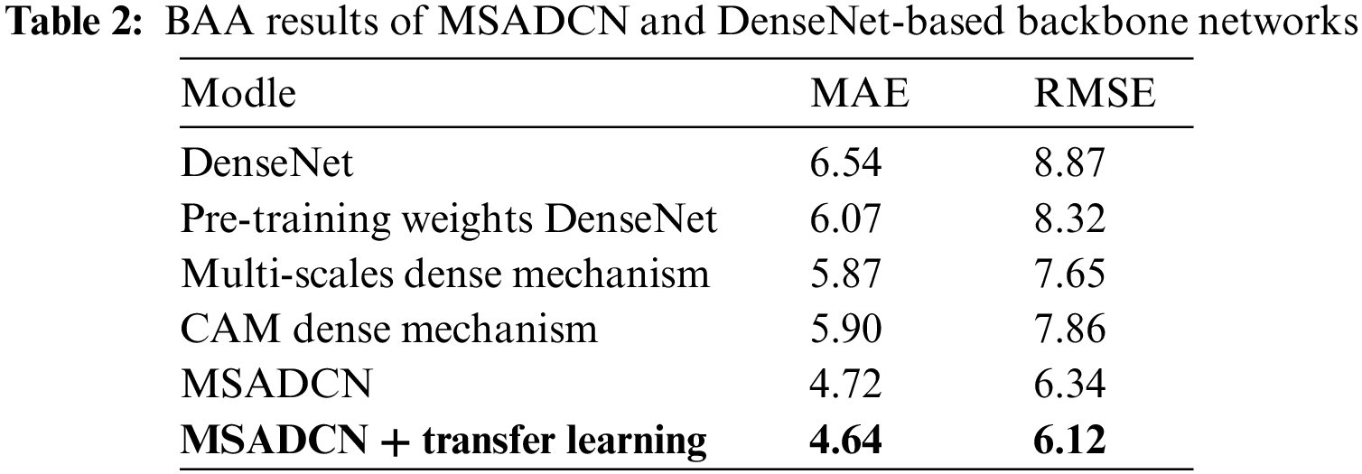
To validate the effectiveness of the proposed method for the BAA task, we evaluate the performance of each module of MSADCN on the RSNA dataset. Six different variants are constructed: (1) unmodified baseline DenseNet, (2) DenseNet load pre-trained weights, (3) multi-scale dense connectivity mechanism, (4) coordinate attention dense connectivity mechanism (CAM dense mechanism), (5) MSADCN, (6) MSADCN based on transfer learning.

Table 2 compares the MAE results with the above six variants respectively. We can see that: (1) DenseNet with pre-trained weights yields superior prediction results compared to DenseNet alone, which also has been confirmed by numerous. (2) Compared to DenseNet loaded with pre-trained weights, the densely connected mechanism combined with either the multi-scale module or CAM can obtain superior outcomes. It indicates that both can enhance the network’s ability to perceive features to a certain degree, thus further improving the model’s performance. (3) Compared to other methods, the proposed method performs best because it considers the fine-grained multi-scale level, and CAM can focus on the weight distribution during training. Besides, MSADCN based on transfer learning can further improve the model’s performance and generalization ability to a certain extent by loading the pre-trained weights on a large dataset.

6  Conclusions

A multi-scale attentional densely connected network based on transfer learning is proposed in this paper for the BAA task. Firstly, the model constructs a multi-scale dense connection mechanism that allows more efficient feature transfer with fewer parameters, which is less likely to suffer from overfitting and converges more quickly, even when the training dataset is limited. In addition, MSADCN extracts the features from the multi-scale level and employs coordinate attention to identify the discriminative regions of bone age features, making the extracted ROI more accurate and effective for model training. Finally, MSADCN based on transfer learning can significantly improve the model’s generalization ability by loading the pre-trained model, which provides a good research idea for medical image processing with limited data volume. Experiment results on the RSNA dataset confirm that our model can achieve comparable results.

Although current study has demonstrated the contribution of the proposed approach in BAA tasks, there are some limitations and uncertainties in this study. The model is more friendly to pre-processed hand bone images during training and predicts more accurate results. Therefore, there is a slight error in the predicted bone age for raw images with low resolution or high noise. In addition, the subject population of this study was the patients’ X-rays published by RSNA, and other populations are not currently available to be validated in the studied method. In future work, we will endeavor to collect additional data, and further investigate the effectiveness of BAA methods based on deep learning to assist orthopedic surgeons automatically and predict bone age objectively.

Acknowledgement: The authors would like to thank the anonymous editors and reviewers for their critical and constructive comments and suggestions.

Funding Statement: This research is partially supported by grant from the National Natural Science Foundation of China (No. 72071019), grant from the Natural Science Foundation of Chongqing (No. cstc2021jcyj-msxmX0185), and grant from the Chongqing Graduate Education and Teaching Reform Research Project (No. yjg193096).

Author Contributions: Study conception and design: Y. Yu, L. Yu, H. Zheng; Data collection: Y. Yu, H. Zheng; Analysis and interpretation of results: Y. Yu, H. Qi, Y. Deng; Draft manuscript preparation: Y. Yu, L. Yu. All authors have reviewed the results and approved the final version of the manuscript.

Availability of Data and Materials: The dataset used in this study is the public dataset RSNA which can be download from the link: https://www.kaggle.com/datasets/kmader/rsna-bone-age.

Conflicts of Interest: The authors declare that they have no conflicts of interest to report regarding the present study.

References

1. A. K. Poznanski, R. J. Hernandez, K. E. Guire, U. L. Bereza, and S. M. Garn, “Carpal length in childrena useful measurement in the diagnosis of rheumatoid arthritis and some congenital malformation syndromes,” Radiol., vol. 129, no. 3, pp. 661–668, 1978. doi: 10.1148/129.3.661. [Google Scholar] [PubMed] [CrossRef]

2. B. Büken, A. A. Şafak, B. Yazıcı, E. Büken, and A. S. Mayda, “Is the assessment of bone age by the Greulich-Pyle method reliable at forensic age estimation for Turkish children?,” Forensic. Sci. Int., vol. 173, no. 2–3, pp. 146–153, 2007. doi: 1010.1016/j.forsciint.2007.02.023. [Google Scholar] [PubMed] [CrossRef]

3. B. Büken, Ö. U. Erzengin, E. Büken, A. A. Şafak, B. Yazıcı, and Z. Erkol, “Comparison of the three age estimation methods: Which is more reliable for Turkish children?,” Forensic. Sci. Int., vol. 183, no. 1–3, pp. 103.e–103.e7, 2009. doi: 1010.1016/j.forsciint.2008.10.012. [Google Scholar] [PubMed] [CrossRef]

4. W. W. Greulich, and S. I. Pyle, “Radiographic atlas of skeletal development of the hand and wrist,” Am. J. Med. Sci., vol. 11, no. 3, pp. 282–283, 1959. [Google Scholar]

5. H. Carty, “Assessment of skeletal maturity and prediction of adult height (TW3 method),” Bone and Joint Journal, vol. 84, no. 2, pp. 310–311, 2002. doi: 1010.1302/0301-620X.84B2.0840310C. [Google Scholar] [CrossRef]

6. M. Niemeijer, B. van Ginneken, C. Maas, F. Beek, and M. Viergever, “Assessing the skeletal age from a hand radiograph automating the Tanner-Whitehouse method,” Med. Imaging2003: Image Process., vol. 5032, pp. 1197–1205, 2003. doi: 1010.1117/12.480163. [Google Scholar] [CrossRef]

7. R. de Luis-Garcia, M. Martín-Fernández, J. Arribas, and C. Alberola-López, “A fully automatic algorithm for contour detection of bones in hand radiographies using active contours,” in Proc. 2003 Int. Conf. Image Process., vol. 3, 2003. doi: 1010.1109/ICIP.2003.1247271. [Google Scholar] [CrossRef]

8. L. Pan, F. Zhang, Y. Yang, and C. Zheng, “Carpal bone feature extraction analysis in skeletal age assessment based on deformable model,” J. Comput. Sci. Technol, vol. 4, no. 3, pp. 152–156, 2004. doi: 1010.1007/BF01357541. [Google Scholar] [CrossRef]

9. D. Giordano, R. Leonardi, F. Maiorana, G. Scarciofalo, and C. Spampinato, “Epiphysis and metaphysis extraction and classification by adaptive thresholding and DoG filtering for automated skeletal bone age analysis,” in 29th Annu. Int. Conf. IEEE Eng. Med. Biol. Soc., 2007, pp. 6551–6556. [Google Scholar]

10. C. Spampinato, S. Palazzo, D. Giordano, M. Aldinucci, and R. Leonardi, “Deep learning for automated skeletal bone age assessment in x-ray images,” Med. Image. Anal., vol. 36, pp. 41–51, 2017. doi: 1010.1016/j.media.2016.10.010. [Google Scholar] [PubMed] [CrossRef]

11. Y. Liu, C. Zhang, J. Cheng, X. Chen, and Z. Wang, “A multi-scale data fusion framework for bone age assessment with convolutional neural networks,” Comput. Biol. Med., vol. 108, pp. 161–173, 2019. doi: 1010.1016/j.compbiomed.2019.03.015. [Google Scholar] [PubMed] [CrossRef]

12. K. Li et al., “Automatic bone age assessment of adolescents based on weakly-supervised deep convolutional neural networks,” IEEE Access, vol. 9, pp. 120078–120087, 2021. doi: 1010.1109/ACCESS.2021.3108219. [Google Scholar] [CrossRef]

13. Q. H. Nguyen, B. P. Nguyen, M. T. Nguyen, M. C. H. Chua, T. T. T. Do, and N. Nghiem, “Bone age assessment and sex determination using transfer learning,” Expert. Syst. Appl., vol. 200, pp. 116926, 2022. doi: 1010.1016/j.eswa.2022.116926. [Google Scholar] [CrossRef]

14. J. Seok, J. Kasa-Vubu, M. DiPietro, and A. Girard, “Expert system for automated bone age determination,” Expert Syst. Appl., vol. 50, pp. 75–88, 2016. doi: 1010.1016/j.eswa.2015.12.011. [Google Scholar] [CrossRef]

15. K. He, X. Zhang, S. Ren, and J. Sun, “Deep residual learning for image recognition,” in Proc. IEEE Conf. Comput. Vis. Pattern Recognit., 2016, pp. 770–778. [Google Scholar]

16. G. Larsson, M. Maire, and G. Shakhnarovich, “FractalNet: Ultra-deep neural networks without residuals,” arXiv preprint arXiv:1605.07648, 2016. [Google Scholar]

17. R. K. Srivastava, K. Greff, and J. Schmidhuber, “Training very deep networks,” Adv. Neural Inf. Process. Syst., vol. 28, pp. 2377–2385, 2015. [Google Scholar]

18. H. H. Thodberg, S. N. Kreiborg, A. Juul, and K. D. Pedersen, “The bonexpert method for automated determination of skeletal maturity,” IEEE Trans. Med. Imaging., vol. 28, no. 1, pp. 52–66, 2008. doi: 1010.1109/TMI.2008.926067. [Google Scholar] [PubMed] [CrossRef]

19. M. Kashif, S. Jonas, D. Haak, and T. M. Deserno, “Bone age assessment meets SIFT,” in Medical Imaging 2015: Computer-Aided Diagnosis, Orlando, Florida, USA, SPIE, 2015, vol. 9414, pp. 792–798. [Google Scholar]

20. A. Kumar, “Study and analysis of different segmentation methods for brain tumor MRI application,” Multimed. Tools. Appl., vol. 82, no. 5, pp. 7117–7139, 2023. doi: 1010.1007/s11042-022-13636-y. [Google Scholar] [PubMed] [CrossRef]

21. S. Dhyani, A. Kumar, and S. Choudhury, “Arrhythmia disease classification utilizing ResRNN,” Biomed. Signal. Process. Control, vol. 79, pp. 104160, 2023. doi: 1010.1016/j.bspc.2022.104160. [Google Scholar] [CrossRef]

22. A. S. Rawat, A. Ran, A. Kumar, and A. Bagwari, “Application of multi layer artificial neural network in the diagnosis system: A systematic review,” IAES Int. J. Artif Intell., vol. 7, no. 3, pp. 138–142, 2018. doi: 1010.1109/RICE.2018.8509069. [Google Scholar] [CrossRef]

23. H. Lee et al., “Fully automated deep learning system for bone age assessment,” J. Digit. Imaging, vol. 30, pp. 427–441, 2017. doi: 1010.1007/s10278-017-9955-8. [Google Scholar] [PubMed] [CrossRef]

24. Y. Deng et al., “Bone age assessment from articular surface and epiphysis using deep neural networks,” Math. Biosci. Eng., vol. 20, no. 7, pp. 13111–13148, 2023. doi: 1010.3934/mbe.2023585. [Google Scholar] [PubMed] [CrossRef]

25. Z. Li et al., “Bone age assessment based on deep neural networks with annotation-free cascaded critical bone region extraction,” Front. Artif. Intell., vol. 6, pp. 1142895, 2023. doi: 1010.3389/frai.2023.1142895. [Google Scholar] [PubMed] [CrossRef]

26. K. Jian, S. Li, M. Yang, S. Wang, and C. Song, “Multi-characteristic reinforcement of horizontally integrated TENet based on wrist bone development criteria for pediatric bone age assessment,” Appl. Intell., vol. 53, pp. 22743–22752, 2023. doi: 1010.1007/s10489-023-04633-1. [Google Scholar] [CrossRef]

27. J. Fu, H. Zheng, and T. Mei, “Look closer to see better: Recurrent attention convolutional neural network for fine-grained image recognition,” in Proc. IEEE Conf. Comput. Vis. Pattern Recognit., 2017, pp. 4438–4446. [Google Scholar]

28. C. Chen, Z. Chen, X. Jin, L. Li, W. Speier, and C. W. Arnold, “Attention-guided discriminative region localization and label distribution learning for bone age assessment,” IEEE J. Biomed. Health Inform., vol. 26, no. 3, pp. 1208–1218, 2021. doi: 1010.1109/JBHI.2021.3095128. [Google Scholar] [PubMed] [CrossRef]

29. M. A. Zulkifley, N. A. Mohamed, S. R. Abdani, N. A. M. Kamari, A. M. Moubark, and A. A. Ibrahim, “Intelligent bone age assessment: An automated system to detect a bone growth problem using convolutional neural networks with attention mechanism,” Diagnostics, vol. 11, no. 5, pp. 765, 2021. doi: 1010.3390/diagnostics11050765. [Google Scholar] [PubMed] [CrossRef]

30. X. Ren et al., “Regression convolutional neural network for automated pediatric bone age assessment from hand radiograph,” IEEE J. Biomed. Health Inform., vol. 23, no. 5, pp. 2030–2038, 2018. doi: 1010.1109/JBHI.2018.2876916. [Google Scholar] [PubMed] [CrossRef]

31. V. Iglovikov, A. Rakhlin, A. Kalinin, and A. Shvets, “Paediatric bone age assessment using deep convolutional neural networks,” Deep Learn. Med. Image Anal. Multimodal Learn. Clin. Decis. Support, vol. 11045, pp. 300–308, 2018. doi: 1010.1007/978-3-030-00889-5_34. [Google Scholar] [CrossRef]

32. S. Gao, M. Cheng, K. Zhao, X. Zhang, M. Yang, and P. Torr, “Res2Net: A new multi-scale backbone architecture,” IEEE Trans. Pattern Anal. Mach. Intell., vol. 43, no. 2, pp. 652–662, 2019. doi: 1010.1109/TPAMI.2019.2938758. [Google Scholar] [PubMed] [CrossRef]

33. G. Huang, Z. Liu, L. V. der Maaten, and K. Q. Weinberger, “Densely connected convolutional networks,” in Proc. IEEE Conf. Comput. Vis. Pattern Recognit., 2017, pp. 4700–4708. [Google Scholar]

34. Q. Hou, D. Zhou, and J. Feng, “Coordinate attention for efficient mobile network design,” in Proc. IEEE/CVF Conf. Comput. Vis. Pattern Recognit., 2021, pp. 13713–13722. [Google Scholar]

35. R. Müller, S. Kornblith, and G. E. Hinton, “When does label smoothing help?,” in Advances in Neural Information Processing Systems, Vancouver Convention Center, Vancouver, Canada, NeurIPS, 2019, pp. 4694–4703. [Google Scholar]

36. Z. Huo et al., “Deep age distribution learning for apparent age estimation,” in Proc. IEEE Conf. Comput. Vis. Pattern Recognit. Workshops, 2016, pp. 17–24. [Google Scholar]

37. X. Geng, “Label distribution learning,” IEEE Trans. Knowl. Data Eng., vol. 28, no. 7, pp. 1734–1748, 2016. doi: 1010.1109/TKDE.2016.2545658. [Google Scholar] [CrossRef]

38. B. Gao, C. Xing, C. Xie, J. Wu, and X. Geng, “Deep label distribution learning with label ambiguity,” IEEE Trans. Image Process., vol. 26, no. 6, pp. 2825–2838, 2017. doi: 1010.1109/TIP.2017.2689998. [Google Scholar] [PubMed] [CrossRef]

39. V. Gilsanz, and O. Ratib, Hand Bone Age: A Digital Atlas of Skeletal Maturity. Springer Berlin, Heidelberg, Springer Science & Business Media, 2005. [Google Scholar]

40. M. Zulkifley, N. Mohamed, S. Abdani, and N. A. M. Kamari, “Intelligent bone age assessment: An automated system to detect a bone growth problem using convolutional neural networks with attention mechanism,” Diagnostics, vol. 11, no. 5, pp. 765, 2022. doi: 1010.3390/diagnostics11050765. [Google Scholar] [PubMed] [CrossRef]

41. D. Sonal, and K. Arti, “Faster region-convolutional neural network oriented feature learning with optimal trained Recurrent Neural Network for bone age assessment for pediatrics,” Biomed. Signal Proces. Control, vol. 71, pp. 103016, 2022. doi: 1010.1016/j.bspc.2021.103016. [Google Scholar] [CrossRef]

42. S. Li, B. Liu, S. Li, X. Zhu, Y. Yan, and D. Zhang, “A deep learning-based computer-aided diagnosis method of x-ray images for bone age assessment,” Complex Intell. Syst., vol. 8, pp. 1929–1939, 2022. doi: 1010.1007/s40747-021-00376-z. [Google Scholar] [PubMed] [CrossRef]

43. B. Liu, Y. Zhang, M. Chu, X. Bai, and F. Zhou, “Bone age assessment based on rank-monotonicity enhanced ranking CNN,” IEEE Access, vol. 7, pp. 120976–120983, 2019. doi: 1010.1109/ACCESS.2019.2937341. [Google Scholar] [CrossRef]

44. H. Tang, X. Pei, X. Li, H. Tong, X. Li, and S. Huang, “End-to-end multi-domain neural networks with explicit dropout for automated bone age assessment,” Appl. Intell., vol. 53, pp. 3736–3749, 2022. doi: 1010.1007/s10489-022-03725-8. [Google Scholar] [CrossRef]

45. Z. Q. Liu et al., “Bone age recognition based on mask R-CNN using xception regression model,” Front. Physiol., vol. 14, pp. 1062034, 2023. doi: 1010.3389/fphys.2023.1062034. [Google Scholar] [PubMed] [CrossRef]