Predicting Traffic Flow Using Dynamic Spatial-Temporal Graph Convolution Networks

1  Introduction

With the improvement of the modernization level and the continuous advancement of urbanization, lots of new vehicles are projected onto the road, these cause serious traffic security, result in critical traffic jams, and prolong the traffic time of people. To deal with complex traffic problems, Intelligent Transportation systems (ITS) have emerged. Traffic flow prediction is the key task of ITS. Timely and accurate traffic prediction results can not only relieve traffic congestion, increase traffic efficiency, and decrease energy consumption and pollution but also be the basis and premise of new applications across the traffic field.

Traffic forecasting research has been going on for decades. Early works focus on statistical methods, such as historical average (HA) [1], autoregressive integrated moving average (ARIMA) [2], vector autoregressive (VAR) [3], and Kalman filter [4], etc. Although these methods can capture the temporal dependency of traffic data, they neglect the spatial relation and limit their applications. Later, deep learning models, such as stacked self-coding machines, deep belief network (DBN) [5], long short-term memory network (LSTM) [6] and gated recurrent unit (GRU) [7] have achieved improvement in prediction accuracy because they can learn the non-linearity and complex spatial-temporal dependencies of traffic models. Besides the recurrent neural network (RNN), convolutional neural network (CNN) is widely employed to recognize the spatial and temporal relationships of traffic flow. Afterward, the attention mechanism is widely used for traffic prediction. Though these models can obtain satisfactory results when processing Euclidean data, these models are highly constrained in traffic flow prediction because the traffic data usually follow a non-Euclidean structure. Afterward, the graph convolutional network (GCN) stands out among various traffic prediction models and has achieved considerable accuracy. The latest research works have applied GCN [8], GAT [9], and GNN [10] to cope with the traffic forecasting problem.

Most of the existing studies are based on graph neural networks to model traffic flow graphs, and the fixed graph structure is usually applied to deal with the relationship between nodes. However, due to the time-varying spatial correlation of the traffic network, there is no fixed relationship between the traffic nodes, and these methods cannot effectively integrate the spatio-temporal characteristics.

To address these issues, the paper proposed TSADGCN, a novel traffic flow prediction model based on a temporal-spatial relationship graph and attention mechanism network. TSADGCN deeply explores the complex temporal and spatial characteristics of traffic flow data and establishes their dependence relationship, combining with attention mechanism and dilated gated convolution network (DGCN) [11], and improves the prediction accuracy of traffic flow. According to the similarity of traffic flow sequences between road nodes in the temporal dimension, the concept of a time graph is proposed. The similarity is calculated by the DTW algorithm [12]. Based on the spatial-temporal relationship graph, graph convolution and time dimension convolution are performed separately on each branch with attention mechanism, respectively, to capture the spatial-temporal characteristics of the traffic flow and its dependence relationship, and then the spatial-temporal relationship of the traffic flow data is modeled.

The main contributions of this work are described as follows:

•   A dilated and gating convolution is proposed to achieve deep temporal features with long receptive fields, based on a spatial self-attention mechanism, and the node correlation of the real spatial relationship is calculated.

•   The design is a set of adaptive graphs: A time graph with an adjacency matrix as prior information and a spatial graph with a sequential association matrix to capture dynamic real node dependencies. The DTW algorithm is used to calculate the similarity degree of traffic flow sequence between nodes in the road network in time dimension, and the concept of time graph is proposed. Based on the spatio-temporal relationship diagram, the graph convolution and temporal dimension convolution are respectively carried out in each branch combined with the attention mechanism to capture the spatio-temporal characteristics of traffic flow and their dependencies, and realize the modeling of the spatio-temporal relationship of road network traffic flow data.

•   On the public data set PeMSD4 and PeMSD8 the model proposed in this paper is experimentally verified and the performance is compared with common predictive models. Experiments show that the MAE and RMSE of the TSADGCN are respectively better than those of ARIMA, STGCN, and ASTGCN.

The remainder of this article is organized as follows. Section 2 describes the theoretical background. Section 3 formulates the problem definitions and defines the notations. Section 4 discusses the proposed model in detail. Section 5 details the experimental design. Section 6 illustrates experimental results. Finally, Section 7 concludes this paper, and the potential future work is suggested.

2  Related Works

2.1 Traditional Prediction Methods of Traffic Flow

Traditional prediction methods aim to mine the rule of temporal dimension from the traffic flow sequence. These methods include parameter models and non-parameter models. Parameter models consist of ARIMA, Kalan filter, etc. Non-parameter models include k-nearest neighbor (KNN), support vector machine (SVM), and Bayes networks [13]. Traditional forecasting methods usually require the temporal sequence to satisfy certain periodicity and regularity. However, owing to its non-linearity and randomness, the efficiency of traditional methods is not ideal.

2.2 Traffic Flow Prediction Methods Based on Euclidean Convolutional Networks

Many researchers have employed Euclidean convolutional networks to forecast traffic flow. Combining the Residual network with CNN, Zhang et al. [14] proposed a novel temporal-spatial data prediction model for forecasting the city population flow. DBN [5] can effectively capture the high-dimension features of traffic data and decrease the forecasting error. WaveNet [15] was applied to build a spatial-temporal graph. By constructing a new self-adaptive dependency matrix and learning it by node embedding, the model can automatically and accurately capture unseen graph structure from traffic data. However, Euclidean convolutional models are difficult to directly apply to graph-structure data, so unable to deal with the graph-structure information of the traffic data.

2.3 Traffic Flow Methods Based on Graph Convolutional Network

Recently, GCN has obtained wide attention in traffic flow prediction and graphs have been used to construct models of non-Euclidean traffic flow data.

Guo et al. [16] proposed a novel model combining attention mechanism and temporal-spatial convolutional network to deal with traffic flow forecasting problem, using temporal-spatial attention mechanism to capture dynamic spatial-temporal correlation in traffic flow data. Yu et al. [17] developed the STGCN model and employed a graph to build the convolutional structure problem. GMAN [18] employed an encoder-decoder framework to simulate the effect of spatial-temporal factors on traffic conditions. T-GCN [19] used the hop links scheme to capture the periodic time correlation and add the residual to the recurrent graph network, to improve the problem of gradient explosion and disappearance in long-term backpropagation in deep networks. AST-GCN [20] combines spatial-temporal graph convolutional models to capture external information while integrating dynamic and static external information related to roads, such as weather and surrounding landmarks.

There are many transport management solutions to resolve the challenges resulting in traffic congestion. Jain et al. [21] proposed Real-Time Vehicle Data Integration (RTVDI), which utilized real-time vehicle data to reduce congestion. RTVDI uses SVM to collect real-time data from vehicles and use other machine learning algorithms and statistical approaches to acquire insights into traffic patterns and circumstances and pinpoint locations. Compared with RTVDI, the paper proposed TSADGCN uses both graph attention networks and temporal attention networks to predict the traffic flow, the prediction model is more complex and the prediction accuracy is higher than that of RTVDI. In addition, TSADGCN uses the DTW algorithm to calculate the similarity of traffic flow sequences between road nodes in the time dimension. ATM [22] can constantly update traffic signal schedules depending on traffic volume and estimated movements from nearby crossings. ATM utilizes the machine-learning-based DBSCAN clustering method to detect any accidental anomaly. Compared with ATM, the TSADGCN Model uses static data, and input data flow is divided into three parts: Adjacent data fragment, recent data fragment, and historical data fragment to extract features.

In summary, existing graph convolutional models usually pay attention to the temporal dimension or spatial dimension relationships, fail to consider the dependency among traffic nodes at different timestamps, and the possible dependencies between different nodes at different time intervals are not fully considered. In addition, most algorithms are based on graph neural networks to model traffic graphs and attempt to use fixed graph structures to obtain relationships between nodes.

3  Problem Formalization

In this paper, the traffic prediction task is to learn a function that maps signals from T historical graphs to future T’ graphs, i.e., to predict the traffic state in a future time interval based on the traffic information in the past time interval.

To represent the forecasting process, give some definitions as follows:

Definition 1 (Road graph). A road graph G = (V,E) is used to denote the connection relationship between road nodes. Where V∈RN×M is a set of nodes, M denotes the number of the characteristic at each node, E is the edges set representing the connection between nodes.

Definition 2 (Adjacency Matrix). The adjacency matrix AM is defined as the collective characteristic of the road map, representing the connectivity of the road network, which can be formalized as

AM(i,j)={1, AM(i,j)=10, otherwise(1)

Let Xt∈RN×M denote the observation of N nodes at time point t, and let Xti∈R denote the observation of the ith node at time point t. Given a series of node historical observations at S time points X = {Xt−S,Xt−S+1,L,Xt}, the target of traffic prediction is to predict a series of observations Y = (Xt+1,Xt+2,⋯,Xt+Tp), where Tp is a special time point after the current time. We strive to build a mapping function f(⋅) between 𝒳 and 𝒴 to minimize the loss, f:[X(t−T+1),…,Xt;G]→[X(t+1),…,X(t+Tp)].

4  TSADGCN Framework

The proposed TSADGCN framework in this paper is depicted in Fig. 1. The framework comprises a temporal sequence split module, temporal convolutional networks layer with attention mechanism, DGCN layer, spatial convolutional layer with attention mechanism (SGCN), and temporal-spatial graph and weighted fusion module.

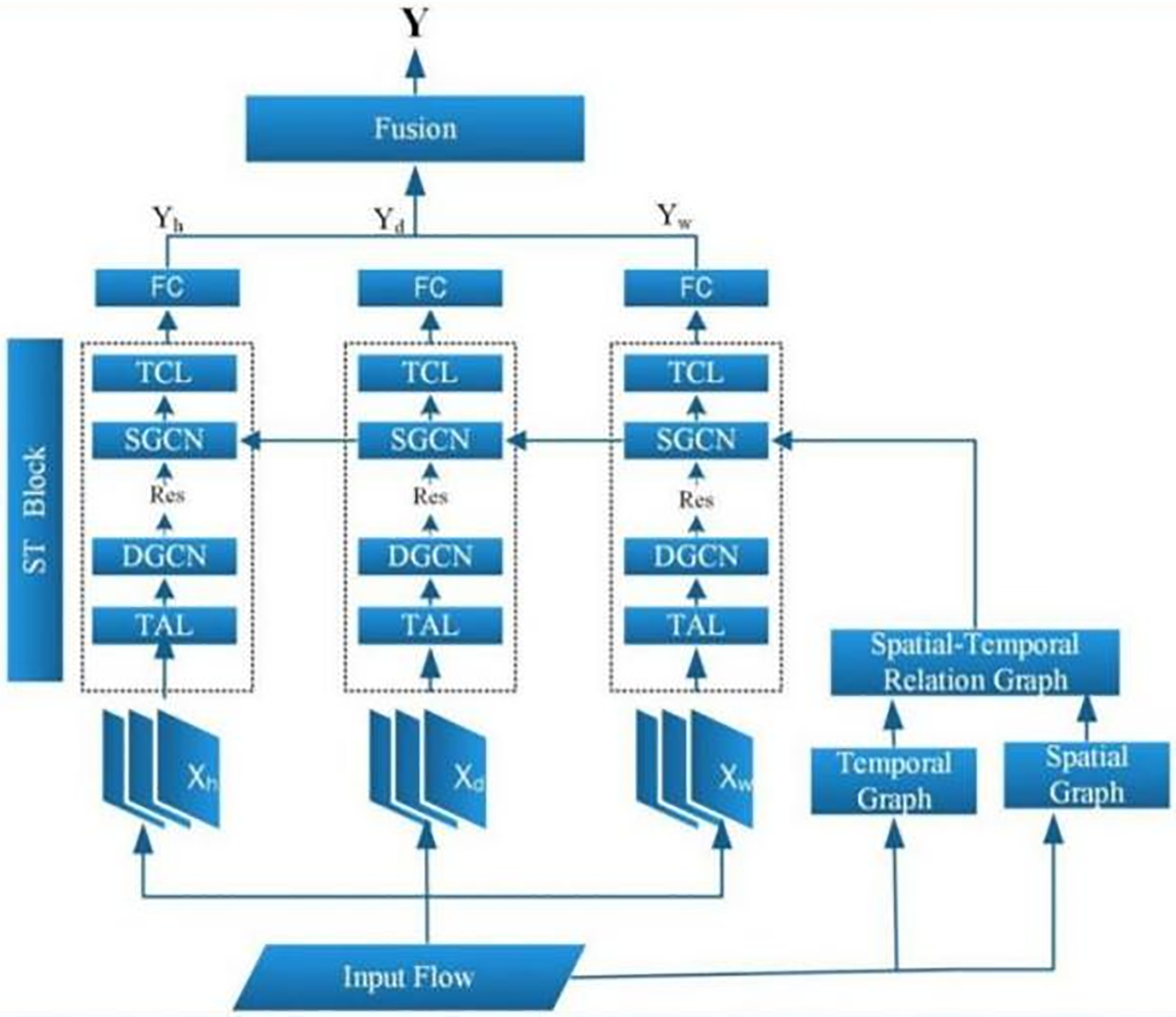
Figure 1: Framework of TSADGCN

Input flow is a traffic data set. Xh,Xd and Xw are respectively adjacent data fragments, recent data fragments, and historical data fragments. The spatial-temporal diagram is formed by fusing the time graph established by the DTW algorithm and the spatial graph established according to the neighborhood relationship between nodes. Based on the spatial-temporal relationship graph, graph convolution and time dimension convolution are performed separately on each branch with attention mechanism, respectively, to capture the spatial-temporal characteristics of the traffic flow and its dependence relationship, and then the spatial-temporal relationship of the traffic flow data was modeled. Fusion is weighted output. Ψs,h,Ψs,d,Ψs,w are spatial attention weight matrix of three modules, respectively. Yh,Yd and Yw are the traffic flow predictions of the three modules, respectively. FC is the full connection layer, and Y is eventually the traffic flow output.

4.1 Input Flow Split

Considering the periodicity, proximity, and other characteristics of traffic flow data in the temporal dimension, the input flow is divided into three parts: Adjacent data fragment, recent data fragment, and historical data fragment to extract features. As shown in Fig. 2, taking the traffic flow predicting X(T) after Tx time step as an example, the input sequence is split as follows.

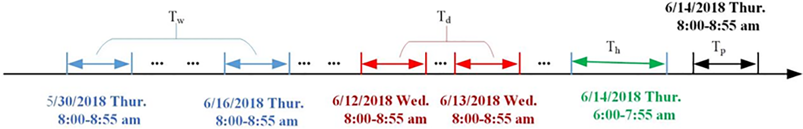
Figure 2: An example of constructing the input of time sequence fragments

Adjacent data fragment Xh = {XT−h,XT−h+1,...,XT−1}∈RN×M×Th is the historical data near the predicted value. The recent data fragment Xd={XT−p,XT−p+1,…,XT−p+Tx}∈RN×M×Td is historical data for the previous 1 day at the same time as the forecast fragment. A historical data fragment Xw={XT−w,XT−w+1,…,XT−w+Tx}∈RN×M×Tw is historical data from one week ago at the same time as the forecast period. Where Tx = 12, the traffic flow data is predicted for the next 1 h; h = 36, the traffic flow data for the first 3 h of the segment to be predicted is selected; p is the traffic flow data for that moment in the day before the segment to be predicted; w is the traffic flow data for that moment in the previous week.

4.2 Spatial-Temporal Block

To capture the structure features at the temporal dimension and spatial dimension, in this paper, three spatial-temporal components are used to explore and analyze the spatial-temporal relationships between historical data sequence, recent data sequence, and adjacent data sequence. The spatial-temporal component consists of the attention mechanism, DGCN, and graph attention network.

4.2.1 Temporal Attention Layer

The traffic flow has related change within a period. The attention model can allocate different weights and obtain dynamic temporal relationships according to traffic flow data. Meanwhile, the noise ratio is reduced accordingly. Different kinds of data are input into the attention layer for deep fusion to obtain a more credible attention weight. Attention weight can be calculated as follows:

E = Ve⋅σ(((Xhr)TU1)U2(U3Xhr)+be)(2)

Ep,q ′ = softmax(Ep,q)=exp⁡(Ep,q)∑q=1Trexp⁡(Ep,q)(3)

where Ve,be∈RTr×Tr, U1∈RN, and U3∈RCr are learnable parameters. Xhr={X1,X2,…,XTr−1}∈RN×Cr×Tr represents the output of the rth spatial-temporal block and the input of the rth+1 spatial-temporal block, respectively. E represents the number of attention scores at each time t and varies with the input data. Ep,q denotes the correlation between time P and time Q and normalized using the Softmax function.

4.2.2 DGCN

In this paper, DGCN is mainly applied to achieve deep temporal features and dependencies. DGCN is a temporal convolutional layers that have the advantages of dilated convolution and gating mechanisms. The gated mechanism is the key component of DGCN. The aim of using the residual structure is to prevent gradients from disappearing during the deepening of the network, while allowing more information to be transmitted across multiple features. Dilated convolution is another key component of DGCN, whose internal process is shown in Fig. 3. The receive field increases with the dilated ratio, and it is very useful for long-term prediction. A uniformly distributed random tensor is defined to perturb the gate of DGCN. The input of this layer is X^h∈RN×Cr×Tr, and X^hr is the output from the attention layer after the rth layer.

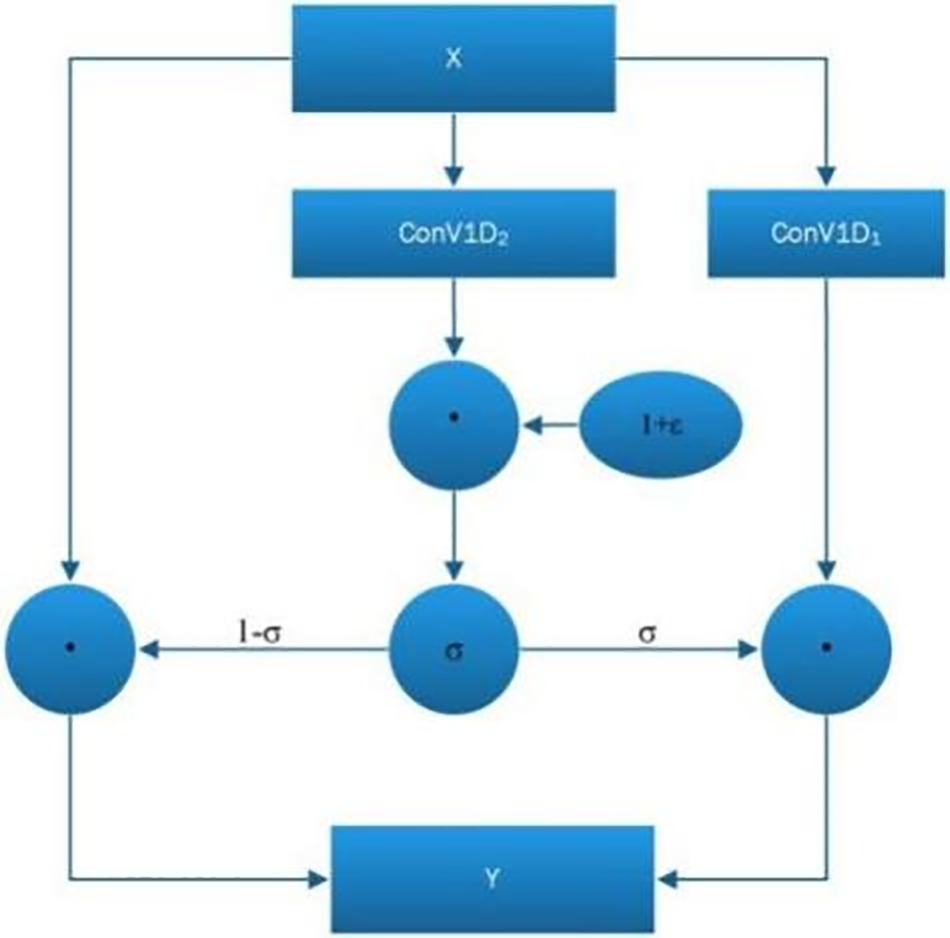
Figure 3: Structure of DGCN

4.2.3 Construct Spatial-Temporal Relationship Graph

The DTW is a typical algorithm for calculating the similarity of a two-time sequence, and this paper uses DTW ideas to construct a time association matrix of traffic flow data between different nodes. For any two nodes i and j, the traffic sequence is represented as

{Xi,f=(xi,1,f,xi,2,f,⋯,xi,l,f)Xj,f=(xj,1,f,xj,2,f,⋯,xj,l,f)(4)

where Xi,f,Xj,f denote respectively the traffic flow data of node i and node j, I and J is the length of two sequence.

Euclidean distance between middle points of two sequences is used to measure the similarity, let d(m,l) represents the Euclidean distance function.

d(m,l)=|xi,m,f−xj,l,f|,m∈[1,I];l∈[1,J](5)

where m, l are the mth, lth timestamps in the traffic flow sequence of node i and node j, respectively.

Let path P=(P1,P2,L,PE) as outline path diagram between the two sequences, is shown in Fig. 4.

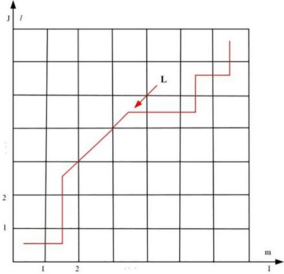
Figure 4: Outline path diagram

The whole path meets the constraint conditions:

{lk=(mk,lk)∈[1,I]×[1,J]l1=(1,1) and lE=[I,J]0≤mk+1−mk≤10≤lk+1−lk≤1(6)

where lk=(sk,tk) is the coordinates of the points passed in the path in Fig. 4.

The total matching cost between two sequences is defined as

C(Xi,f,Xj,f)=∑k=1Ed(sk,tk)=∑k=1E|xi,sk,xj,tk|(7)

In this paper, the minimum total matching cost is defined recursively as

C(sk,tk)=d(sk,tk)+min[C(sk,tk−1)+C(sk−1,tk)+C(sk−1,tk−1)](8)

Finally, the minimum matching cost C(I,J) is defined as

C(I,J)=DTW(Xi,f,Xj,f)=min[C(Xi,f,Xj,f)](9)

Definition 3 (Temporal graph) A temporal graph GT(V,D) comprises a set of road nodes V and a set of edges D representing the set of time sequence similarity degrees between each node, which is shown in Fig. 5.

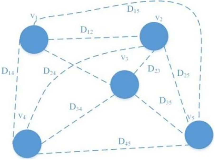
Figure 5: Time graph

Definition 4 (Time sequence association matrix). Given the timing sequence similarity threshold, the time sequence association matrix is a location characterization of nodes, which can be formalized as

AM0(i,j)={1,Di,j<TThreshold0,otherwise(10)

where TThreshold is used to distinguish whether the time series between two nodes is similar. The time sequence within the threshold is considered to be similar.

Definition 5 (Spatial-temporal relation graph) A spatial-temporal relation graph GT(V,AMs) consists of V and AMs represents the matrix merging adjacent matrix and temporal incidence matrix.

AMs(i,j)={1,AM(i,j)=1orAM0(i,j)=10,otherwise(11)

The spatial-temporal diagram is shown in Fig. 6.

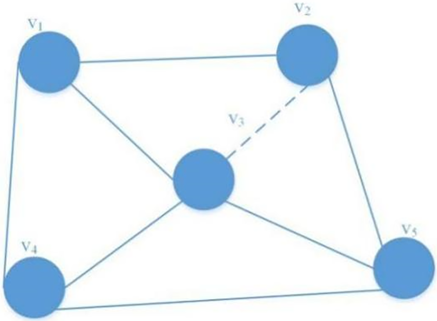
Figure 6: GT diagram

4.2.4 Spatial Attention Weight

Considering the influence of each node on the traffic flow and the interaction between different nodes, the attention mechanism is added to measure the importance of input features of different nodes and input features at different times.

Double-linear attention is applied to design the score function. Given as Xd spatial correlation Γv,d is defined as

Γv,d=Sv,d×σ[(XdW1,d)W2,d(W3,dXd)T+bv,d](12)

where Sv,d∈RN×N,bv,d∈RN×N,W1,d∈RH,W2,d∈RM×H,W3,d∈RM are the parameters to be learned, W1,d represents the weight of the H dimension, W3,d and denotes the weight of different data types. W2,d characterizes the interaction between the H dimension and the dimension weights of different data kinds. W3,c represents the weight of different data types, such as the weight of vehicle speed in flow prediction, etc. W2,c represents the interaction between dimension H and dimension weights of different data types, Xc∈RN×F×H is all data of all nodes, σ is the activation function, N is number of nodes, F is the number of data types, H is the length of time. For H selection of the three branches of adjacent information, recent information, and historical information, the first three time points, the same time point of the previous day and the same time point of the previous week, have the most obvious historical influence on the current traffic flow.

According to the spatial correlation matrix, then take the attention weight matrix of the adjacent information branch space as an example, the expression of the spatial attention weight between node i and node j is formulated as follows:

αV(i,j),d=exp⁡(ΓV(i,j),d)∑j=1Nexp⁡(ΓV(i,j),d)(13)

ΓV(i,j),d is the element in row i and column j of the spatial correlation matrix, which represents the spatial dimension correlation degree between node i and node j. αV(i,j),d is the spatial attention weight of node i and node j. By calculating the spatial attention weights of all nodes, the spatial attention weight matrix can be obtained.

Ψs,d=(αv(1,1),dαv(1,2),d…αv(1,N),dαv(2,1),dMαv(2,2),dOαv(2,N),dMαv(N,1),dLαv(N,N),d)(14)

The spatial attention weight matrices of the other two branches Ψs,hΨs,w can also be obtained.

4.2.5 SGCN

In this paper, SGCN is mainly applied to achieve not only the spatial relationship in the road network structure but also the time-dimensional relationship and space-time correlation feature of sequence similarity between nodes. Based on establishing the spatial-temporal diagram, the spatial dimension characteristics of the nodes in the space-time graph are extracted by graph convolution. This feature combines nThe entire graph is represented by its corresponding Laplacian matrix, and the Laplacian matrix L of the space-time graph is defined as follows:

L=IN−Ds−12AMsDs−12(15)

Ds=∑jAs(i,j)(16)

where AMs is the neighbor matrix for Section 4.2.3, In is the identity matrix.

Performing the eigenvalue decomposition on L, then L=βΔβT, where Δ is the diagonal matrix formed by the eigenvalues of L, and β is the decomposition basis. Using the above parameters, the formula for graph convolution on the input historical data is obtained as

Xg=βΘg(Δ)βTX(17)

where Θg is the convolution kernel parameter of the graph and Xg is the convolution result of the graph.

The first-order Chebyshev polynomial is used to approximately reduce the Eq. (18).

Xg≈θg[IN+D−12(IN+As)D−12]X(18)

where θg∈R is a trainable parameter.

Using the above graph convolution calculation method, combined with the spatial attention weight matrix in Section 4.2.3, the result of the spatial-temporal relationship graph convolution combined with the attention mechanism can be obtained as follows:

Xd,g≈θd,g[IN+D−12(IN+As)D−12]⊙ΨS,d(19)

where ⊙ is the Hadamard product. According to the above method, the outputs Xh,g, and Xw,g of the three branches after spatial-temporal graph convolution can be calculated in turn.

4.2.6 Temporal Convolutional Layer

In the spatial dimension, the graph convolution captures the neighboring information of each node on the graph. Next, a standard convolution layer is stacked in the temporal dimension, and then the information on neighboring time slices is merged to update the signal of the node.

For instance, the operation on the layer in the recent component is calculated as

Xdr=σ(Φ∗(σ(θg∗GX^hr−1)))(20)

where ∗G denotes a graph convolution operation, Xdr is the output of rth layer. σ is the activation function.

In each branch, the temporal attention weight matrix is introduced separately, and the feature extraction of the temporal dimension is realized by combining two-dimensional convolution.

Through the convolution of the time dimension, the output of 3 branches can be obtained: Yh, Yd and Yw.

Finally, a fully connected layer is used to ensure that the output of each component has the same size and specification as the prediction target, and uses ReLU as the activation function.

4.3 Multi-Component Fusion

Because the three components have different degrees of influence on the fusion process, the output result is a linearly weighted fusion to obtain the stream. The fusion prediction results are defined as

R~=(Rh,Rd,Rw)(21)

Y^=R~(Y^h,Y^d,Y^w)=Rh⊙Y^h+Rd⊙Y^d+Rw⊙Y^w(22)

where ⊙ is the Hadamard product. Rh, Rd and Rw are 3 learnable parameters; Y^ is final traffic predictions.

5  Design of Experiment

5.1 Datasets

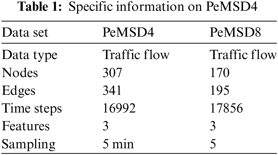
To evaluate the proposed model, many comparative experiments were implemented on the PEMSD4 and PEMSD8 data set for verification. PEMSD4 is data collected from January to February 2018 at 307 monitoring sites in the San Francisco Bay Area, USA. PeMSD8 is the traffic data of San Bernardino from July to August 2016. The data is organized into a record every 5 min and includes data on flow, vehicle speed, and lane occupancy. A specific information summary is in Table 1.

To eliminate the adverse effects of too large or too small traffic volumes on overall predictions in traffic data, This article uses the Z-score side method to standardize the data and all data values fall within the range of [0,1]. The average value is zero.

5.2 Experimental Setup

The mean absolute error (MAE) function and the root mean square error (RMSE) function are used as evaluation functions. MAE can reflect the actual error of the predicted value, while RMSE reflects the square root of the arithmetic mean of the squared error.

The specific formula is defined as

MAE=1m∑i||xi−x^i||(23)

RMSE=1m∑i(Xi−X^)2(24)

The experimental data set is divided into training set, validation set and test set, each with a ratio of 6:2:2. In this paper, 32 1 × 3 convolution kernels are employed in graph convolution and time convolution, the prediction time step c is 12, the learning rate is set to 0.001, the batch size is set to 64, the mean square error is used as the loss function, Adam is used as the optimizer for optimization, and the number of model iterations is set to 100. For each of the three blocks of time and space, we consider 12 historical data: Th = 12, Td = 12, Tw = 12.

5.3 Time Map Threshold Experiment

In this paper, the idea of dynamic programming is used to find the minimum total matching cost recursively. When constructing the temporal graph, a threshold is defined to establish the temporal correlation between nodes. Different threshold values will have a certain impact on the prediction performance of the whole network. Therefore, different temporal maps are established by changing different thresholds for multiple training to verify the best results of the prediction performance of the whole network, as shown in Fig. 7. The optimal prediction can be achieved when the threshold is set to 3200 while the other structures of the whole network remain unchanged.

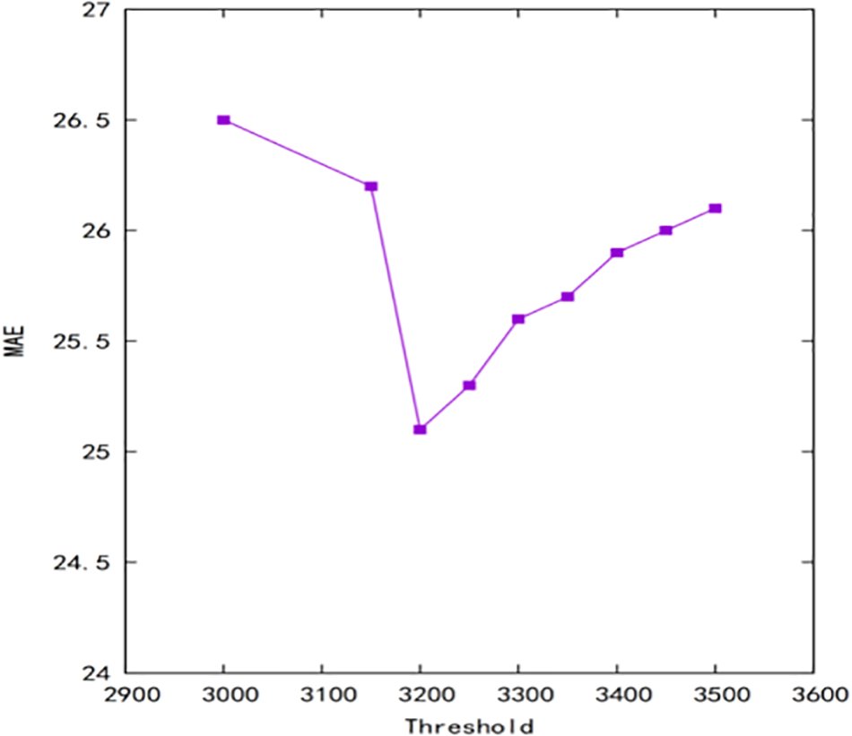
Figure 7: Effect of time graph threshold on MAE

When the threshold is set to 3200, the number of neighboring nodes of each node in the temporal graph must be around five. If the threshold is set too low, the number of adjacent points obtained will be small and the association relationship of the time dimension cannot be effectively extracted. When the setting is large, the number of adjacent nodes is too large, resulting in poor overall prediction.

5.4 Baselines

PyTorch 1.7.2 framework was used to implement the architecture and experimental simulation of the above model. They were trained and evaluated on an NVIDIA GeForce RTX 3090 with 16 GB of memory. Other results refer to ASTGCN [16].

To evaluate the prediction performance of the model proposed in this paper, the following models are selected for comparative analysis.

HA: Predict the traffic value for the next time stamp based on the average traffic flow in the past 1 h.

VAR: The kernel function selected in this article is the radial basis function, with the kernel coefficient set to 0.1.

ARIMA: A classic model for time sequence forecasting analysis, which is simple and does not require other variables.

STGCN: A model based on spatial methods for spatial-temporal data analysis.

ASTGCN: The model fully considers the periodic characteristics of time, and combines graph convolution operation to extract spatial-temporal networks with spatial characteristics.

6  Results and Discussion

We used RMSE and MAE to verify and evaluate the proposed model on the PeMSD4 data set. On average, the model presented in this paper is more effective and efficient than all other comparison models, as shown in Table 2. We analyze in detail the differences between the model presented in this article and other models from three aspects.

6.1 Prediction Accuracy

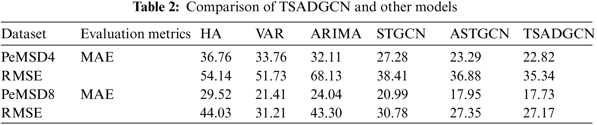
From Table 2, we can see that the proposed TSADGCN model achieves better results in MAE and RMSE in the traffic prediction experiment of 1 h in the future. Compared with HA, VAR increases the nonlinear characteristics of traffic flow information extraction, and ARIMA combines auto-regressive and moving average, the difference between traditional statistical methods, such as to achieve the dependence on traffic flow time series modeling, but can only capture linear relationship, in a complex network structure of traffic flow prediction has great limitations. ASTGCN introduces convolution and attention mechanism, significantly more than ordinary convolution operations comply with the traffic demand forecast. TSADGCN obtains the capture of dynamic spatial-temporal information through attention-based time layers and DGCN. In addition, TSADGCN also considers how to capture deep spatial-temporal features, which helps to achieve better accuracy than these two methods.

6.2 Medium and Long-Term Forecasting Ability

As can be seen from Fig. 8, with the increase in forecast time, the predicted effect of each method presents a different decline. HA and ARIMA methods are very effective for short-term prediction; however, as the prediction time increases, the prediction performance decreases rapidly. Comparing the index parameters of the STGCN, ASTGCN, and TSADGCN proposed in this paper, it can be seen that the effect of TSADGCN is significantly better, and the reason is that STGCN and ASTGCN only considered the proximity in the spatial graph, while TSADGCN constructs the similarity relationship of traffic flow patterns between nodes through the DTW algorithm, establishes the potential traffic flow influence relationship between the nodes of the time graph, and analyzes the structure of the entire road network.

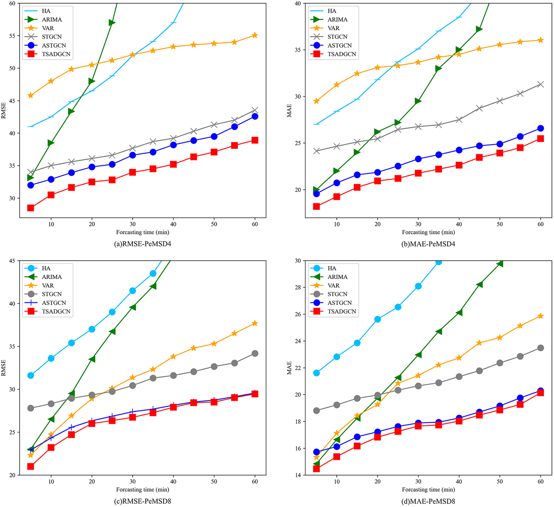
Figure 8: Compared performance for different periods

As can be seen from Fig. 8, the performance of all methods on data set PeMSD4 is worse than that on PeMSD8. Compared with PeMSD8, on the PeMSD4 dataset, the performance improvement among all models is greater. This is because the traffic situation in the PeMSD4 region is more complex and it is more challenging to make predictions using PeMSD4.

Compared with most models, TSADGCN has certain differences in the traffic flow prediction results of different nodes. Table 3 shows the prediction ability of TSADGCN in several nodes, node 137 is the node with the largest error in the whole prediction, and node 196 is the node with the smallest error. Fig. 9 shows the prediction ability of TSADGCN for two traffic flow patterns at three different nodes in total, node 3, node 59, and node 196.

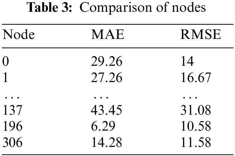
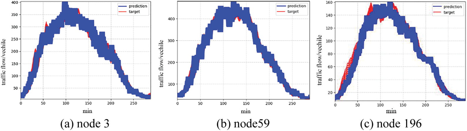
Figure 9: TSADGCN traffic flow prediction graph at different nodes

Combining Table 3 and Fig. 9, we can see that the prediction effect of node 196 is the best among the three nodes. From the prediction of nodes 3, 59, and 196, it can be seen that the more standard the change of traffic data is, the closer the predicted value is to the true value.

Fig. 10 shows the traffic flow prediction results of TSADGCN on node 196 for a week from January 01 to 07, 2018. It can be seen that the model can well track the daily traffic flow changes. This model can effectively capture the time-cycle of the entire traffic change and the spatial-temporal correlation caused by the interaction between different nodes.

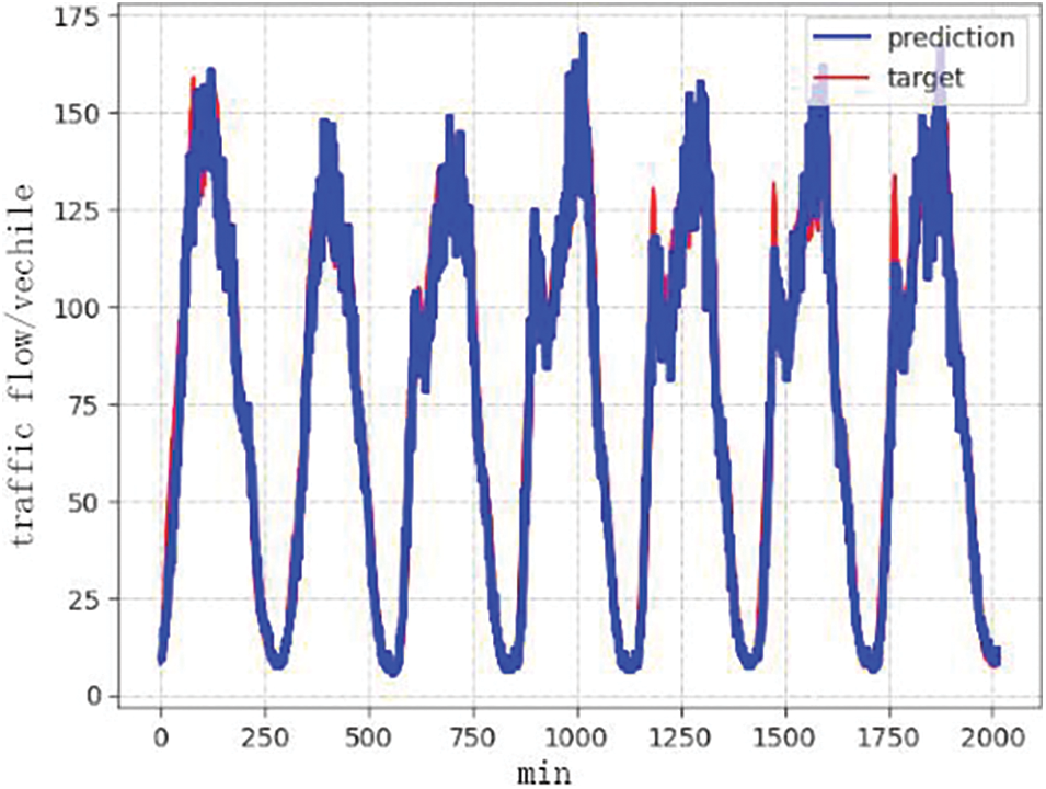
Figure 10: TSADGCN weekly traffic flow forecast at sensor 196

6.3 Ablation Study

To further understand the influence of each module in TSADGCN, ablation comparison experiments are conducted. Based on the TSADGCN model developed in this paper, three variants are designed, as shown below. (1) TSADGCN-T: Remove the TAL module. (2) TSADGCN-R: Remove the residual network. (3) TSADGCN-G: Remove the DGCN module. Fig. 11 shows the prediction error bars of the variant model experiment conducted in the PeMSD4 data set.

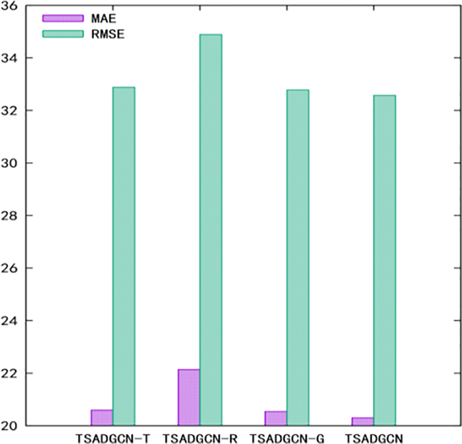
Figure 11: Performance comparison of variant models on the PeMSD4 dataset

It can be seen from Fig. 11 that all modules in the model proposed in this paper can play a role in improving the prediction performance. Among them, the ST graph module has the greatest impact on the model and has a stronger ability to improve the pre-measurement accuracy. The convolution effect of DGCN is second, followed by the residual network. This is because considering the improvement of computational efficiency and prediction effect, the effect of the residual network is not obvious. To sum up, all the modules in the STAGCN model proposed in this paper are effective and can help the model better perform the prediction task.

6.4 Computation Analysis

6.4.1 Computation Time

Table 4 shows the calculation time of TSADGCN, STGCN, and ASTGCN. In this table, we used the PEMD4S dataset to compare the cost of training and inference time for each model. The training time for an epoch is calculated in seconds, while the reasoning time for the entire test data is calculated in seconds. Although TSADGCN takes slightly longer than STGCN and ASTGCN, its predictions are more accurate and efficient. STGCN has the shortest training time. However, its results are poor and less accurate compared to other models.

6.4.2 Complexity Analysis

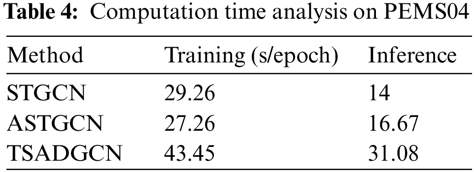
The models presented in this paper are based on time diagrams, spatial diagrams, and space-time diagrams, and add GRU and self-attention layers, which in part increases the complexity of the model. Since each graph processing is independent of each other, the complexity of the model can be reduced.

7  Conclusions and Future Work

This paper proposes TSADGCN, which combines graph convolution network and DGCN to build spatial-temporal convolutional blocks and acquire the spatial-temporal features of traffic data simultaneously. DTW algorithm is used to measure the similarity of time series. Compared with HA, VAR, ARIMA, STGCN, ASTGCN, TSADGCN fully considers the spatial-temporal characteristics of traffic flow and its correlation, and the accuracy of traffic flow prediction is significantly higher than other models. In future work, will further verify the multi-scale information of traffic flow forecasting.

Acknowledgement: The authors would like to express their gratitude for the valuable feedback and suggestions provided by all the anonymous reviewers and the editorial team.

Funding Statement: This work was supported by the National Natural Science Foundation of China (Grant: 62176086).

Author Contributions: Conceptualization, Yunchang Liu; Data curation, Fei Wan; Formal analysis, Yunchang Liu; Methodology, Yunchang Liu and Chengwu Liang; Software, Yunchang Liu and Fei Wan; Writing–original draft, Yunchang Liu and Chengwu Liang. All authors reviewed the results and approved the final version of the manuscript.

Availability of Data and Materials: The training data used in this paper were obtained from the Caltrans performance measurement system. Available online via the following link: https://github.com/divanoresia/Traffic, https://github.com/lyc2688/TSADGCN.

Conflicts of Interest: The authors declare that they have no conflicts of interest to report regarding the present study.

References

1. G. Wei, “A summary of traffic flow forecasting methods,” J. Highway Transp. Res. Dev., vol. 3, pp. 82–85, 2004. [Google Scholar]

2. B. M. Williams and L. A. Hoel, “Modeling and forecasting vehicular traffic flow as a seasonal ARIMA process: Theoretical basis and empirical results,” J. Transp. Eng., vol. 129, no. 6, pp. 664–672, 2003. doi: 10.1061/(ASCE)0733-947X(2003)129:6(664). [Google Scholar] [CrossRef]

3. E. Zivot, “Vector autoregressive models for multivariate time series,” in Modeling Financial Time Series with S-PLUS®, New York, NY: Springer New York, 2006, pp. 385–429. [Google Scholar]

4. I. Okutani and Y. J. Stephanedes, “Dynamic prediction of traffic volume through Kalman filtering theory,” Transp. Res. Part B: Methodol., vol. 18, no. 1, pp. 1–11, 1984. doi: 10.1016/0191-2615(84)90002-X. [Google Scholar] [CrossRef]

5. J. Ye, J. Zhao, K. Ye, and C. Xu, “How to build a graph-based deep learning architecture in traffic domain: A survey,” IEEE Trans. Intell. Transp. Syst., vol. 23, no. 5, pp. 3904–3924, 2022. doi: 10.1109/TITS.2020.3043250. [Google Scholar] [CrossRef]

6. S. Hochreiter and J. Schmidhuber, “Long short-term memory,” Neural Comput., vol. 9, no. 8, pp. 1735–1780, 1997. doi: 10.1162/neco.1997.9.8.1735. [Google Scholar] [PubMed] [CrossRef]

7. J. Chung, C. Gulcehre, K. H. Cho, and Y. Bengio, “Empirical evaluation of gated recurrent neural networks on sequence modeling,” 2014. doi: 10.48550/arXiv.1412.3555. [Google Scholar] [CrossRef]

8. L. Bai, L. Yao, C. Li, X. Wang, and C. Wang, “Adaptive graph convolutional recurrent network for traffic forecasting,” in 34th Int. Conf. Neural Inf. Proc. Syst., Vancouver, BC, Canada, Curran Associates Inc., 2020, pp. 17804–17815. [Google Scholar]

9. S. Yun, M. Jeong, R. Kim, J. Kang, and H. J. Kim, “Graph transformer networks,” 2019. doi: 10.48550/arXiv.1911.06455. [Google Scholar] [CrossRef]

10. M. Li and Z. Zhu, “Spatial-temporal fusion graph neural networks for traffic flow forecasting,” 2020. doi: 10.48550/arXiv.2012.09641. [Google Scholar] [CrossRef]

11. X. Kong, W. Xing, X. Wei, P. Bao, J. Zhang and W. Lu, “STGAT: Spatial-temporal graph attention networks for traffic flow forecasting,” IEEE Access, vol. 8, pp. 134363–134372, 2020. doi: 10.1109/ACCESS.2020.3011186. [Google Scholar] [CrossRef]

12. G. Al-Naymat, S. Chawla, and J. Taheri, “SparseDTW: A novel approach to speed up dynamic time warping,” 2012. doi: 10.48550/arXiv.1201.2969. [Google Scholar] [CrossRef]

13. S. L. Sun, C. S. Zhang, and G. Q. Yu, “A bayesian network approach to traffic flow forecasting,” IEEE Trans. Intell. Transp. Syst., vol. 7, no. 1, pp. 124–132, 2006. doi: 10.1109/TITS.2006.869623. [Google Scholar] [CrossRef]

14. J. Zhang, Y. Zheng, and D. Qi, “Deep spatio-temporal residual networks for citywide crowd flows prediction,” 2016. doi: 10.48550/arXiv.1610.00081. [Google Scholar] [CrossRef]

15. D. Impedovo, V. Dentamaro, G. Pirlo, and L. Sarcinella, “TrafficWave: Generative deep learning architecture for vehicular traffic flow prediction,” Appl. Sci., vol. 9, no. 24, pp. 5504, 2019. doi: 10.3390/app9245504. [Google Scholar] [CrossRef]

16. S. Guo, Y. Lin, N. Feng, C. Song, and H. Wan, “Attention based spatial-temporal graph convolutional networks for traffic flow forecasting,” in 33th AAAI Int. Conf. Artif. Intell., Honolulu, Hawaii, USA, AAAI Press, 2019, pp. 922–929. [Google Scholar]

17. B. Yu, H. Yin, and Z. Zhu, “Spatio-temporal graph convolutional networks: A deep learning framework for traffic forecasting,” 2017. doi: 10.48550/arXiv.1709.04875. [Google Scholar] [CrossRef]

18. C. Zheng, X. Fan, C. Wang, and J. Qi, “GMAN: A graph multi-attention network for traffic prediction,” 2019. doi: 10.48550/arXiv.1911.08415. [Google Scholar] [CrossRef]

19. L. Zhao et al., “T-GCN: A temporal graph convolutional network for traffic prediction,” IEEE Trans. Intell. Transp. Syst., vol. 21, no. 9, pp. 3848–3858, 2020. doi: 10.1109/TITS.2019.2935152. [Google Scholar] [CrossRef]

20. J. Zhu, Q. Wang, C. Tao, H. Deng, L. Zhao and H. Li, “AST-GCN: Attribute-augmented spatiotemporal graph convolutional network for traffic forecasting,” IEEE Access, vol. 9, pp. 35973–35983, 2021. doi: 10.1109/ACCESS.2021.3062114. [Google Scholar] [CrossRef]

21. R. Jain, S. Dhingra, K. Joshi, A. K. Rana, and N. Goyal, “Enhance traffic flow prediction with real-time vehicle data integration,” J. Auton. Intell., vol. 6, no. 2, pp. 574, 2023. doi: 10.32629/jai.v6i2.574. [Google Scholar] [CrossRef]

22. U. K. Lilhore et al., “Design and implementation of an ML and IoT based adaptive traffic-management system for smart cities,” Sens., vol. 22, no. 8, pp. 2908, 2022. doi: 10.3390/s22082908. [Google Scholar] [PubMed] [CrossRef]