TSCND: Temporal Subsequence-Based Convolutional Network with Difference for Time Series Forecasting

1  Introduction

Inferring the future state of data based on past information [1], time series forecasting can help make current decisions, and it has important applications in weather [2], transport [3], finance [4], healthcare [5], and energy [6]. In recent years, research on time series forecasting has evolved from traditional statistical methods and machine learning techniques to forecasting models based on deep learning [7,8].

As a common type of deep learning model for time series modeling, temporal convolutional networks (TCNs) have been widely used in current research on time series forecasting. When dealing with long sequences, TCNs are not as prone to gradient disappearance problems as recurrent neural networks (RNNs). Compared with transformers, TCNs have advantages in memory consumption [9] and do not use the permutation-invariant self-attention mechanism [10], which may lead to temporal information loss. These advantages make TCNs excellent modeling methods for time series forecasting.

Dilated causal convolution plays an important role in TCNs [11], and the structure of dilated causal convolution is shown in Fig. 1. It is essentially a pyramidal-like process of aggregating and learning sequence information. TCNs with dilated causal convolution have excellent memory capabilities [9].

Figure 1: Dilated causal convolution with dilation factors of d = 1, 2, 4 and a filter size of k = 2

However, for time series forecasting, it is unnecessary to employ causal convolution to prevent future information leakage into the past, as the input sequence is solely past information compared to the predicted sequence. Worse still, causal convolution leads to the following problems. On the one hand, in dilated causal convolution, the earlier an input element is located, the greater its effect on the output sequences. For example, in Fig. 1, x1 affects o1,o2,…,ot, while xt only affects the output ot. Nevertheless, the model should focus more on recent elements of the inputs, as recent elements are closer to the time series to be predicted. On the other hand, only the last element ot can receive the information from the whole long sequence, and using this single element instead of a sequence to extract the whole input sequence information may result in serious information loss. Due to the limitations of causal convolution for time series forecasting, we decided to abandon causal convolution and design a new dilated convolution method. Since using a single convolutional filter per layer for dilation convolution tends to lose a lot of information, we use multiple convolutional filters to generate different elements that share the receptive field and form these elements into subsequences. By continuously convolving different subsequences, each final output element can share the receptive field covering the entire input sequence. This is an improvement over the dilated causal convolution in which only the last output element captures the entire input sequence information.

In addition, the problem of distribution shift exists widely in time series, which significantly reduces the performance of forecasting models. The distribution shift problem is that the statistical properties (such as the mean) of the time series may change over time, which may lead to the distribution shift between training and test data. For example, in Fig. 2, there are significant differences in the time series across various time periods. Previous work mainly focused on eliminating discrepancies between the input sequences of the test and training datasets. However, in a long input sequence, the statistical properties vary considerably in different parts of the sequence, thus the discrepancies within an input sequence also need to be addressed. Since differencing can help stabilize the mean of a time series and eliminate trend and seasonality, we use differencing to solve the above problem.

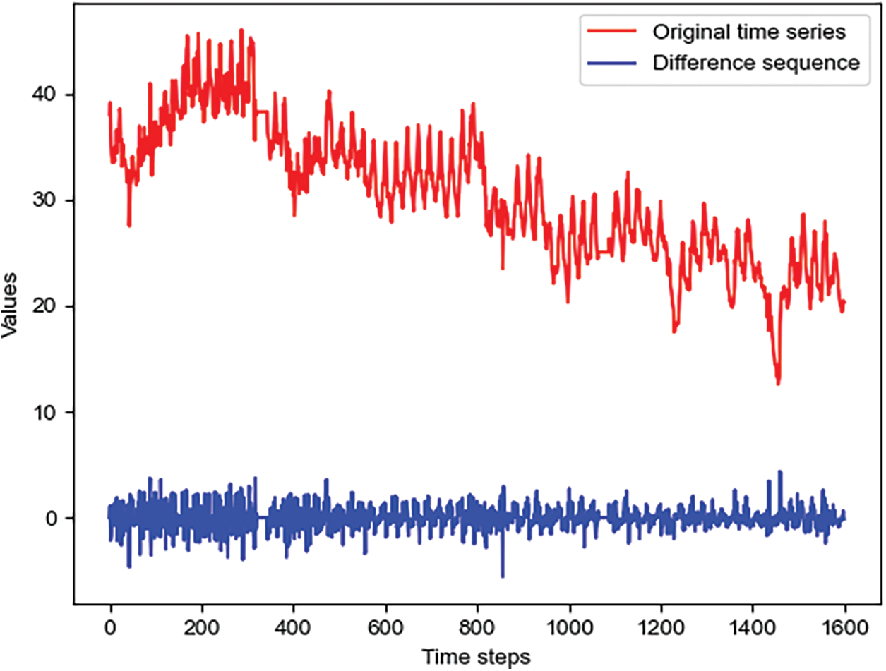
Figure 2: The original time series and difference sequence in the ETTh1 dataset

The contributions of this paper are as follows:

•   To mitigate information loss in dilated convolution on long sequences, we propose a novel subsequence-based convolution method (SDC). The method extracts temporal features from a receptive field via a growing subsequence, and the subsequence has a richer representation than a single element.

•   To break the limitation of dilated causal convolution on the receptive field, we use multiple convolution filters to generate elements that share a receptive field in SDC without causal convolution. As the elements of the shared receptive field increase, eventually, all output elements will be able to look back at the entire input sequence.

•   To alleviate the distribution shift in time series, we propose a difference and compensation method (DCM) to reduce the discrepancies between and within input sequences by difference operations. As shown in Fig. 2, difference operation greatly reduces the variance of sequences at different time periods.

•   Based on SDC and DCM, we further construct a temporal subsequence-based convolutional network with difference (TSCND) for time series forecasting. Experimentally, compared with state-of-the-art methods and vanilla TCN, TSCND can reduce prediction mean squared error by 7.3% and save runtime. The results of the ablation experiments also demonstrate the effectiveness of SDC and DCM for time series forecasting.

2  Related Works

2.1 Time Series Forecasting

Current time series forecasting methods can be divided into traditional statistics-based methods and deep learning-based methods.

Traditional statistics-based methods, such as the autoregressive integrated moving average (ARIMA) [12] and Kalman filter models [13], have had extensive theoretical research in the past. However, these traditional statistical-based methods perform poorly on complex time series.

Deep learning can automatically learn and model the hidden features of complex series based on raw data and can achieve better forecasting accuracy on complex time series datasets. Therefore, more research is now based on deep learning methods.

Recurrent neural networks (RNNs) [14] play an important role in time series forecasting [15–17]. However, when the given time series is long, much of the information contained earlier in the time series will be lost [18].

In recent years, transformer-based models [19] have been widely used for time series forecasting tasks [20]. Informer [21] reduces the computational complexity of the self-attention mechanism and performs well in long-term time series forecasting. Autoformer [22] uses autocorrelation attention and seasonal decomposition methods for model construction, reducing the required computational workload and improving forecasting accuracy. FEDformer [23] uses the seasonal trend decomposition method and frequency-enhanced attention. PatchTST [24] achieves SOTA accuracy on several long-term time series forecasting datasets based on channel independence and subseries-level patch input mechanism. However, when these transformer-based models deal with long sequence data, they always require considerable computational resources and memory. In addition, using self-attention mechanisms for time series modeling may lead to the loss of temporal information [10].

TCNs are also popular for time series forecasting tasks [25–28]. MISO-TCN [29] is a lightweight and novel weather forecasting model based on TCN. TCN-CBAM [30] uses the convolutional block attention module for the prediction of chaotic time series. VMD-GRU-TCN [31] integrates variational modal decomposition, gated recurrent unit and TCN into a hybrid network for high and low frequency load forecasting. Veg-W2TCN [32] combines multi-resolution analysis wavelet transform and TCN for vegetation change forecasting. TCNs use dilated causal convolution in the temporal dimension to learn temporal dependencies [33,34]. For vanilla convolution operations, the size of the receptive field is linearly related to the number of convolution layers, which leads to an inability to handle long sequence inputs. Dilated causal convolution is a very efficient structure that helps a model achieve exponential receptive field sizes. For an input sequence X={x0,x1,…,xt}, the dilated causal convolution operation for the element located at s can be formalized as:

F(s)=∑i=0k−1f(i)⋅xs−di(1)

where fn:{0,…,k−1}→R is a convolutional filter, d is the dilation factor, and k is the convolutional filter size. The use of a larger d allows the top output to represent a larger range of inputs, which effectively expands the receptive field of the convolutional network, as shown in Fig. 1.

Dilated causal convolution can capture the long-term dependencies of the time series, but the causal convolution structure limits the receptive field and results in severe information loss during dilated convolution. Therefore, we propose a new dilated convolution method to replace dilated causal convolution in TCNs.

2.2 Distribution Shift Problem Addressing

Forecasting models often suffer badly from distribution shift in time series. Domain adaptation [35] and domain generalization [36] are common methods to alleviate the distribution shift [37,38]. However, these methods are often complex, and it is not easy to define the domain in non-stationary time series. Recently, some simple and effective methods have been proposed to address the distribution shift problem. The Revin method [39] normalizes each input sequence and then non-normalizes the model output sequence. However, this method prevents the model from obtaining features such as the magnitude of data changes. The NLinear model [10] uses a method of subtracting the end value of the input sequence from each value of the input sequence and restoring the end value to the output sequence. However, there is a problem of significant differences within the input sequence, which undermines the effectiveness of model training. Our proposed method minimizes the difference between and within input sequences without losing information in the original data.

3  Methods

3.1 Model Structure

The overall architecture of our proposed model is shown in Fig. 3. First, the DCM carries out a difference operation on the input time series to obtain difference sequences with smaller discrepancies in values, and then the Padding operation is used to extend the sequence length to meet the requirements of dilated convolution. Next, the Embedding operation maps the padded sequences to a high-dimensional space, followed by multiple layers of SDC to extract temporal dependencies of the input. Finally, the Decoding operation is used and the DCM restores the original input values to the Decoding output to obtain the prediction result.

Figure 3: Overview of the TSCND architecture

3.2 Difference and Compensation Method (DCM)

DCM is used to address the problem of distribution shift. It contains a difference stage and a compensation stage.

In the difference stage, a difference sequence is obtained through differencing adjacent elements in an input sequence. For an input sequence X={x0,x1,…,xt} with length t, the difference stage can be formalized as:

Xd={x1−x0,x2−x1,…,xt−xt−1}(2)

In the compensation stage, to compensate for the information loss caused by difference operation, the last element value of the original sequence is added back to the output. For the output sequence Y={y0,y1,…,yq} of length q, the compensation stage can be formalized as:

Y={y0+xt,y1+xt,…,yq−1+xt,yq+xt}(3)

3.3 Padding and Embedding

To ensure that the sequence length can meet the requirements of the SDC, we pad the difference sequence Xd with zeros, and the length L of the padded sequence is:

L=kc(4)

where k is the convolutional filter size, and c is the number of layers of the Muti-layer SDC.

The process of padding and embedding the sequence Xd can be formalized as:

Xp=Padding(Xd),(5)

H0=Embedding(Xp)(6)

where Embedding(.) is a linear layer that maps the padded sequence Xp∈Rvar×L to H0∈Rdim×L, var denotes the number of variates in time series, dim is a hyperparameter that represents the hidden variable dimension of the model, H0 is the input of Muti-layer SDC.

3.4 Subsequence-Based Dilated Convolution Layer

Due to the limitation of dilated causal convolution on the receptive field, we propose the SDC to be used instead of dilated causal convolution. Our SDC has the following two similarities with dilated causal convolution: (1) The size of the receptive field of the output sequence elements is exponentially related to the number of network layers, so very large receptive fields can be achieved by stacking a few convolutional layers. (2) The input and output sequences are of equal length, which facilitates the stacking of layers to obtain a larger receptive field. The uniqueness of SDC is that it uses multiple convolutional filters to convolve the elements of adjacent subsequences. The elements in a subsequence share a receptive field. Fig. 4 shows a 3-layer SDC structure.

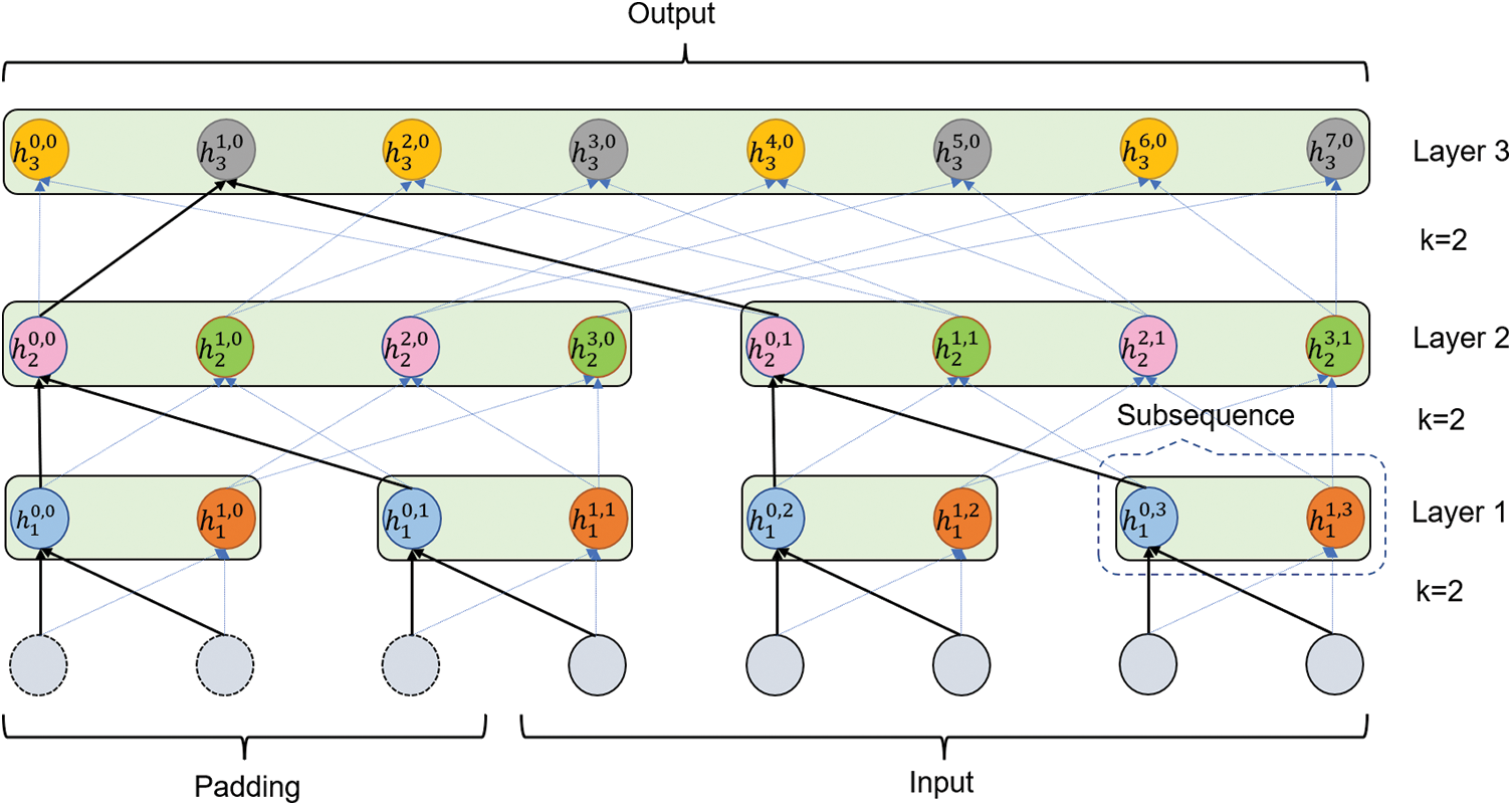
Figure 4: The multi-layer SDC contains 3 SDC layers with k (here k=2) convolution filters at each layer, this figure omits the residual connection. The elements generated using the same convolution filter are represented by the same color (e.g., at Layer 2, the elements colored in red are all generated by the same convolution filter, but they do not share a convolution filter with the green elements). Subsequences are marked by rounded rectangles in the figure. Solid lines show how an output element acquires information about the entire input sequence via the SDC

At the SDC layer, an input or output sequence is divided into several subsequences. For multi-layer SDC, the initial subsequence length is 1, and the length will increase with the number of SDC layers by SDC operation. Each SDC layer uses k convolutional filters of size k, which means that the size and number of convolutional filters used in each layer are equal. This setting ensures that the input and output sequences possess equal lengths.

Specifically, at SDC Layer i, k input subsequences are convolved to generate an output subsequence whose length is the sum of the lengths of these input subsequences. Therefore, we can calculate the length of subsequences for each layer. The output sequence Hi of SDC Layer i can be expressed based on subsequence as:

Hi={hi0,0,…,hia,b,…,hiri−1,pi−1}(7)

where hia,b denotes the a-th element of the b-th subsequence, the subsequence length ri=ki, ki is the i-th power of k, pi is the number of the subsequences, and pi=L/ri.

The detailed process of the SDC operation for convolving subsequences is as follows: firstly, the elements in the neighboring subsequences are convolved using several different filters, and elements in the same subsequence are not convolved with each other. Then the output elements generated by convolving the same elements but with different convolution filters are adjacent to each other, and the elements generated by the same subsequences are merged into a new subsequence. E.g., in Fig. 4, convolution between h10,0 and h10,1, not between h10,0 and h11,0, the output elements h20,0 and h21,0 generated by the same input elements are adjacent to each other.

We first formalize SDC operations from the perspective of a single output element. The SDC operation on the a-th element h^ia,b of the b-th subsequence can be formalized as:

h^ia,b=fdc(Hi−1,a,b)=∑n=0k−1fm(n)⋅hi−1r.,p.+n(8)

where Hi−1 is the input sequence of Layer i, k is the convolutional filter size, fm:{0,…,k−1}→R is the m-th convolution filter, m=amodk, r.=⌊ak⌋, and p.=b⋅k.

Next, based on the SDC operation for a single element, we extend to the SDC operation for the sequence. The SDC operation for the input sequence Hi−1 can be formalized as:

H^i=FDC(Hi−1)(9)

={h^i0,0,…,h^iri−1,pi−1}

={fdc(Hi−1,0,0),…,fdc(Hi−1,ri−1,pi−1)}

For a SDC Layer i, the output Hi is obtained after SDC operation and residual connection, the process can be formalized as:

Hi=ReLU(H^i+Hi−1)(10)

where ReLU(⋅) is the rectified linear unit (ReLU) activation function [40].

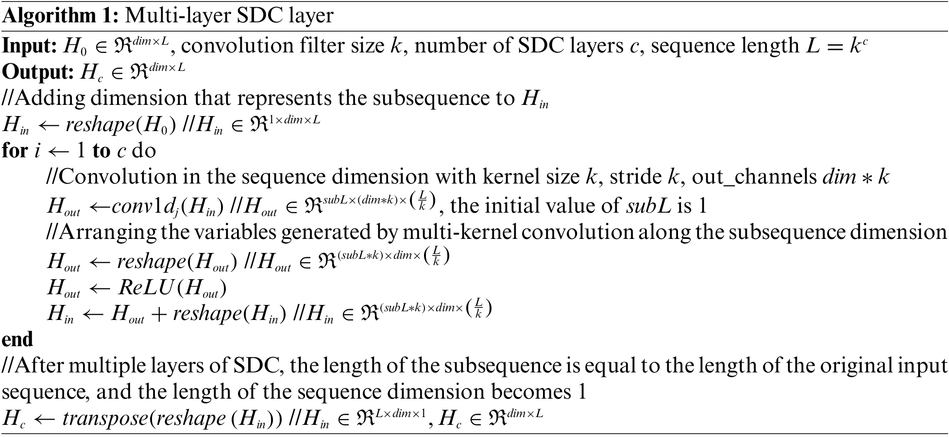
To enhance the comprehensibility of the SDC layer, we utilize pseudo-code to illustrate the process in Algorithm 1.

3.5 Decoding

The Decoding module includes 2 fully-connected layers. The one maps Hc∈Rdim×L to Hd∈Rtvar×L, tvar denotes the number of target variates to be predicted. And then the other one maps Hd∈Rtvar×L to Y ∈Rtvar×pL, pL denotes the time step of the target variates.

4  Experiments

To evaluate our model’s performance, we conducted univariate time series forecasting on four popular real-world datasets ETTh1, ETTh2, ECL, and WTH.

4.1 Datasets

ETT (Electricity Transformer Temperature): This dataset consists of the electricity transformer temperature derived from two different countries in China for two years. ETTh1 and ETTh2 correspond to data collected at one-hour intervals from these two counties. The target “oil temperature” was predicted based on past data. The train/val/test is 12/4/4 months.

ECL (Electricity Consumption Load): This dataset collects the electricity consumption loads (kWh) of 321 customers. We set “MT_320” as the target value. The training, validation, and test sets were scaled to 0.6/0.2/0.2.

WTH (Weather): This dataset collects four years of climate data from 2010 to 2013; it covers 1600 locations in the United States, with data points collected every hour. Each data point consists of the target value “wet bulb”. The training, validation, and test sets were scaled to 0.6/0.2/0.2.

4.2 Baselines

To verify the superiority of our proposed method, we compared it with four SOTA models: PatchTST, FEDformer, Autoformer, and Informer. In addition, our proposed method was also compared with the classic models TCN and LSTM.

PatchTST (2023) [24]: This is a transformer-based model. it achieves SOTA accuracy on ETTh1 and ETTh2 datasets based on channel independence and subseries-level patch input mechanism.

FEDformer (2022) [23]: This is a transformer-based model. It uses the seasonal trend decomposition method and a frequency-enhanced attention module. Since the frequency-enhanced attention module has linear complexity, FEDformer is more efficient than the standard transformer. It achieves the best forecasting performance on the benchmark dataset in comparison with previous state-of-the-art algorithms.

Autoformer (2021) [22]: This is a transformer-based model. It uses auto-correlation attention and seasonal decomposition for model construction, reducing the required computational effort and achieving improved forecasting accuracy.

Informer (2021) [21]: This is an efficient transformer-based model that uses the ProbSparse self-attention mechanism to reduce its computational complexity. The model performs well in long-term time series prediction tasks.

TCN (2018) [9]: This is a convolutional network for sequence modeling that uses dilated causal convolution. It outperforms recurrent neural networks in many sequence modeling tasks.

LSTM (1997) [41]: This is a recurrent neural network whose gating mechanism alleviates the problem of gradient disappearance and allows the model to capture long-term dependencies.

4.3 Evaluation Metrics

We used the following evaluation metrics:

(1) Mean squared error (MSE):

MSE=1n∑(y−y∗)2(11)

(2) Mean absolute error (MAE):

MAE=1n∑|y−y∗|(12)

where n is the number of time steps to be predicted, y is the predicted value, and y∗ is the ground truth.

4.4 Implementation Details

For all the compared models, the same parameter settings were used for the training process, with predicted sequence lengths of 24, 48, 168, 336, and 720. The models were optimized using the adaptive moment estimation (Adam) optimizer with learning rates starting at 1e-3. The total number of epochs is 8 with proper early stopping. We used Mean Squared Error (MSE) as our loss function. The inputs of each dataset were zero-mean normalized. Following the previous related work [42], we used a 10-residual-block stack in the TCN. Referring to Informer [21] and PatchTST [24], the input length was selected from {168, 336, 512, 720}. The other settings used their default values.

For better performance of TSCND, we set the convolutional filter size k to 2 and the hidden layer dimension dim to 64 based on the validation dataset. To allow the output elements to have a look back at the entire input sequence while the model has as little computational effort as possible, the number of model layers is computed from the input length t, and the number of model layers c=⌊logk⁡t⌋+1.

4.5 Experimental Results

Tables 1 and 2 list the forecasting results of the comparison models and our model. Our model achieved the best results in 32/40 cases and the second-best results in 6/8 cases where it did not achieve the best results. Compared with the SOTA model PatchTST, our model yields an overall 7.3% relative MSE reduction, and when the prediction length is 720, the improvement can be more than 15%. TSCND performs slightly worse than PatchTST on the MSE metrics in the ETTh1 dataset. This is due to the presence of many outliers in the ETTh1 dataset, and the self-attention mechanism employed by PatchTST is more advantageous than convolutional networks in dealing with outliers. Meanwhile, TSCND outperforms PatchTST on the MAE metric in the ETTh1 dataset. This metric is insensitive to outliers, which supports the above view and suggests that TSCND is better at predicting the normal value of ETTh1.

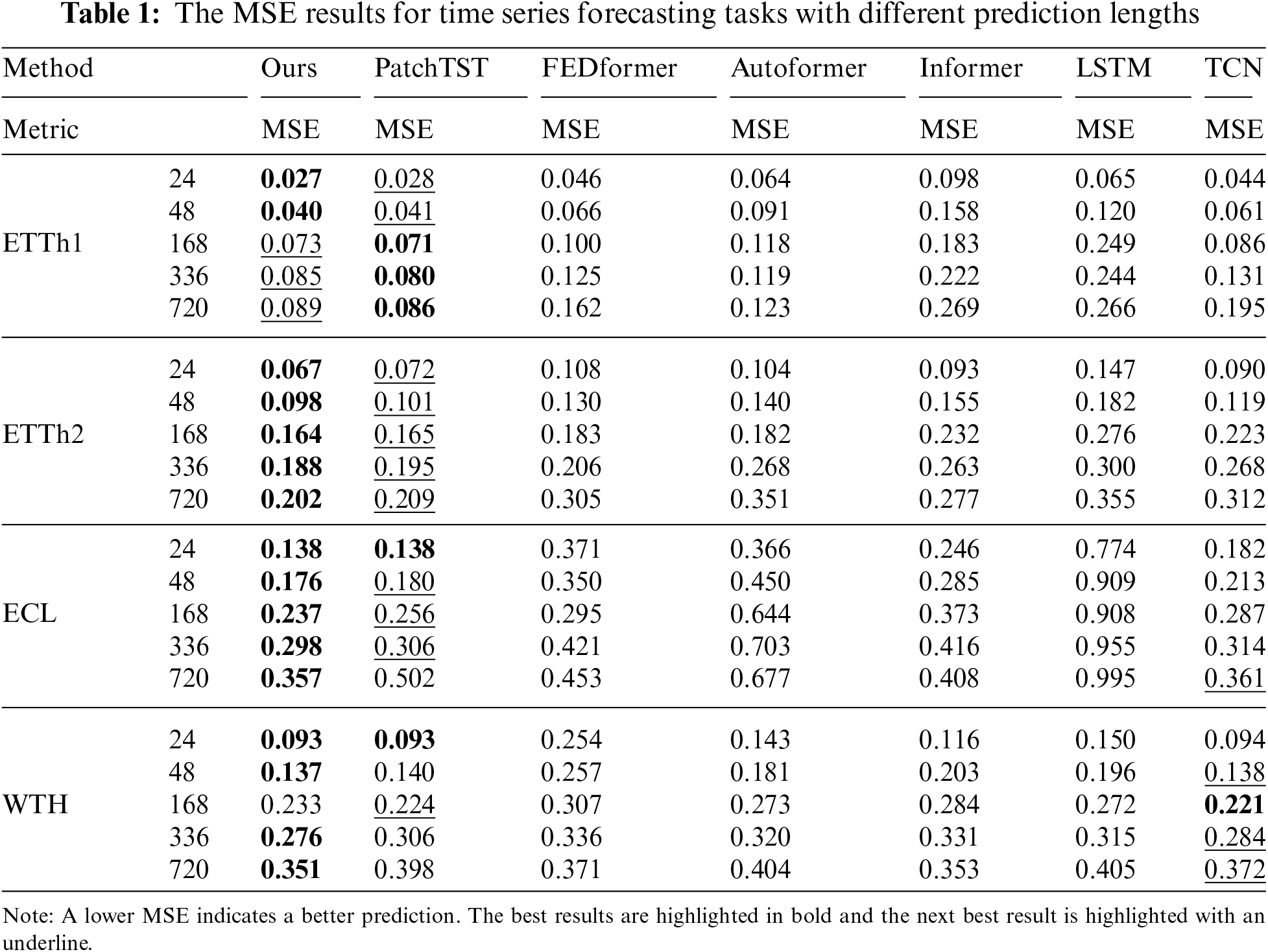
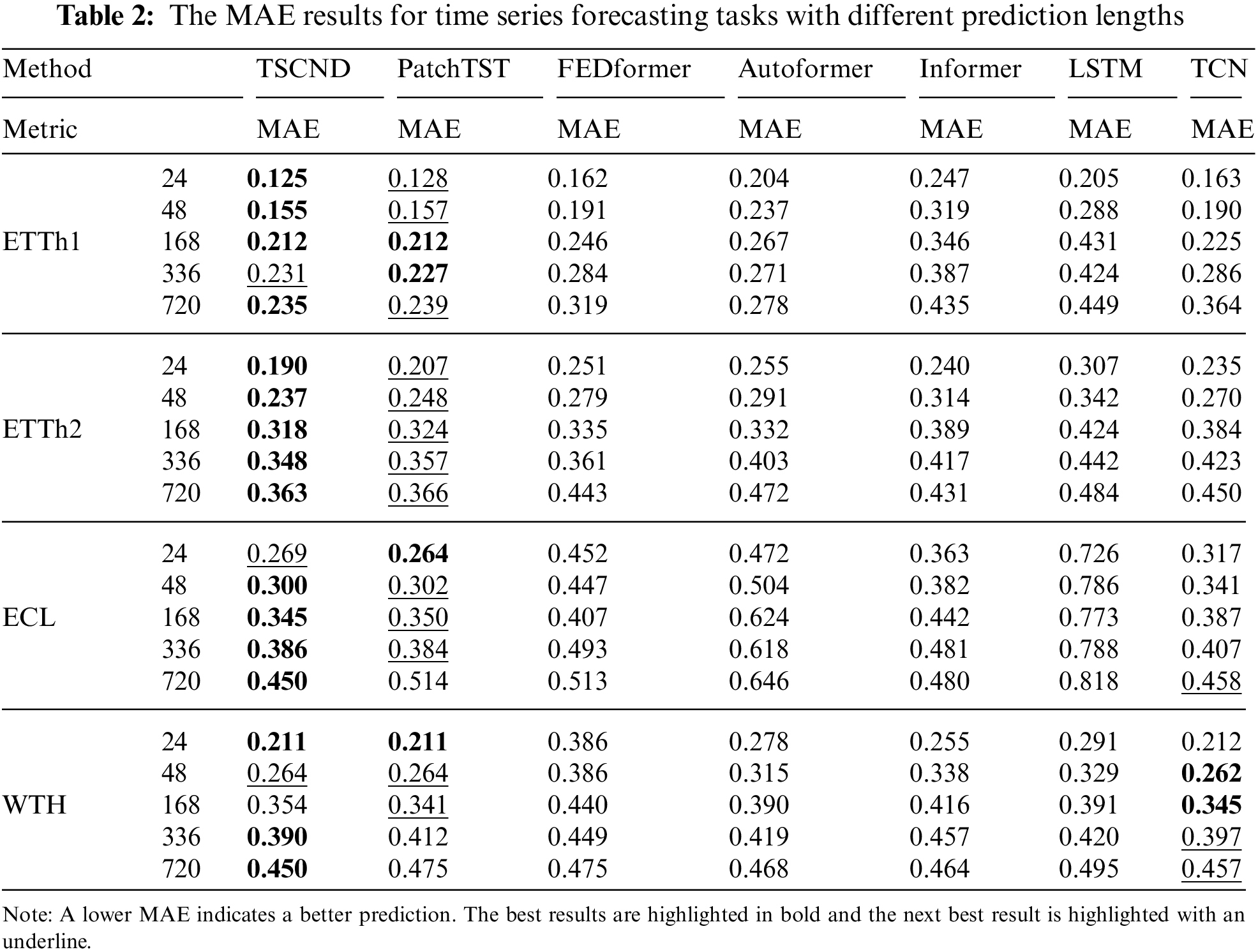
Compared to TCN, our method brings improvement in all cases on ETTh1, ETTh2, and ECL datasets, and brings improvement in 7/10 cases on WHT datasets. It achieved better results than TCN, with an average MSE reduction of 19.4%. In the short-term forecasting of WTH, the results of TSCND and TCN are similar for the following reasons. The time series of the WTH dataset is relatively stationary, thus the DCM method is of little help to the model. And when the prediction length is short, this advantage of SDC using subsequences instead of elements to extract features is not obvious, so TSCND and TCN perform similarly. However, when predicting long-term time series, TSCND is superior to TCN.

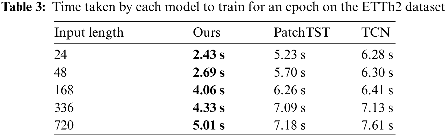
To evaluate the efficiency of our proposed model in handling inputs of different lengths, we chose PatchTST and TCN for comparison. We compared the time required for training each model for 1 epoch on the ETTh2 dataset under different input sequence lengths. The results are shown in Table 3. Compared with PatchTST and TCN, it reduces training time by over 40% on average. The reason for the faster training speed of TSCND compared to TCN is that (1) TSCND uses only one convolutional layer per layer, while TCN uses two convolutional layers per layer. (2) TSCND is designed with the number of layers adjusted according to the length of the inputs, while TCN has a fixed number of layers. TSCND uses fewer layers when processing short inputs. (3) Since the stride length of the convolutional layers in TCN is shorter than in TSCND, the elements of each layer in TCN participate in the convolution more times.

4.6 Ablation Studies

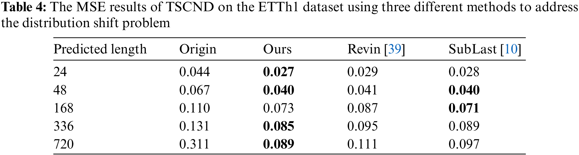
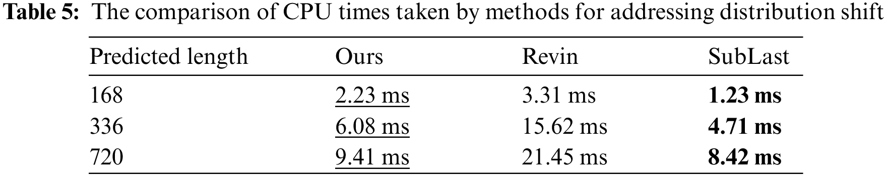
To evaluate the proposed method for addressing the distribution shift problem, we conducted experiments on the ETTh1 dataset using our proposed method, the Revin method (Revin) [39], and the NLinear method (SubLast) [10]. The experimental results are shown in Table 4, and it can be seen that our method achieves the best performance in almost all cases. Compared with the original input, our method yields an overall 52.6% relative MSE reduction, indicating the effectiveness of the proposed method. We conducted experiments using CPU AMD Ryzen 7 5800 to compare the time taken by our method with the other methods. The results of CPU times are shown in Table 5. Our method takes more time than the SubLast method but much less time than the Revin method. This time is almost negligible compared to the overall training time of the model. Therefore, we believe that our method remains an alternative to SubLast method where efficiency is pursued.

To test whether a subsequence can capture more temporal dependencies than a single element, we tested three different structures of the Decoder Layer for making predictions using SDC output.

Structure A: This is also the structure as that in TSCND. The structure uses the whole output sequence to predict each future time point, which is shown as Structure A in Fig. 5.

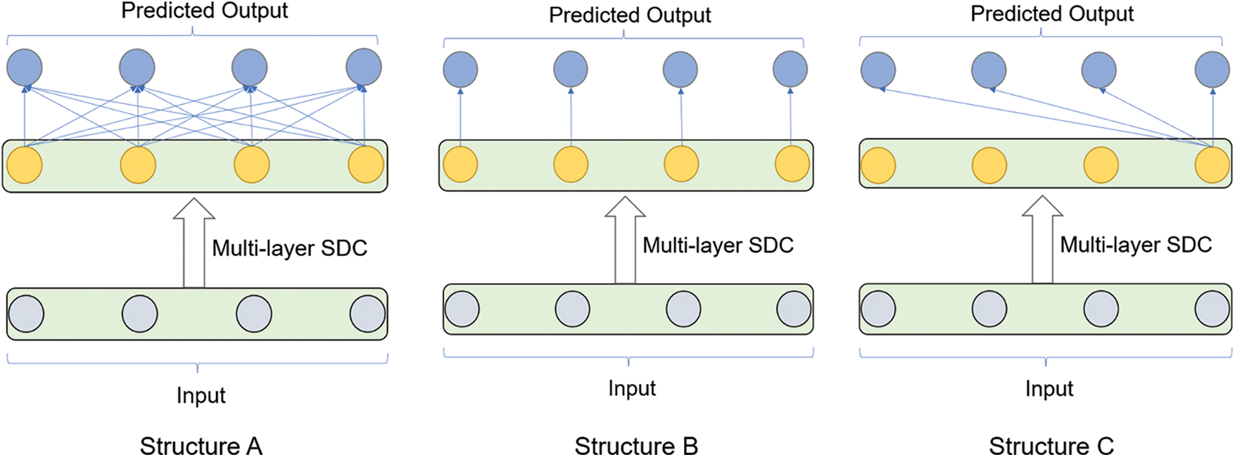
Figure 5: Three different decoding structures

Structure B: In this structure, each single output element of the Multi-layer SDC is used to predict a time point independently, which is shown as Structure B in Fig. 5.

Structure C: This is similar to the dilated causal convolution, where only one output element can obtain information about the whole input sequence. The structure predicts each time point using a single element of the Multi-layer SDC outputs, which is shown as Structure C in Fig. 5.

We conducted experiments using above structures on the ECL dataset, and the experimental results are shown in Fig. 6. The prediction error of Structure A is much lower than the other two structures under all lengths, especially for long lengths. Using output sequences rather than single elements for prediction improves prediction accuracy, indicating that SDC can enhance feature extraction by using subsequences to extract features from receptive fields.

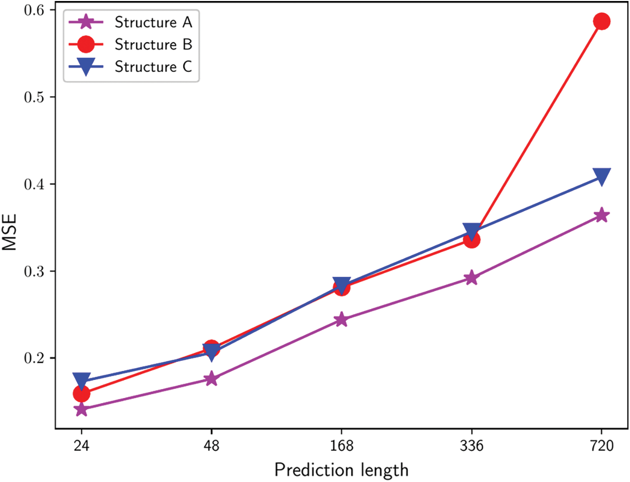
Figure 6: Time series forecasting results of three different decoding structures on the ECL dataset

5  Conclusions

This paper proposes a temporal subsequence-based convolutional network with difference for time series forecasting, with two effective modules: (i) SDC, which extracts information from a receptive field via a subsequence rather than a single element, and multiple convolutional filters are used at each layer to enable the elements in the same subsequence to share a receptive field. These designs allow the receptive fields of all final output elements to cover the entire input sequence, thus reducing the loss of information in the dilated convolution. (ii) DCM, which can effectively solve the problem of distribution shift. The method reduces the discrepancies between and within input sequences through difference operations. By restoring the original input information to the outputs, the method can compensate for the loss of information due to difference operations.

We conducted experiments on commonly used time series datasets. Firstly, TSCND outperforms the SOTA method on most of the MAE and MSE metrics, which indicates that TSCND is effective in both short-term and long-term time series forecasting. Secondly, the experiments on training time demonstrate the advantage of TSCND in efficiency. Finally, ablation experiments show that DCM is useful in mitigating the distribution shift problem and the use of subsequences instead of single elements in the SDC method can enhance the feature extraction capability.

In future work, we will further study from the following directions: Firstly, the convolution filter size and hidden layer dimension of the proposed model are important hyperparameters. They are currently set manually relying on experience, and it would be valuable to study the automatic selection of these hyperparameters. Then we will explore combining the proposed SDC with research on heterogeneous information systems for multivariate time series forecasting. Finally, we will consider the possibility of the SDC as an alternative to dilated causal convolution for time series classification and anomaly detection.

Acknowledgement: We thank the members of the MOE Research Center of Software/Hardware Co-Design Engineering for their contributions to this work.

Funding Statement: This work was supported by the National Key Research and Development Program of China (No. 2018YFB2101300), the National Natural Science Foundation of China (Grant No. 61871186), and the Dean’s Fund of Engineering Research Center of Software/Hardware Co-Design Technology and Application, Ministry of Education (East China Normal University).

Author Contributions: The authors confirm contribution to the paper as follows: study conception and design: Haoran Huang and Weiting Chen; data collection: Haoran Huang; analysis and interpretation of results: Haoran Huang and Weiting Chen; draft manuscript preparation: Haoran Huang, Weiting Chen, and Zheming Fan. All authors reviewed the results and approved the final version of the manuscript.

Availability of Data and Materials: All datasets that support the findings of this study are openly available. The ETT dataset is available at https://github.com/zhouhaoyi/ETDataset; The ECL dataset is available at https://archive.ics.uci.edu/ml/datasets/ElectricityLoadDiagrams20112014; The WTH dataset is available at https://www.ncei.noaa.gov/data/local-climatological-data/. The code repository address of this paper is https://github.com/1546645614/TSCND.

Conflicts of Interest: The authors declare that they have no conflicts of interest to report regarding the present study.

References

1. X. H. Wang, Y. Wang, J. J. Peng, Z. C. Zhang, and X. L. Tang, “A hybrid framework for multivariate long-sequence time series forecasting,” Appl. Intell., vol. 53, no. 11, pp. 13549–13568, 2023. doi: 10.1007/s10489-022-04110-1. [Google Scholar] [CrossRef]

2. M. Fathi, K. M. Haghi, S. M. Jameii, and E. Mahdipour, “Big data analytics in weather forecasting: A systematic review,” Arch. Comput. Method. Eng., vol. 29, no. 2, pp. 1247–1275, 2022. doi: 10.1007/s11831-021-09616-4. [Google Scholar] [CrossRef]

3. Y. H. Wang, S. Fang, C. X. Zhang, S. M. Xiang, and C. H. Pan, “TVGCN: Time-variant graph convolutional network for traffic forecasting,” Neurocomputing, vol. 471, no. 6, pp. 118–129, 2022. doi: 10.1016/j.neucom.2021.11.006. [Google Scholar] [CrossRef]

4. P. D’Urso, L. de Giovanni, and R. Massari, “Trimmed fuzzy clustering of financial time series based on dynamic time warping,” Ann. Oper. Res., vol. 299, pp. 1379–1395, 2021. doi: 10.1007/s10479-019-03284-1. [Google Scholar] [CrossRef]

5. F. Piccialli, F. Giampaolo, E. Prezioso, D. Camacho, and G. Acampora, “Artificial intelligence and healthcare: Forecasting of medical bookings through multi-source time-series fusion,” Inf. Fusion, vol. 74, no. 1, pp. 1–16, 2021. doi: 10.1016/j.inffus.2021.03.004. [Google Scholar] [CrossRef]

6. J. Z. Zhu, H. J. Dong, W. Y. Zheng, S. L. Li, Y. T. Huang and L. Xi, “Review and prospect of data-driven techniques for load forecasting in integrated energy systems,” Appl. Energ., vol. 321, pp. 119269, 2022. doi: 10.1016/j.apenergy.2022.119269. [Google Scholar] [CrossRef]

7. C. R. Yin and D. Qun, “A deep multivariate time series multistep forecasting network,” Appl. Intell., vol. 52, no. 8, pp. 8956–8974, 2022. doi: 10.1007/s10489-021-02899-x. [Google Scholar] [CrossRef]

8. W. F. Liu, X. Yu, Q. Y. Zhao, G. Cheng, X. B. Hou and S. Q. He, “Time series forecasting fusion network model based on prophet and improved LSTM,” Comput. Mater. Contin., vol. 74, no. 2, pp. 3199–3219, 2023. doi: 10.32604/cmc.2023.032595. [Google Scholar] [PubMed] [CrossRef]

9. S. J. Bai, J. Z. Kolter, and Y. Koltun, “An Empirical evaluation of generic convolutional and recurrent networks for sequence modeling,” arXiv preprint arXiv:1803.01271, 2018. [Google Scholar]

10. A. L. Zeng, M. X. Chen, L. Zhang, and Q. Xu, “Are transformers effective for time series forecasting?,” in Proc. AAAI Conf. Artif. Intell., Washington, USA, 2023, vol. 37, pp. 11121–11128. [Google Scholar]

11. M. H. Liu et al., “Scinet: Time series modeling and forecasting with sample convolution and interaction,” in Proc. Annu. Conf. Neural Inform. Process. Syst., New Orleans, USA, 2022, vol. 35, pp. 5816–5828. [Google Scholar]

12. G. E. Box and G. M. Jenkins, “Some recent advances in forecasting and control,” J. R. Stat. Soc. Ser. C. (Appl. Stat.), vol. 17, no. 2, pp. 91–109, 1968. doi: 10.2307/2985674. [Google Scholar] [CrossRef]

13. G. W. Morrison and D. H. Pike, “Kalman filtering applied to statistical forecasting,” Manage. Sci., vol. 23, no. 7, pp. 768–774, 1977. [Google Scholar]

14. K. Greff, R. K. Srivastava, J. Koutník, B. R. Steunebrink, and J. Schmidhuber, “LSTM: A search space odyssey,” IEEE Trans. Neur. Net. Lear. Syst., vol. 28, no. 10, pp. 2222–2232, 2016. doi: 10.1109/TNNLS.2016.2582924. [Google Scholar] [PubMed] [CrossRef]

15. D. Salinas, V. Flunkert, J. Gasthaus, and T. Januschowski, “DeepAR: Probabilistic forecasting with autoregressive recurrent networks,” Int. J. Forecasting, vol. 36, no. 3, pp. 1181–1191, 2020. doi: 10.1016/j.ijforecast.2019.07.001. [Google Scholar] [CrossRef]

16. X. Gao, X. B. Li, B. Zhao, W. J. Ji, X. Jing and Y. He, “Short-term electricity load forecasting model based on EMD-GRU with feature selection,” Energies, vol. 12, no. 6, pp. 1140, 2019. doi: 10.3390/en12061140. [Google Scholar] [CrossRef]

17. J. Wang, J. X. Cao, S. Yuan, and M. Cheng, “Short-term forecasting of natural gas prices by using a novel hybrid method based on a combination of the CEEMDAN-SE-and the PSO-ALS-optimized GRU network,” Energy, vol. 233, no. 10, pp. 121082, 2021. doi: 10.1016/j.energy.2021.121082. [Google Scholar] [CrossRef]

18. Q. L. Ma, Z. X. Lin, E. H. Chen, and G. Cottrell, “Temporal pyramid recurrent neural network,” in Proc. AAAI Conf. Artif. Intell., New York, USA, 2020, vol. 34, no. 1, pp. 5061–5068. doi: 10.1609/aaai.v34i04.5947. [Google Scholar] [CrossRef]

19. A. Vaswani et al., “Attention is all you need,” in Proc. Annu. Conf. Neural Inform. Process. Syst., California, USA, 2017, vol. 30. [Google Scholar]

20. M. Zaheer et al., “Big bird: Transformers for longer sequences,” in Proc. Annu. Conf. Neural Inform. Process. Syst., 2020, vol. 33, pp. 17283–17297. [Google Scholar]

21. H. Y. Zhou et al., “Informer: Beyond efficient transformer for long sequence time-series forecasting,” in Proc. AAAI. Conf. Artif. Intell., 2021, vol. 35, pp. 11106–11115. doi: 10.1609/aaai.v35i12.17325. [Google Scholar] [CrossRef]

22. H. X. Wu, J. H. Xu, J. M. Wang, and M. S. Long, “Autoformer: Decomposition transformers with auto-correlation for long-term series forecasting,” in Proc. Annu. Conf. Neural Inform. Process. Syst., Montreal, Canada, 2021, vol. 34, pp. 22419–22430. [Google Scholar]

23. T. Zhou, Z. Q. Ma, Q. S. Wen, X. Wang, L. Sun and R. Jin, “FEDformer: Frequency enhanced decomposed transformer for long-term series forecasting,” in Proc. Int. Conf. Mach. Learn., Maryland, USA, 2022, pp. 27268–27286. [Google Scholar]

24. Y. Nie, N. H. Nguyen, P. Sinthong, and J. Kalagnanam, “A time series is worth 64 words: Long-term forecasting with transformers,” in Proc. Int. Conf. Learn. Representations, Kigali, Rwanda, 2023, pp. 1–25. [Google Scholar]

25. J. F. Torres, D. Hadjout, A. Sebaa, F. Martínez-Álvarez, and A. Troncoso, “Deep learning for time series forecasting: A survey,” Big Data, vol. 9, no. 1, pp. 3–21, 2021. doi: 10.1089/big.2020.0159. [Google Scholar] [PubMed] [CrossRef]

26. C. Guo, X. M. Kang, J. P. Xiong, and J. H. Wu, “A new time series forecasting model based on complete ensemble empirical mode decomposition with adaptive noise and temporal convolutional network,” Neural Process. Lett., vol. 55, no. 4, pp. 4397–4417, 2023. doi: 10.1007/s11063-022-11046-7. [Google Scholar] [PubMed] [CrossRef]

27. T. Limouni, R. Yaagoubi, K. Bouziane, K. Guissi, and E. H. Baali, “Accurate one step and multistep forecasting of very short-term PV power using LSTM-TCN model,” Renew. Energy., vol. 205, pp. 1010–1024, 2023. doi: 10.1016/j.renene.2023.01.118. [Google Scholar] [CrossRef]

28. J. Guo, H. Sun, and B. G. Du, “Multivariable time series forecasting for urban water demand based on temporal convolutional network combining random forest feature selection and discrete wavelet transform,” Water Resour. Manag., vol. 36, no. 9, pp. 3385–3400, 2022. doi: 10.1007/s11269-022-03207-z. [Google Scholar] [CrossRef]

29. P. Hewage et al., “Temporal convolutional neural (TCN) network for an effective weather forecasting using time-series data from the local weather station,” Soft Comput., vol. 24, pp. 16453–16482, 2020. doi: 10.1007/s00500-020-04954-0. [Google Scholar] [CrossRef]

30. W. Cheng et al., “High-efficiency chaotic time series prediction based on time convolution neural network,” Chaos, Solit. Fractals, vol. 152, pp. 111304, 2021. doi: 10.1016/j.chaos.2021.111304. [Google Scholar] [CrossRef]

31. C. C. Cai, Y. J. Li, Z. H. Su, T. Q. Zhu, and Y. Y. He, “Short-term electrical load forecasting based on VMD and GRU-TCN hybrid network,” Appl. Sci., vol. 12, no. 13, pp. 6647, 2022. doi: 10.3390/app12136647. [Google Scholar] [CrossRef]

32. M. Rhif, A. B. Abbes, B. Martínez, and I. R. Farah, “Veg-W2TCN: A parallel hybrid forecasting framework for non-stationary time series using wavelet and temporal convolution network model,” Appl. Soft. Comput., vol. 137, pp. 110172, 2023. [Google Scholar]

33. R. Sen, H. F. Yu, and I. S. Dhillon, “Think globally, act locally: A deep neural network approach to high-dimensional time series forecasting,” in Proc. Annu. Conf. Neural Inform. Process. Syst., Vancouver, Canada, 2019, vol. 32. [Google Scholar]

34. J. Fan, K. Zhang, Y. P. Huang, Y. F. Zhu, and B. P. Chen, “Parallel spatio-temporal attention-based TCN for multivariate time series prediction,” Neural Comput. Appl., vol. 35, no. 18, pp. 13109–13118, 2023. [Google Scholar]

35. J. D. Wang, W. J. Feng, Y. Q. Chen, H. Yu, M. Y. Huang and P. S. Yu, “Visual domain adaptation with manifold embedded distribution alignment,” in Proc. 26th ACM Int. Conf. Multimed., Seoul, South Korea, 2018, pp. 402–410. [Google Scholar]

36. H. L. Li, S. J. Pan, S. Q. Wang, and A. C. Kot, “Domain generalization with adversarial feature learning,” in Proc. IEEE Conf. Comput. Vis. Pattern Recognit., Salt Lake City, Utah, USA, 2018, pp. 5400–5409. [Google Scholar]

37. Y. Ganin et al., “Domain-adversarial training of neural networks,” J. Mach. Learn. Res., vol. 17, no. 59, pp. 1–35, 2016. [Google Scholar]

38. W. Fan, P. Wang, D. Wang, D. Wang, Y. Zhou, and Y. Fu, “Dish-TS: A general paradigm for alleviating distribution shift in time series forecasting,” in Proc. AAAI. Conf. Artif. Intell., Washington, USA, 2023, vol. 37, no. 6, pp. 7522–7529. [Google Scholar]

39. T. Kim, J. Kim, Y. Tae, C. Park, J. H. Choi and J. Choo, “Reversible instance normalization for accurate time-series forecasting against distribution shift,” in Proc. Int. Conf. Learn. Represent., 2021, pp. 1–25. [Google Scholar]

40. X. Glorot, A. Bordes, and Y. Bengio, “Deep sparse rectifier neural networks,” in Proc. Fourteenth Int. Conf. Artif. Intell. Stat., Fort Lauderdale, Florida, USA, 2011, pp. 315–323. [Google Scholar]

41. S. Hochreiter and J. Schmidhuber, “Long short-term memory,” Neural Comput., vol. 9, no. 8, pp. 1735–1780, 1997. doi: 10.1162/neco.1997.9.8.1735. [Google Scholar] [PubMed] [CrossRef]

42. Z. H. Yue et al., “TS2Vec: Towards universal representation of time series,” in Proc. AAAI. Conf. Artif. Intell., 2022, vol. 36, pp. 8980–8987. [Google Scholar]