The Influence of Air Pollution Concentrations on Solar Irradiance Forecasting Using CNN-LSTM-mRMR Feature Extraction

1  Introduction

A polluted environment can affect the performance of renewable energy technologies such as solar panels and wind turbines. The presence of particulate matter and pollutants in the air can negatively affect the efficiency of solar panels by reducing the amount of sunlight they receive. As well, air pollution can affect wind patterns and the performance of wind turbines. Regulatory frameworks, public perception, and market dynamics can all be adversely affected by air pollution, which can influence the efficiency of renewable energy technologies.

Particulate matter and pollutants in the atmosphere can scatter sunlight in various directions. A diffuse sky radiation component can result from this scattering, reducing direct sunlight reaching the surface of the Earth. Also some certain pollutants and aerosols, such as black carbon (soot) and brown carbon, can absorb sunlight. A result of this absorption is a warming of the atmosphere, and a reduction in sunlight reaching the ground. Besides, air pollution can have an impact on cloud properties, such as cloud formation and optical thickness. The transmission of solar radiation through the atmosphere is affected by changes in cloud properties. Furthermore, airborne particles can settle on solar panels, reducing their transparency and the amount of sunlight that can be absorbed by the photovoltaic cells. This can lead to decreased efficiency in solar energy conversion. Observing the relationship between air pollution and solar irradiance is crucial for accurately assessing solar energy generation potential and optimizing solar power systems’ performance.

In recent years, there has been a steady increase in demand for clean energy in the world since the pandemic [1,2]. Renewable energy as solar can save a lot of greenhouse gas emissions because it is one of the cleanest sources of energy [3–5]. Renewable energy planning has therefore become dependent on forecasts of solar irradiance, wind, and precipitation. It has been demonstrated in the literature that solar irradiance is estimated using solar geometry interactions between solar altitude angels, weather factors, etc., [6,7]. Furthermore, some studies are being conducted without a clear understanding of solar geometry [8,9]. At the same time, early iterations of data-driven models were built utilizing Artificial Neural Network (ANN) approaches [10–12]. For a detailed analysis, the aim was to increase the depth of artificial learning. Unlike their ANN counterparts, deep learning methods enables to processing of large data sets effectively [13]. As it relates to forecasting solar energy, some researchers utilized long short-term memory (LSTM) algorithm for prediction [14–16]. A study in another journal examines the differences in the identification phase of feed-forward and LSTM neural predictors [17]. The LSTM model was also used in a study that combined meteorological features and previous irradiance trends [18]. Another variant of deep stacked long short-term which proposes a dropout and early stop regularization strategy based on the Memory Network approach is utilized [19]. Furthermore, different models conducted in the literature were used to analyze the concentration of some polluting parameters [20]. In the field of deep learning, some studies have implemented a deep learning algorithm to forecast solar activity [21]. Studies in recent years took a different approach by collecting ground-level cloud images and establishing a relationship between images and insolation [22–25]. Using the local cloud cover (LCC) numerical feature in combination with the cloud feature in the sky image, some researchers improved the forecasting accuracy of horizontal irradiance [26]. The mRMR was used by some researchers to reduce the dimension of 100 deep features for CNN architecture by using mRMR [27–29]. At the same time mRMR feature selection algorithm is used with decision tree (DT) [30], k-nearest neighbors (kNN) [31], linear discriminant analysis (LDA) [32], linear regression (LR) [33].

This study is organized as follows: The materials and methods section gives a short information about the dataset and the methods utilized. The results and discussion section presents the output results of the suggested approach. Conclusion remarks are given in the conclusions section.

2  Structure

2.1 Methods, Instruments and Data

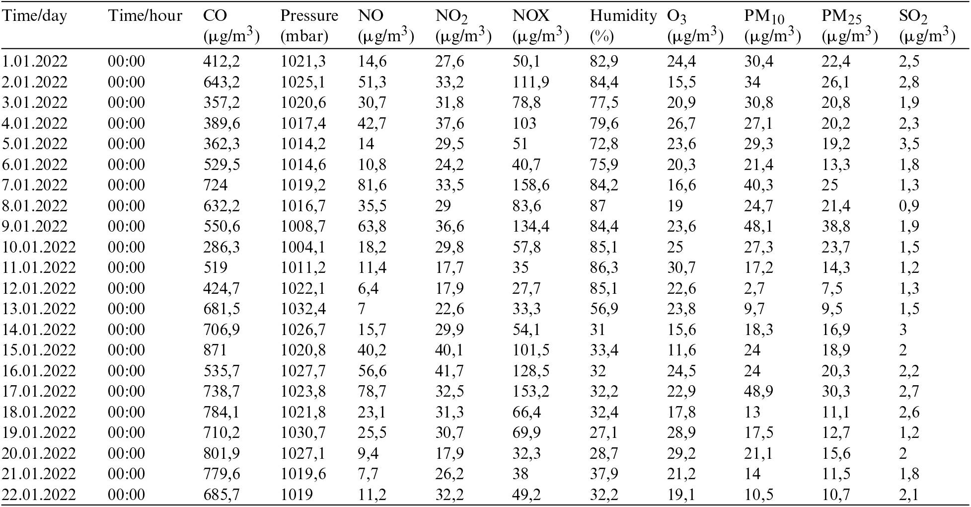
The data used in the study was provided by the Istanbul Air Quality Monitoring Network which included hourly values for a total of 356 days between January 01, 2022, and January 01, 2023. Fig. 1 shows dust-related PM10 and PM25 values, while Fig. 2 shows some values for greenhouse gases. Moreover, Fig. 3 shows rain, temperature, and wind speed values related to weather. A chart representing the solar irradiation value throughout the year can be seen in Fig. 4.

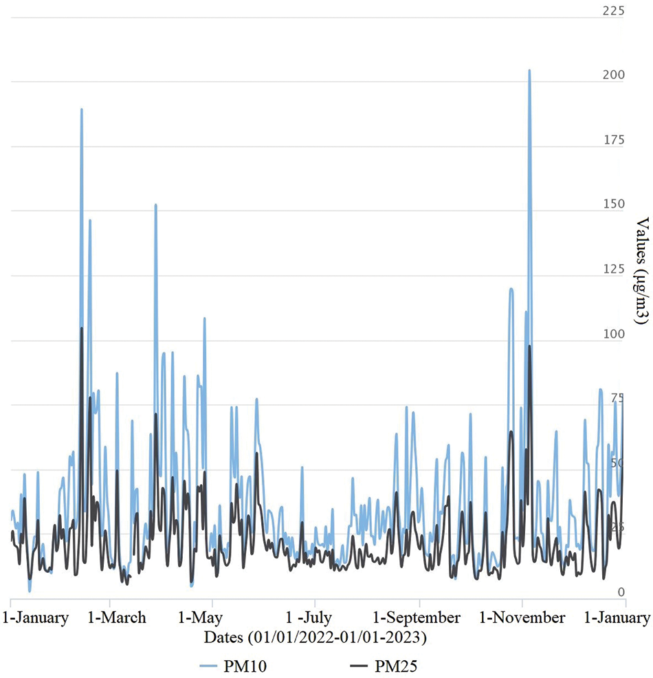
Figure 1: Measurements related to dust (x-axis: time|y-axis: µg/m3)

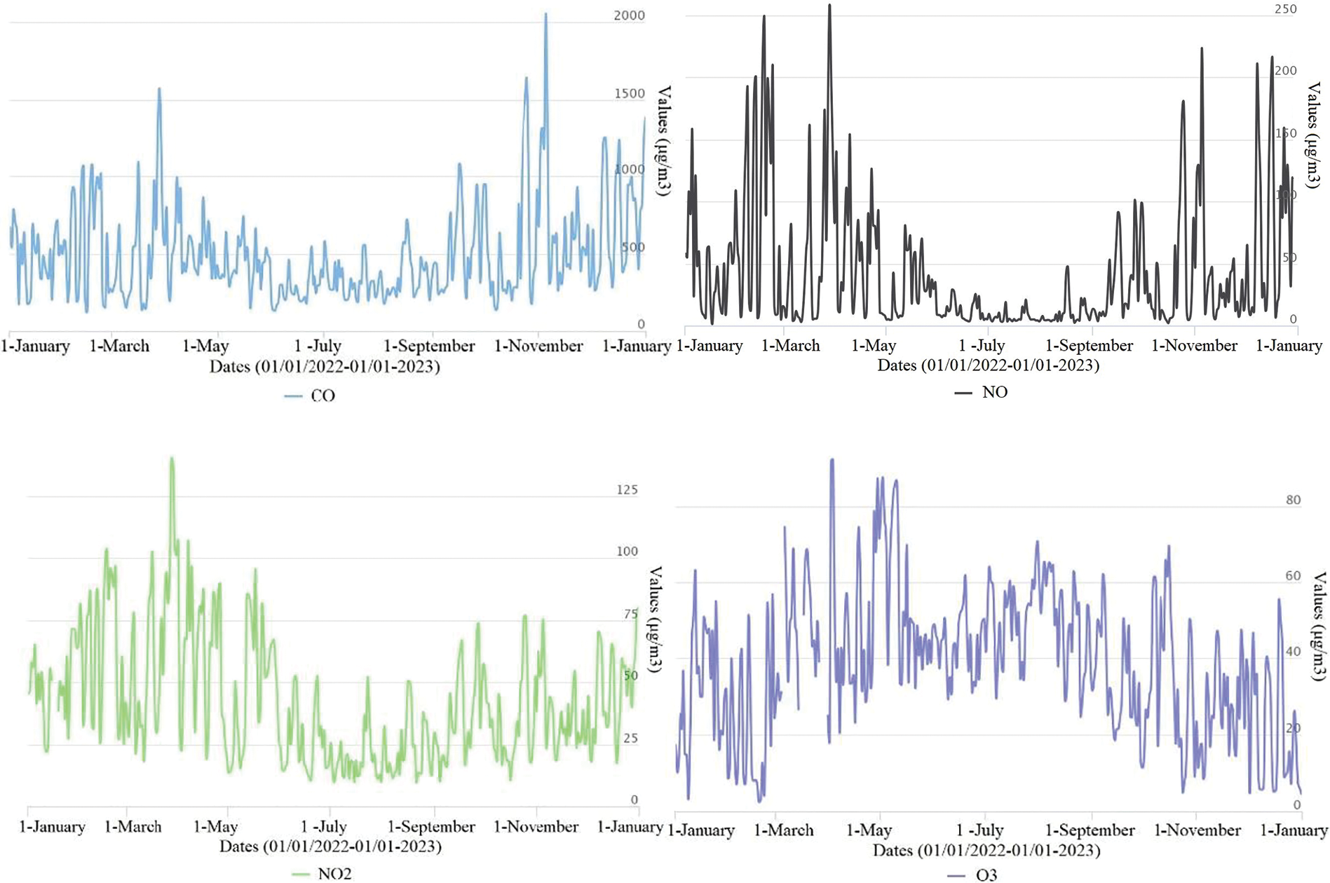
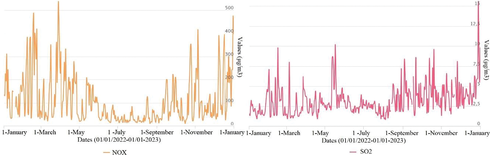
Figure 2: Values related to some greenhouse gases & aerosols (x-axis: time|y-axis: µg/m3)

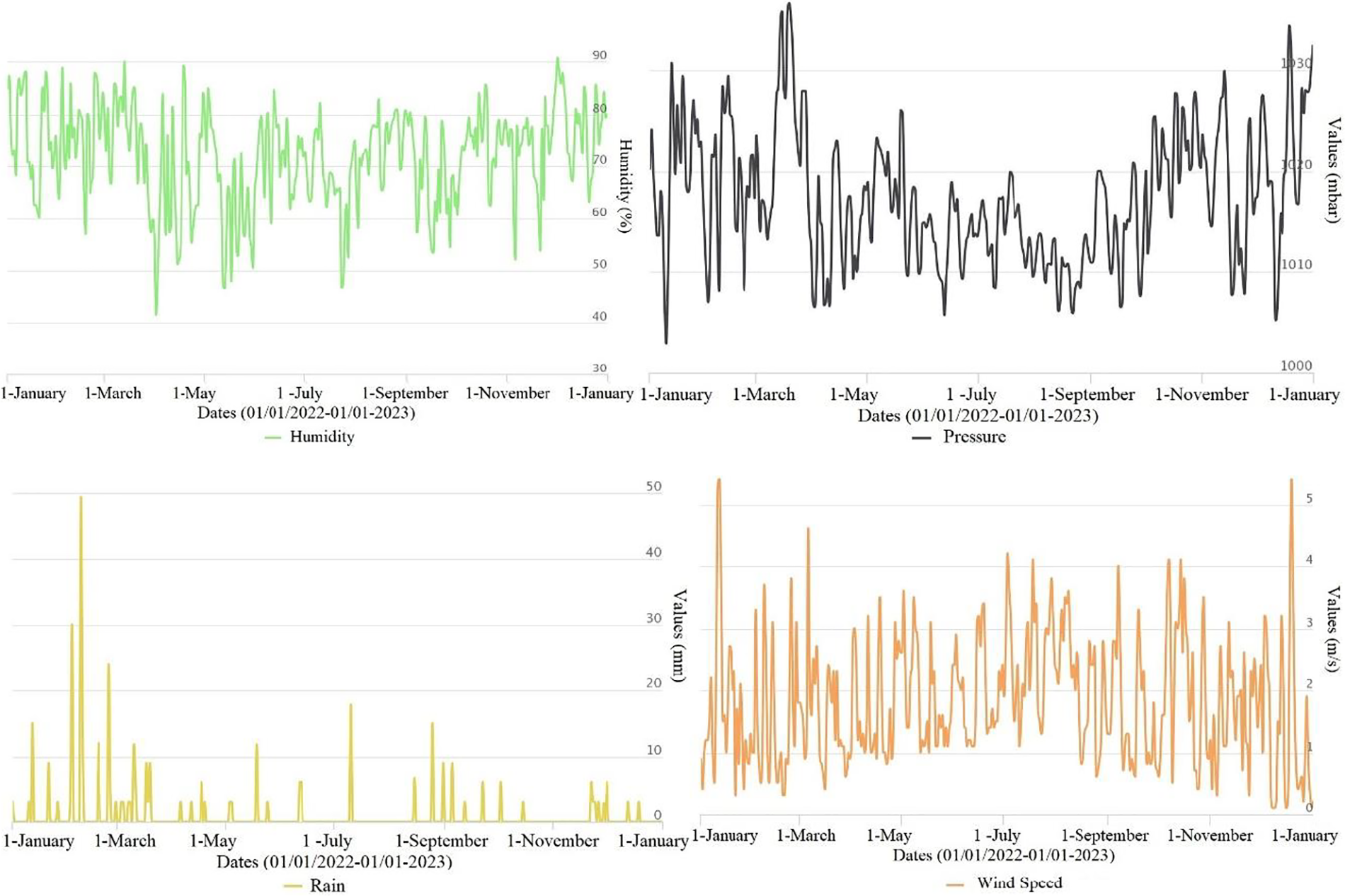
Figure 3: Associated values with weather conditions

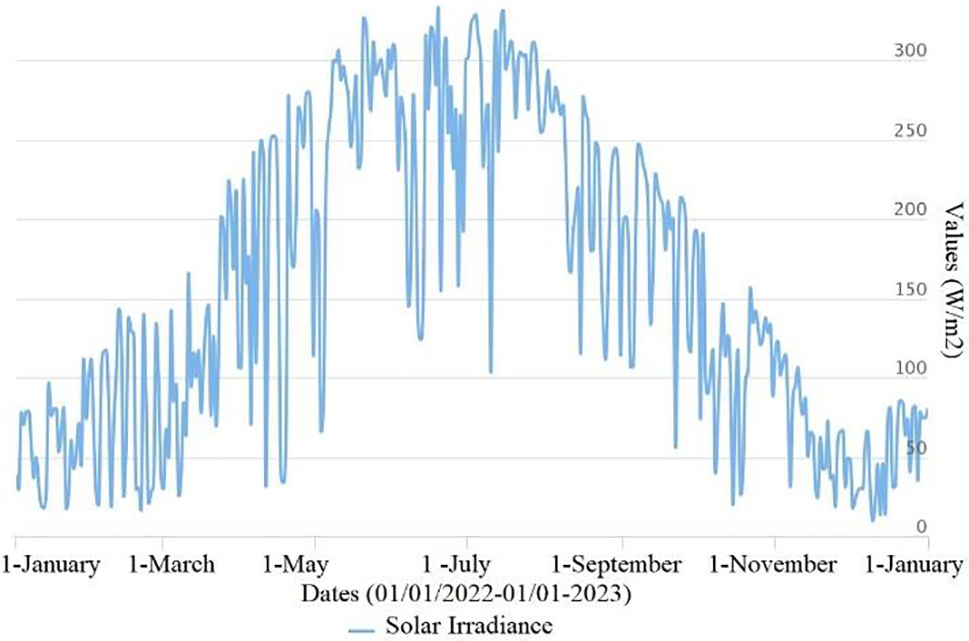
Figure 4: Solar irradiance values (x-axis: time|y-axis: W/m2)

2.2 Convolutional Neural Network (CNN)

Over the years, CNN’s achieved capability to extract features has allowed it to be successfully applied in a wide variety of fields. Therefore, the spatial characteristics of data captured efficiently can reveal a wealth of information about solar radiation. The influence of weather and air pollution on the concentration change of solar irradiance was revealed by extracting the spatial features of solar irradiance (SI). As shown in Fig. 5, the raw data utilized in the paper includes PM10, PM25, CO, NO, NO₂, NOX, O₃, SO₂, humidity (H%), rain (mm), atmospheric pressure (mbar), wind speed (m/s), air temperature (°C) and solar irradiance (W/m2).

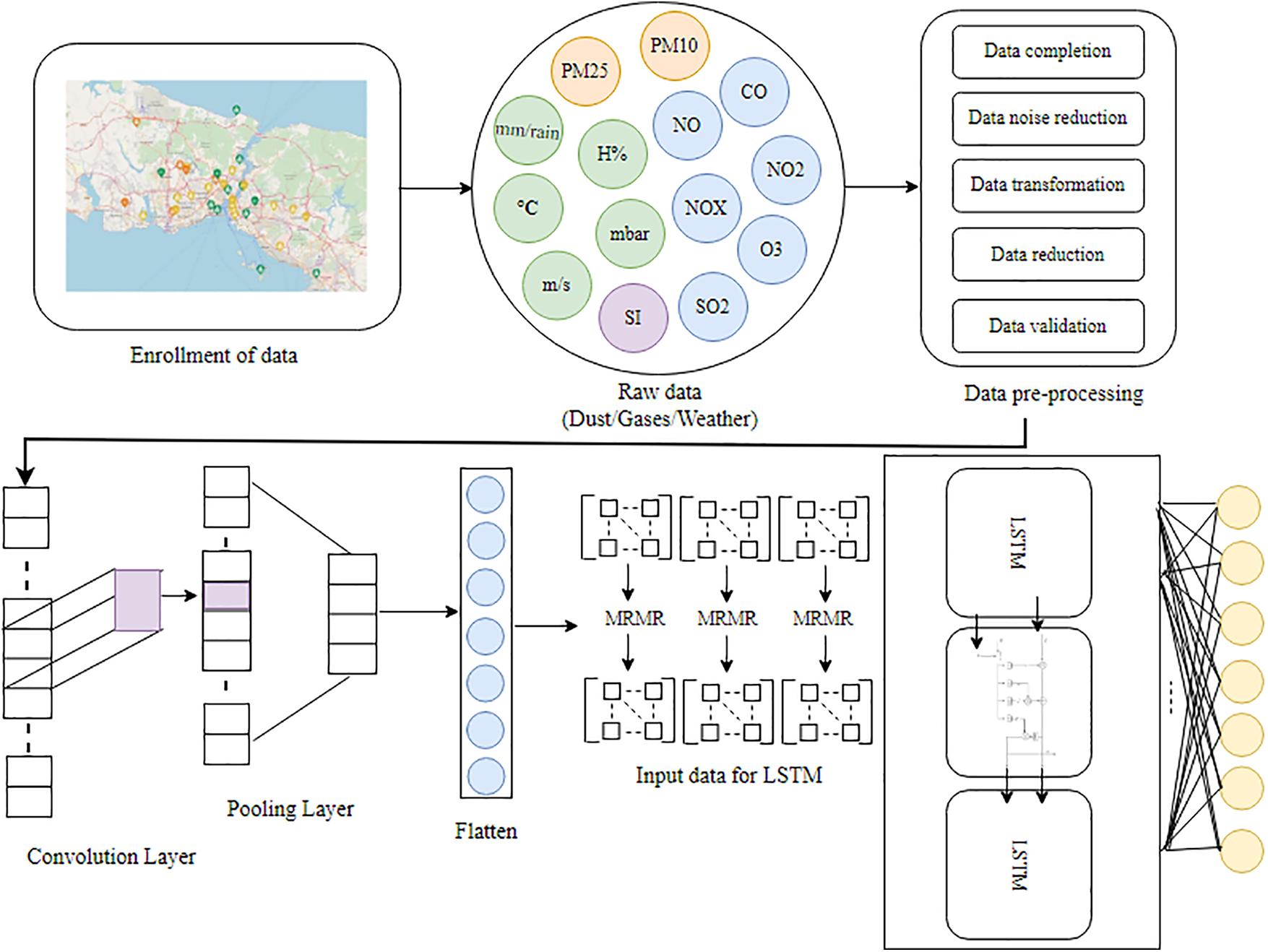
Figure 5: Proposed framework

CNNs differ from traditional neural networks in how they are composed of three layers: convolution, pooling, and full connection layers. CNN’s proposed feature extraction block consists of three layers of convolution in one-dimensional (1D) in the study. The convolution and pooling layers are computed as:

yi=f(wi∗xi+bi)(1)

γ(yi,yi−1)=max(yi,yi−1)(2)

pi=γ(yi,yi−1)+δi(3)

where xi is the input to the convolution layer, representing the pre-processed concentration values of PM10, PM25, CO, NO, NO₂, NOX, O₃, SO₂, humidity (H%), rain (mm), atmospheric pressure (mbar), wind speed (m/s), air temperature (°C) and solar irradiance (W/m2). yi is the feature mapping of the ith output, wi is the weight matrix, * indicates the dot product, bi and δi are bias vectors, f(.) denotes the activation function, γ(.) denotes the sampling function, pi represents the output of the pooling layer after the convolution operation. Convolution layers were separated by MaxPooling and Rectified Linear Unit (ReLU) as seen in Table 1.

A pooling layer is typically included after the convolutional layer to mitigate the limitation of the invariance of the created feature map, whilst the activation function is used to improve the model’s capacity to learn complex structures. The LSTM network structure lies behind this step in the system’s flow.

2.3 Long Short-Term Memory (LSTM)

As opposed to traditional neural networks, which suffer from vanishing gradients, Long Short-Term Memory (LSTM) is a recurrent neural network designed to overcome this problem. It occurs when gradients used to update a network’s weights become very small during backpropagation, making it difficult for the network to learn from long-term dependencies in the data. In addition to capturing both local and temporal variations in solar irradiance, the CNN-LSTM model can also anticipate future conditions by integrating spatial awareness and temporal memory. It combines the extracted features from the CNN with the temporal information learned by the LSTM. Input sequences to the LSTM layer can include the output from the CNN and other relevant time-dependent features. Since LSTM networks are able to remember information for long periods of time, they can capture sequential patterns effectively. The flow of information into and out of each memory cell is controlled by three types of gates: input gates, output gates, and forget gates. During training, the LSTM network learns to selectively store or discard information in the memory cells based on the input data and the current state of the network. The input gate determines which information to store in the memory cells, while the forget gate determines which information to discard. The output gate then determines which information to output from the memory cells to the next layer of the network. The structure diagram of LSTM is seen in Fig. 6.

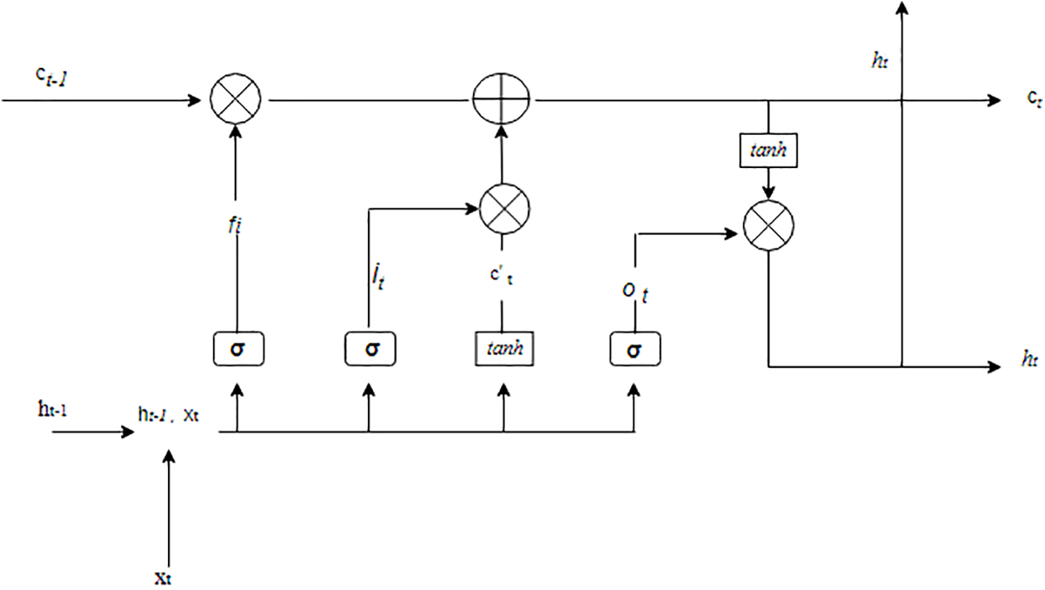
Figure 6: Structure of LSTM

Variables:

xt∈Rd: input vector to the LSTM unit

ft∈(0,1)h: forget gate’s activation vector

it∈(0,1)h: input/update gate’s activation vector

ot∈(0,1)h: output gate’s activation vector

ht∈(−1,1)h: hidden state vector also known as output vector of the LSTM unit

ct′∈(−1,1)h: cell input activation vector

ct∈Rh: cell state vector

W∈Rhxd,U∈Rhxhandb∈Rh: weight matrices and bias vector parameters which need to be learned during training where the superscripts d and h h refer to the number of input features and the number of hidden units, respectively.

An output vector between 0 and 1 is generated by passing the current input and the previous hidden state through a sigmoid function. The hidden state is the output of the LSTM network at each time step. It is a combination of the current memory cell state and the output gate values. As part of the training process, the network parameters are updated according to an optimizing algorithm using backpropagation through time (BPTT), which is a method for computing the gradient of the loss in each time step.

2.4 Maximum Relevance Minimum Redundancy (mRMR)

One of the most important aspects of our approach is that we use the mRMR method for feature selection. A feature selection algorithm called mRMR creates a subset within which related data properties are extracted and unrelated ones are discarded. The algorithm calculates the similarities between each attribute of X and Y by taking into account the mutual information between the two attributes.

I(X,Y)=∑y∈Y∑x∈Xp(x,y)log⁡(p(x,y)p1(x)p2(y))(4)

There are two marginal probability distribution functions, p1(x) and p2(x), and p(x,y) represents the combined probability distribution function.

As a convenient and easy way to express each attribute fi, we will define it as a vector with N observations.

fi=[fi1,fi2,…fiN](5)

It is expressed in the form I(Fi,Fj) where i = 1,2,...,d; j = 1,2,...,d represents the number of attributes in the dataset. The first condition is that S is set of attributes to be selected, |S| is number of elements of a cluster. As a second condition, S must comply with a minimum level of redundancy.

minW,W=1|S|2=∑Fi, Fj∈SI(Fi,Fj)(6)

The maximum relevance condition:

maxV,V=1|S|=∑Fi∈SI(Fi,H)(7)

A similarity result is known as I(Fi,H). Two conditions can be expressed as follows:

max(V−W)(8)

max(V/W)(9)

The attribute that provides a solution for equality (10) and (11) is selected in each subsequent step.

maxFi∈ΩSI(H,Fi)(10)

minFi∈ΩS1|S|∑Fi∈sI(Fi,Fj)(11)

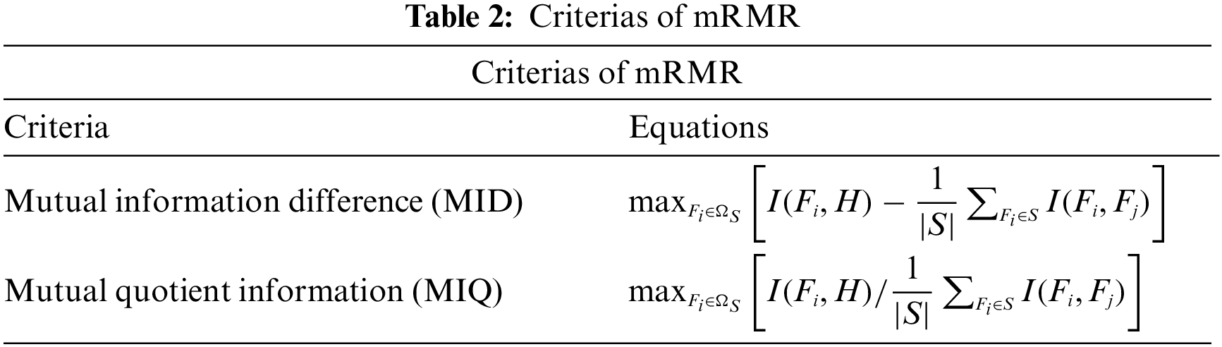
As a result of combining equality (10) and (11) with their respective criteria (8) and (9), the following selection criteria have been generated as seen in Table 2.

3  Results and Discussion

The data of PM10 concentration is collected as a dependent variable and solar irradiance is collected as an independent variable for regression analysis. This data covers a total of 43,791 h of weather analysis results and is collected at a frequency that matches the dynamics of the relationship we are investigating. The scatter plot seen in Fig. 7 visualizes the relationship between PM10 and solar irradiance. The regression formulation utilized in the figure is this:

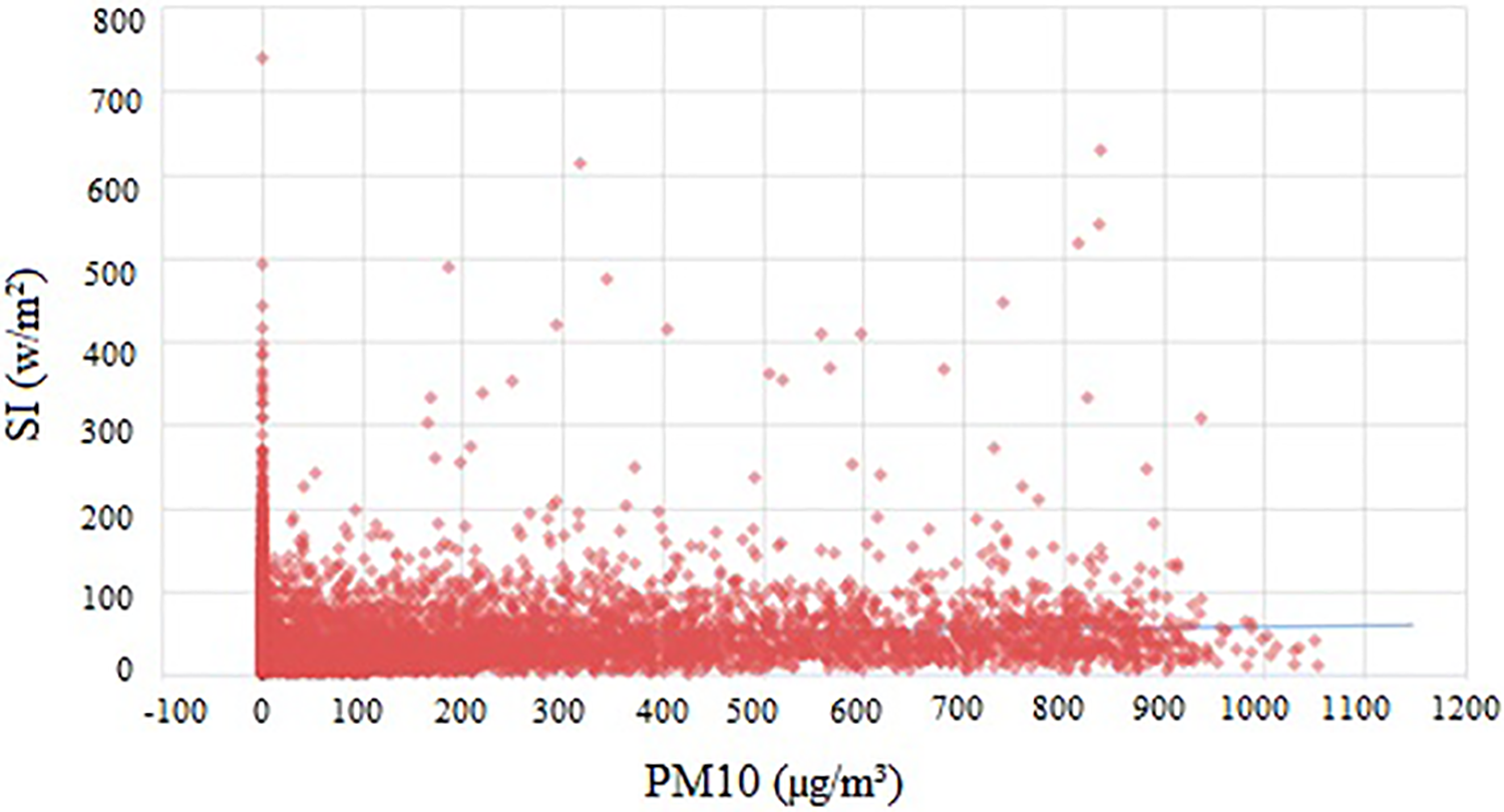
Figure 7: Regression analysis output between solar irradiance and PM10

r=n∑xy−(∑x∑y)n(∑x2)−(∑x)2n(∑y2)−(∑y)2(12)

r = 0.072843 is an output of this regression and presents their power of plain relationship to evaluate the harmony. After examining plain relations then forecasting step is implemented.

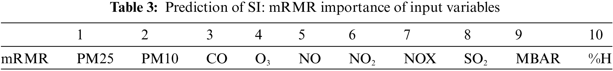
There is also an mRMR analysis performed for each variable to determine how important it is for solar irradiance prediction which is seen in Table 3. PM25 concentration at time t + 1 has the greatest mutual information with solar irradiance at time t. Since mRMR considers irrelevant redundancies as well, other variables must have had a lower redundancy scores. According to the rankings, the next ranks are in the next positions, most likely because they appear to be redundant with SI.

The forecasting process is applied to the data between 01/01/2022 and 01/01/2023 to evaluate the goodness of fit of our model which is seen in Fig. 8. Understanding how much the solar irradiance is expected to change in this context will be revealed by interpreting the results for PM10 concentration. Mean absolute percentage error (MAPE = 6.93) confirms the statistical significance of the relationship, which is important for determining whether or not it is genuine.

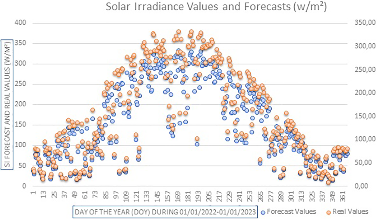
Figure 8: Solar Irradiance values and the forecast results obtained by the suggested model

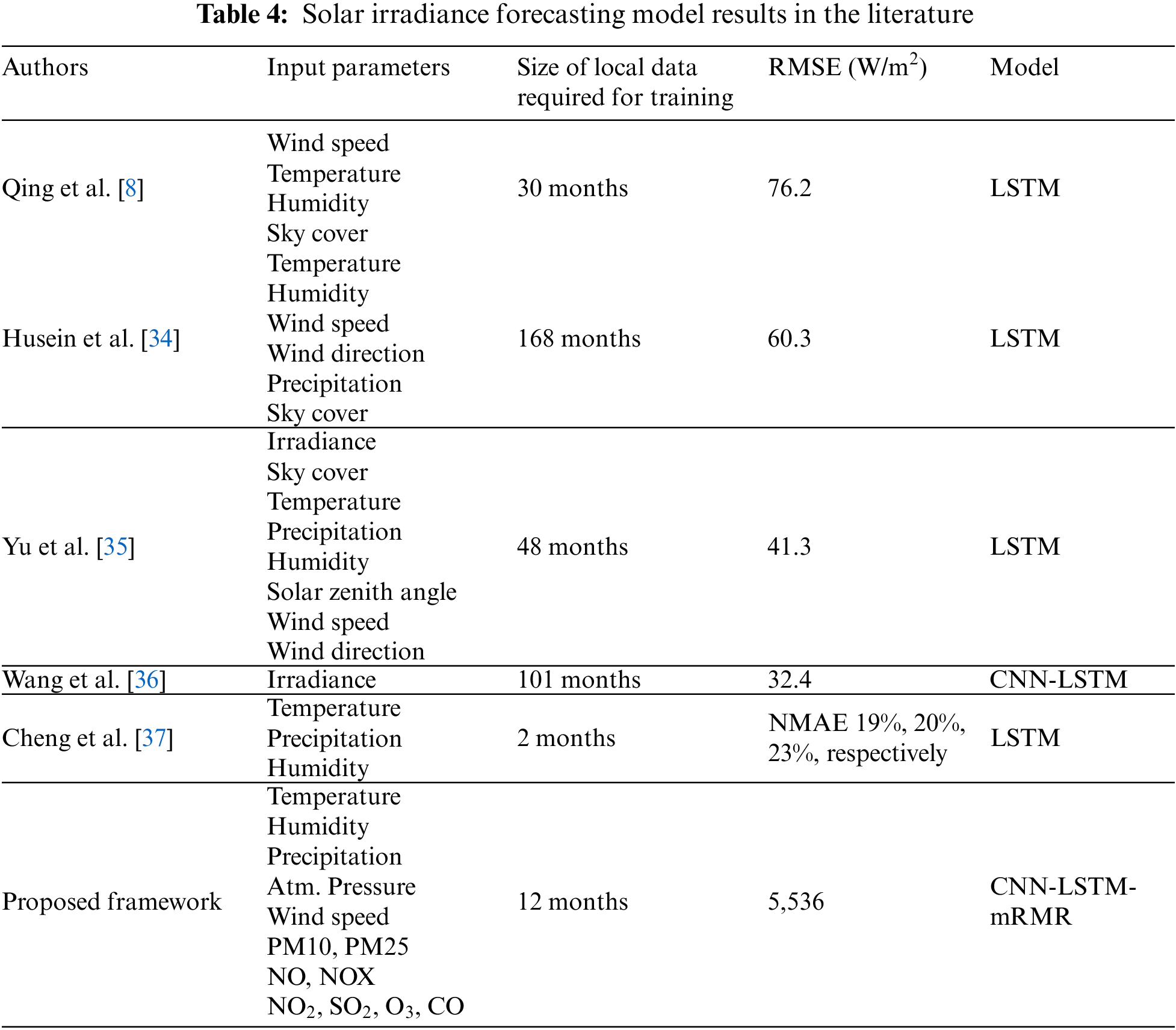
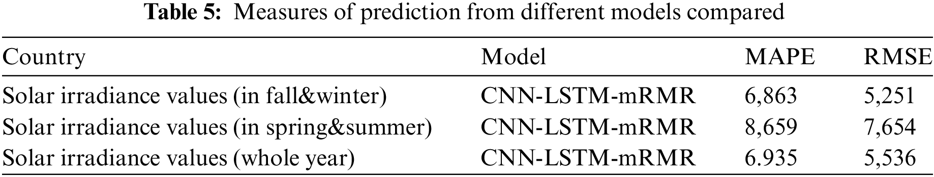
The types of models in the literature are shown in Table 4 along with the corresponding input parameters, forecasting horizon, and time. The results of using the presented model for predicting solar irradiance values can also be seen in Table 5. A total of two error measures are used to evaluate the performance of the proposed models, including root mean square error (RMSE), and mean absolute percentage error (MAPE). Performance scores are derived based on the aforementioned metrics. The error measures RMSE and MAPE values of the Istanbul dataset by CNN-LSTM-mRMR approach are 5,251 and 6,863 in the fall & winter seasons, respectively. The values for the spring & summer seasons are a little bit higher as 7,654 and 8,659, respectively. Whole-year values are 5,536 and 6,935. The approach is robust based on these reliable scores.

4  Conclusions

The present study investigates the effect of air pollutants on solar irradiance using a novel forecasting approach. A thorough analysis of the impact of weather conditions, greenhouse gases, and dust on solar energy systems is the backbone of the search. Solar irradiance could be enhanced to a great extent by improving air quality, as shown by MAPE and RMSE results, 6,935 and 5,536, respectively, and this speeds up the adoption of renewable energy. In other words, air pollution has a strong correlation with reducing effectiveness, particularly in the form of a decrease in the intensity of sunlight, which can have a significant impact on those who invest their capital and wait a short period for a return on investment (ROI). The time of ROI increases, and so does the cost of investing in such energy systems. Furthermore, low effectiveness can discourage government support for renewable energy investments by limiting incentives, like tax credits and rebates, for investors to switch to a more affordable and environmentally friendly mode of green energy.

It is clear from the study that air pollution has a remarkable impact on solar energy systems. A clean environment of decreasing air pollution is prompting the transition to green energy. The nature of the relationship may be complex, and further analysis or additional variables may be needed for a comprehensive understanding. A future study should focus on additional air data, behavioral characteristics of another gas, and using this data to draw meaningful conclusions.

Please visit the link for all data: https://havakalitesi.ibb.gov.tr/STN/VWSTN_Reports/.

Acknowledgement: None.

Funding Statement: The author received no specific funding for this study.

Author Contributions: The author confirms contribution to the paper as follows: Conceptualization, formal analysis, methodology and implementation, analysis and interpretation of results, writing— original draft, review and editing are made by Ramiz Görkem Birdal. The author reviewed the results and approved the final version of the manuscript.

Availability of Data and Materials: Data available on request from the authors.

Conflicts of Interest: The authors declare that they have no conflicts of interest to report regarding the present study.

References

1. R. Heffron et al., “Justice in solar energy development,” Sol. Energy, vol. 218, pp. 68–75, 2021. doi: 10.1016/j.solener.2021.01.072. [Google Scholar] [CrossRef]

2. T. S. Ge et al., “Solar heating and cooling: Present and future development,” Renew. Energy, vol. 126, pp. 1126–1140, 2018. doi: 10.1016/j.renene.2017.06.081. [Google Scholar] [CrossRef]

3. M. A. Gulzar, H. Asghar, J. Hwang, and W. Hassan, “China’s pathway towards solar energy utilization: Transition to a low-carbon economy,” Int. J. Environ Res. Publ. Health., vol. 17, no. 12, pp. 4221, 2020. doi: 10.3390/ijerph17124221. [Google Scholar] [PubMed] [CrossRef]

4. M. Salimi, M. Hosseinpour, and T. N. Borhani, “Analysis of solar energy development strategies for a successful energy transition in the UAE,” Process., vol. 10, no. 7, pp. 1338, 2022. doi: 10.3390/pr10071338. [Google Scholar] [CrossRef]

5. P. Kumari and D. Toshniwal, “Impact of lockdown measures during COVID-19 on air quality–A case study of India,” Int. J. Environ Health. Res., pp. 1–8, 2020. doi: 10.1080/09603123.2020.1778646. [Google Scholar] [PubMed] [CrossRef]

6. W. de Soto, S. A. Klein, and W. A. Beckman, “Improvement and validation of a model for photovoltaic array performance,” Sol. Energy, vol. 80, no. 1, pp. 78–88, 2006. doi: 10.1016/j.solener.2005.06.010. [Google Scholar] [CrossRef]

7. A. Dolara, S. Leva, and G. Manzolini, “Comparison of different physical models for PV power output prediction,” Sol. Energy, vol. 119, pp. 83–99, 2015. doi: 10.1016/j.solener.2015.06.017. [Google Scholar] [CrossRef]

8. X. Qing and Y. Niu, “Hourly day-ahead solar irradiance prediction using weather forecasts by LSTM,” Energy, vol. 148, pp. 461–468, 2018. doi: 10.1016/j.energy.2018.01.177. [Google Scholar] [CrossRef]

9. S. Srivastava and S. Lessmann, “A comparative study of LSTM neural networks in forecasting day-ahead global horizontal irradiance with satellite data,” Sol. Energy, vol. 162, pp. 232–247, 2018. doi: 10.1016/j.solener.2018.01.005. [Google Scholar] [CrossRef]

10. M. Ding, L. Wang, and R. Bi, “An ANN-based approach for forecasting the power output of photovoltaic system,” Procedia Environ. Sci., vol. 11, pp. 1308–1315, 2011. doi: 10.1016/j.proenv.2011.12.196. [Google Scholar] [CrossRef]

11. G. Cervone, L. Clemente-Harding, S. Alessandrini, and L. Delle Monache, “Short-term photovoltaic power forecasting using artificial neural networks and an analog ensemble,” Renew. Energy, vol. 108, no. 1, pp. 274–286, 2017. doi: 10.1016/j.renene.2017.02.052. [Google Scholar] [CrossRef]

12. A. Mellit, S. Sağlam, and S. A. Kalogirou, “Artificial neural network-based model for estimating the produced power of a photovoltaic module,” Renew. Energy, vol. 60, pp. 71–78, 2013. doi: 10.1016/j.renene.2013.04.011. [Google Scholar] [CrossRef]

13. M. Khodayar and J. Wang, “Spatio-temporal graph deep neural network for short-term wind speed forecasting,” IEEE Trans. Sustain. Energy, vol. 10, no. 2, pp. 670–681, 2018. doi: 10.1109/TSTE.2018.2844102. [Google Scholar] [CrossRef]

14. A. Muhammad, J. M. Lee, S. W. Hong, S. J. Lee, and E. H. Lee, “Deep learning application in power system with a case study on solar irradiation forecasting,” in 2019 Int. Conf. Artif. Intell. Inf. Commun. (ICAIIC), 2019, pp. 275–279. [Google Scholar]

15. S. Mishra and P. Palanisamy, “An integrated multi-time-scale modeling for solar irradiance forecasting using deep learning,” 2019. arXiv preprint arXiv:1905, 02616. [Google Scholar]

16. T. P. Chu, J. H. Jhou, and Y. G. Leu, “Image-based solar irradiance forecasting using recurrent neural networks,” in 2020 Int. Conf. Sys. Sci. and Eng.(ICSSE), 2020, pp. 1–4. [Google Scholar]

17. G. Guariso, G. Nunnari, and M. Sangiorgio, “Multi-step solar irradiance forecasting and domain adaptation of deep neural networks,” Energies, vol. 13, no. 15, pp. 3987, 2020. doi: 10.3390/en13153987. [Google Scholar] [CrossRef]

18. A. Mukherjee, A. Ain, and P. Dasgupta, “Solar irradiance prediction from historical trends using deep neural networks,” in 2018 IEEE Int. Conf. on Smart Energy Grid Eng., 2018, pp. 356–361. [Google Scholar]

19. T. A. Farrag and E. E. Elattar, “Optimized deep stacked long short-term memory network for long-term load forecasting,” IEEE Access, vol. 9, pp. 68511–68522, 2021. doi: 10.1109/ACCESS.2021.3077275. [Google Scholar] [CrossRef]

20. M.Ş. Özçoban, M. E. Isenkul, S. Sevgen, S. Acarer, and M. Tüfekci, “Modelling the effects of nanomaterial addition on the permeability of the compacted clay soil using machine learning-based flow resistance analysis,” Applied Sciences, vol. 12, no. 1, pp. 186, 2021. doi: 10.3390/app12010186. [Google Scholar] [CrossRef]

21. D. Chandola, H. Gupta, V. A. Tikkiwal, and M. K. Bohra, “Multi-step ahead forecasting of global solar radiation for arid zones using deep learning,” Procedia Comp. Sci., vol. 167, pp. 626–635, 2020. doi: 10.1016/j.procs.2020.03.329. [Google Scholar] [CrossRef]

22. X. Zhao, H. Wei, H. Wang, T. Zhu, and K. Zhang, “3D-CNN-based feature extraction of ground-based cloud images for direct normal irradiance prediction,” Sol. Energy, vol. 181, pp. 510–518, 2019. doi: 10.1016/j.solener.2019.01.096. [Google Scholar] [CrossRef]

23. F. Wang et al., “Deep learning based irradiance mapping model for solar PV power forecasting using sky image,” in 2019 IEEE Industry App. Society Annual Meeting, 2019, pp. 1–9. [Google Scholar]

24. O. El Alani, M. Abraim, H. Ghennioui, A. Ghennioui, I. Ikenbi and F. E. Dahr, “Short term solar irradiance forecasting using sky images based on a hybrid CNN-MLP model,” Energy. Reports., vol. 7, pp. 888–900, 2021. doi: 10.1016/j.egyr.2021.07.053. [Google Scholar] [CrossRef]

25. Y. LeCun, K. Kavukcuoglu, and C. Farabet, “Convolutional networks and applications in vision,” in Proc. 2010 IEEE Int. Symp. Circuits Syst., 2010, pp. 253–256. [Google Scholar]

26. S. Song, Z. Yang, H. Goh, Q. Huang, and G. Li, “A novel sky image-based solar irradiance nowcasting model with convolutional block attention mechanism,” Ener. Reports., vol. 8, pp. 125–132, 2022. doi: 10.1016/j.egyr.2022.02.166. [Google Scholar] [CrossRef]

27. J. Che, Y. Yang, L. Li, X. Bai, S. Zhang and C. Deng, “Maximum relevance minimum common redundancy feature selection for nonlinear data,” Inform. Sci., vol. 409, pp. 68–86, 2017. doi: 10.1016/j.ins.2017.05.013. [Google Scholar] [CrossRef]

28. P. Verma and H. Om, “MCRMR: Maximum coverage and relevancy with minimal redundancy based multi-document summarization,” Expert. Syst. Appl., vol. 120, pp. 43–56, 2019. doi: 10.1016/j.eswa.2018.11.022. [Google Scholar] [CrossRef]

29. M. Cıbuk, U. Budak, Y. Guo, M. C. Ince, and A. Sengur, “Efficient deep features selections and classification for flower species recognition,” Measurement., vol. 137, pp. 7–13, 2019. doi: 10.1016/j.measurement.2019.01.041. [Google Scholar] [CrossRef]

30. A. R. Webb, “Clustering,” in Statistical Pattern Recognition, Hoboken NJ: John Wiley & Sons, 2003, pp. 361–407. [Google Scholar]

31. Y. Akbulut, A. Sengur, Y. Guo, and F. Smarandache, “NS-k-NN: Neutrosophic set-based k-nearest neighbors classifier,” Symmetry, vol. 9, no. 9, pp. 179, 2017. doi: 10.3390/sym9090179. [Google Scholar] [CrossRef]

32. T. Hastie, R. Tibshirani, J. H. Friedman, and J. H. Friedman, The Elements of Statistical Learning: Data Mining, Inference, and Prediction. vol. 2. New York: Springer, pp. 1–758, 2009. [Google Scholar]

33. J. I. E. Hoffman, “Linear regression,” in J. I. E. Hoffman (Ed.Basic Biostatistics for Medical and Biomedical Practitioners, 2nd ed. Academ. Press, 2019, pp. 445–489. [Google Scholar]

34. M. Husein and I. Y. Chung, “Day-ahead solar irradiance forecasting for microgrids using a long short-term memory recurrent neural network: A deep learning approach,” Energies, vol. 12, no. 10, pp. 1856, 2019. doi: 10.3390/en12101856. [Google Scholar] [CrossRef]

35. Y. Yu, J. Cao, and J. Zhu, “An LSTM short-term solar irradiance forecasting under complicated weather conditions,” IEEE Access, vol. 7, pp. 145651–145666, 2019. doi: 10.1109/ACCESS.2019.2946057. [Google Scholar] [CrossRef]

36. F. Wang, Y. Yu, Z. Zhang, J. Li, Z. Zhen and K. Li, “Wavelet decomposition and convolutional LSTM networks based improved deep learning model for solar irradiance forecasting,” Appl. Sci., vol. 8, no. 8, pp. 1286, 2018. doi: 10.3390/app8081286. [Google Scholar] [CrossRef]

37. H. Y. Cheng, C. C. Yu, and C. L. Lin, “Day-ahead to week-ahead solar irradiance prediction using convolutional long short-term memory networks,” Renew. Energy, vol. 179, pp. 2300–2308, 2021. doi: 10.1016/j.renene.2021.08.038. [Google Scholar] [CrossRef]