Anomaly Detection Algorithm of Power System Based on Graph Structure and Anomaly Attention

1  Introduction

As China’s computer technology and artificial intelligence technology continue to mature, more and more industrial equipment to pursue the realization of industrial intelligence. As the core hub of our production and life, the power system is developing rapidly in the direction of large capacity, ultra-high voltage and long distance, and the requirements for safe and reliable operation of power equipment are becoming more and more strict. Therefore, the research and application of fault diagnosis technology for power equipment is of great practical significance. How to improve the accuracy and speed of the fault diagnosis system, so that the system can quickly and effectively find faults, locate faults, and analyze faults, is an important issue in power grid protection. A number of scholars and industry practitioners are currently working on the detection of anomalies in equipment, which can be defined as the problem of finding instances or models in data that deviate from normal behaviors [1]. Depending on the application area, these ‘deviations’ can also be referred to as anomalies, outliers or singularities. Anomaly detection is used in a wide variety of fields, such as cyber security [2], anomaly detection in industrial systems [3], and network security [4] among others. One of the main reasons why anomaly detection is important is that anomalies often indicate important, critical and hard-to-capture information that is crucial to a company. Sheng [5] used multi-sensors to monitor the three main parameters of temperature, smoke and firelight, and uses multi-sensor fusion technology to solve the contradiction between alarm sensitivity and false alarm rate. Liu et al. [6] analyzed the sound data and vibration data of communication room equipment to determine whether the current health status of communication room equipment is abnormal; and predict the development tendency of the health status of communication room equipment and the time point of reaching the dangerous level. Li [7] used a fuzzy neural network combining neural networks and fuzzy theory to analyze the relationship between the various influencing factors and the equipment status in the power dispatch system, and to accurately describe the operation status of the equipment. The above methods do not work well for the detection of high-dimensional time series data. How to capture complex inter-sensor relationships and detect and interpret anomalies that deviate from these relationships is a challenging problem today? In addition to this, existing anomaly detection methods have several drawbacks, such as incorrect data collection, difficulty in parameter tuning, and the need for annotated datasets for training [8]. Recently, deep learning methods have enabled improved anomaly detection in high-dimensional datasets. Transformers [9] has achieved excellent performance in many tasks in natural language processing and computer vision, and as a result an increasing number of researchers are applying Transformers to anomaly detection. Yin et al. [10] proposed an integrated model of convolutional neural networks (CNN) and recursive autoencoders for anomaly detection and used two-stage sliding windows in data preprocessing to learn data features, with results showing better performance on multiple classification metrics. Li et al. [11] used self-supervised models to construct a high-performance defect detection model that detects unknown anomalous patterns in images in the absence of anomalous data. Xu et al. [12] used the Transformer model and incorporated a very large and very small strategy to amplify, the gap between normal and abnormal data points to improve the correct detection rate of the model. To improve the feature extraction of models for non-linear variables, graphs are widely used to describe real-world objects and their interactions. Graph Neural Networks (GNN) [13–16] as de facto models for analyzing graph structured data, are highly sensitive to the quality of a given graph structure. This paper introduces an algorithm for anomaly detection in power systems based on graph structure and anomaly attention [17–19] which uses an unsupervised deep learning approach to detect anomalies in power equipment, omitting the step of manually annotating the dataset. The anomalous data and states are detected by exploiting correlations between multidimensional time series variables. Its validation results show that multidimensional variables can effectively capture the relationships and correlations between equipment operating states, avoiding the problems of limited prediction accuracy and lack of stability associated with single-dimensional data. Its contributions are summarized below:

•   In this paper, a graph structure is established to represent multidimensional time series as directed graphs, enabling the model to learn the dependencies and correlations between multidimensional time data more effectively;

•   In terms of technology, we propose a power system anomaly detection algorithm based on graph structure and anomaly concern to evaluate the healthy operation status of power plant rooms and to conduct unsupervised research on early faults;

•   Based on the traditional transformer model, the Coding-Decoding Anomaly Detection Model (CD-ADM) model proposed in this paper uses a network structure with multiple encoders in series, which solves the problem that there may be too many data features and the anomaly detection capability of the model decreases.

The remainder of the paper is organized as follows. We describe the methodology in Section 2, which includes the utilization of graph structures, graph convolutional networks, and an abnormal attention mechanism. Section 3 outlines the model’s flow, from data preprocessing to the final output. In Section 4, we present the results of our experiments, including evaluation metrics and performance comparisons. Finally, we provide discussion and conclusions in Sections 5 and 6.

2  Materials and Methods

2.1 Graph Structure

The text graph structure is a more complex data structure than linear tables and tree structures, which can transform data from two-dimensional to multidimensional representation. A node can be connected to any node, and the structure formed by connecting all nodes is called a graph structure. In the graph structure, there may be an association between any two nodes, that is, there are various adjacency relationships between nodes. The graph structure is usually expressed as:

G(V,E)(1)

where G represents a graph, V is the set of all nodes in the graph, and E is the set of edges between nodes.

In a power machine room that needs to detect faults, sensors are used to read data such as main bearing temperature, fan speed, N1 CPU temperature, PCH, power supply voltage, etc., to form a multidimensional time series as the input vector X, (1) Multivariate time series: Multivariate time. The sequence can be expressed as:

X=(x1,x2,…,xN)T∈RN×V(2)

where xi∈RT is a univariate time series of length T, and N is the total number of signals, that is, the number of sensors. y∈Y represents the corresponding label, Y={1,2,…,K} represents normal data with k categories. (2) Abnormality: If the label ya of the sample (xa,ya) does not belong to any predefined class, that is, it is abnormal data. Think of sensors as nodes in the graph structure, and the correlations between sensors as edges between graph structures, as shown in Fig. 1.

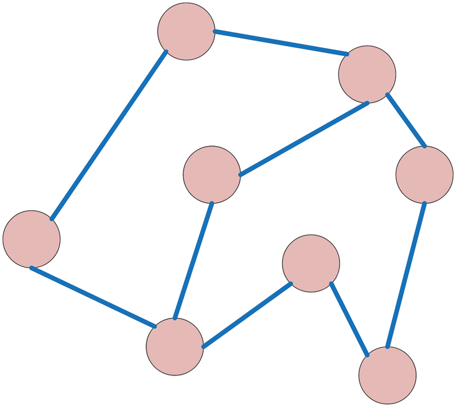
Figure 1: Schematic diagram of graph structure

The definition of a graph is G=(V,E), where V represents the set of nodes and E represents the set of edges.

V={x1,x2,…,xN}(3)

where N represents the number of sensors.

ei∈RN−1,i∈{1,2,…,N}(4)

where ei represents the correlation hypothesis between each sensor and the remaining sensors, and the value range is (0–1).

Since the model does not know the edge information in the graph structure when it is initialized, that is, E is unknown, we randomly initialize E and put it and the adjacency matrix in the model’s graph structure into the graph feature extraction network for training. Here we use the adjacency matrix A to represent the graph structure in a matrix. The sensors corresponding to the multidimensional time series are regarded as nodes in the graph structure, the correlation between sensors is regarded as the edges between nodes in the graph structure, and an adjacency matrix is constructed based on the correlation between nodes in the graph structure.

First, for each sensor node, select relevant nodes to form a candidate node set:

Ci⊆{1,2,…,N}∖{i}(5)

which does not contain i.

In order to express the correlation between sensor node j and candidate node i, the correlation measurement relationship is introduced, expressed by Corji.

Corji=eiTej‖ei‖⋅‖ej‖+log⁡p(xi,xj)p(xi)p(xj),j∈Ci(6)

where the first part is cosine correlation, which is used to measure the correlation between nodes in space, and the latter part is P probability correlation, xi,xj which is used to measure the correlation of nodes in time. Assume that N-dimensional time data obeys Gaussian distribution, where N is the number of sensors, sensor node j and candidate node i are respectively xi,xj, then

p(x)=12πσexp⁡(−(x−μ)22σ2)(7)

p(xi,xj)=12πσexp⁡(−(xixj−μ)2σ2)(8)

where μ,σ represent the mean and variance, respectively. In the formula, Corji represents the correlation between nodes xi,xj,ei is the correlation hypothesis between the node xi and other nodes, the value range is (0–1), p(xi,xj) represents the probability that the node data appears together in the multidimensional l time series in the multidimensional l time series, p(xi) is the probability that node data appears in a multidimensional time series. Ci is the set of related nodes of node. Combining the two dimensions of space and time, the dependence between nodes can be expressed more effectively and the topological structure of the nodes can be refined. The larger the result of Corji, the more similar the two nodes are. The elements of the adjacency matrix Aji are expressed as:

Aji=1{j∈TopK({Corki:k∈Ci})}(9)

Using Eq. (6), first calculate the correlation between sensor i and candidate node j, and then select the first k values, ( N 3 < K < N), where the k value here can be selected according to the complexity of the graph structure expected to be designed by the user, and k the adjacency matrix element corresponding to the value is set to 1, and the rest are 0.

Merge the adjacency matrix A with the additional weight E of the graph structure to obtain the aggregation matrix A^, that is:

A^=G(A,E)=αA+(1−α)E(10)

where α∈(0,1) is the preset graph structure complexity coefficient, which is selected according to the complexity of the actual network.

2.2 Graph Convolutional Network (GCN)

Graph convolutional neural network [20–22], is a type of neural network that convolves the graph structure and is essentially a feature extractor. Since the graph structure is more complex and irregular than the tree structure, it can be regarded as a kind of infinite dimensional data, and it does not have translation invariance during data processing. Therefore, CNN and Recurrent Neural Network (RNN) cannot be used for feature extraction. However, because nodes in the graph structure are easily affected by neighboring nodes, they will also affect other nearby nodes. Under the influence of this interdependence, the nodes will reach a final equilibrium state. Taking advantage of this feature, graph convolutional neural networks can complete feature extraction of graph structures. This article builds a lightweight convolutional neural network to extract features of the graph structure. The parameters of the convolution kernel here are 3 * 3. The input of the network is an aggregation matrix, which is an N-order square matrix, where N represents the number of sensors. That is, the dimensions of multidimensional time series. Due to the lightweight characteristics of the convolutional network, the network is easy to transplant and embed. The graph convolutional neural network shown in Fig. 2, can be used to learn the correlation of adjacent nodes, that is, to build a feature extractor based on the aggregation matrix to learn the information in the graph structure and connect the nodes with surrounding nodes.

Figure 2: Graph convolutional neural network for feature extraction of graph structures

The input aggregation matrix is A^, its dimension is (N * N * T), N is the number of sensors, T is the time series of signals intercepted through the sliding window, the sequence length is T, and the parameters of the convolution kernel are 3 * 3. After adding the pooling layer, the features are compressed through downsampling, the parameters of the fully connected layer are reduced, and the complexity of the model is reduced. Finally, through the fully connected layer, each node of the adjacency matrix is represented as a weighted sum of related nodes. Where, the i of each node, after passing through the convolution pooling-fully connected layer, is comprehensively expressed as:

Gi(t)=WConv(xi(t))+∑j∈N(i)WConv(xj(t))(11)

where Xi(t)∈RN is the input feature of node i, Conv(xi(t)) represents the structure of Xi(t) the convolution pooling layer, N(i)={j|Aji=1} is the set of neighbor nodes connected to node i, W∈Rd×N is the trainable weight matrix, and performs shared linear transformation for each node:

gi(t)=ei⊕Wxi(t)(12)

Zi=exp⁡(gi(t))∑j∈Ci⁡exp⁡(gj(t))(13)

where ⊕ represents the concatenation, therefore, gi(t) connects the sensor correlation hypothesis ei with the corresponding transformed feature Wxi(t), and uses the Sigmoid() function layer for activation. The graph convolutional neural network maps the elements in the input aggregation matrix such that each value belongs to (0, 1) and the sum of all values is 1, i.e., the output is a representation of N nodes, i.e., {z1(t),…,zN(t)}, and the top K are selected from them A connection to the node is established with a large value probability.

Through the convolutional neural network extracted from graph structure features, the model output is the representation of N nodes, that is {z1(t),…,zN(t)}, the loss function is expressed as:

h(t)=‖V1∗Z1+…+Vj∗Zj‖2−‖V1∗Cor1+…+Vj∗Corj‖2(14)

2.3 Abnormal Attention Mechanism

Literature [12] improved the structure of the transformer and proposed two methods for calculating correlation, namely a priori correlation and a sequence correlation. The prior correlation mainly represents the correlation between each time point and adjacent time points, while the sequence correlation The focus is on the correlation between each time point and the entire sequence. In view of this, the network structure diagram used in the proposed model is shown in Fig. 3. Coding-Decoding Anomaly Detection Model (CD-ADM). That is, the multidimensional time series perceived by the power system is intercepted through a sliding window, and a time series of length T is intercepted. An encoder based on the anomaly attention mechanism is used for feature extraction, and then the decoder based on the multi-head attention mechanism is used for prediction.

Figure 3: Abnormal attention mechanism structural mode

The reconstruction error of its output is:

Zl=Layer−Norm(Muti−attention(Xl−1)+Xl−1)(15)

Xl=Layer−Norm(feed−forward(Zl)+Zl)(16)

where Xl∈RN∗d,l∈{1,…,L} represents the output of the L-th layer and dmodel channel. The initial input X0=Embedding(X) represents the original sequence of the embedding. Zl∈RN×dmodel represents the hidden representation of layer L. The encoder has an unusual attention to two branch structures internally. For the prior correlation, a learnable Gaussian kernel is used to calculate the prior correlation relative to the temporal distance. Since the Gaussian kernel function has only one peak, and the closer the distance to the center point, the closer the similarity is to 1, and vice versa. Taking advantage of this feature, the attention mechanism that introduces the Gaussian kernel function will pay more attention to the features of nearby nodes. Here, a learnable parameter is embedded into the Gaussian kernel function so that the prior correlation adapts to various time series patterns, such as abnormal segments of different lengths. The sequence correlation branch learns correlations from the original sequence and can adaptively find the most effective correlations. The abnormal time series attention model parameters of layer L are: The initial value of Q, K, V is:

Q,K,V,r=Xl−1WQl,Xl−1Wkl,Xl−1Wvl,Xl−1Wrl(17)

where Q,K,V∈RN×dmodel,r∈RN×1 represent the query, keyword, self-attention value and learning amount respectively, WQl,WKl,WVl∈Rd×d,Wrl∈Rd×1 and represent the parameter matrices of Q, K, V, r in the L-th layer, respectively. Serial correlation S is calculated as follows:

Sl=Softmax(QiKiTd)(18)

Due to the rarity of equipment anomalies in power equipment rooms and the dominance of the normal mode, it is difficult to establish a strong correlation between anomalies and the entire sequence. Anomalous correlations should be clustered at adjacent time points, which are more likely to contain similar anomalous patterns due to continuity. This adjacent correlation bias is called a priori correlation. The present invention calculates it and records it as P, and uses the learnable Gaussian kernel r to calculate it. The calculation method is as follows:

Pl=Rescale([12πri2exp⁡(−|j−i|22ri2)]i,j∈{1,…,N})(19)

where r∈RN×1a2+b2, N is the length of the time series involved in the calculation, i, j correspond to different time points, that is, the association weight from the i-th time point to the j-th time point is calculated by the Gaussian kernel:

G(|j−i|;ri)=12πri2exp⁡(−|j−i|22ri2)(20)

Rescale(.) represents the division by row sum operation, which is used to transform the associated weight into a discrete distribution. The model structure of the decoder is shown in Fig. 4 below.

Figure 4: The model structure of the decoder

The reconstruction error is:

Z^L=SLV(21)

As an unsupervised task, we employ a reconstruction loss to optimize our model. The reconstruction loss will guide the series of correlations to find the most informative correlation. To further amplify the differences between normal and abnormal time points, we also use additive losses to amplify the correlation differences. The loss function is:

L=mine,λ,w‖h(t)−h^(t)‖2+λ‖Z^L−X‖2(22)

where e is the additional weight of each node, w is the parameter of the neural network, h(t) is the output obtained after the adjacency matrix of the graph structure passes through the graph neural network, ‖Z^L−X‖2 indicating the sequence obtained by the anomaly detection module based on the self-attention mechanism reconstruction loss. We calculated an anomaly score for each time series on the sensor. Compare the model prediction results with the observed time series, and calculate the error value of sensor i at time t:

Erri(t)=|hi(t)−h^i(t)|+‖Zit−xi(t)‖2(23)

In the formula, Erri(t) represents the error value of the sensor i at the time t, hi(t) represents the weighted set of the node i at the time t connected by other nodes through the edges, hi(t)=x1e1,i+x2e2,i+…+xjej,i, ej,i represents the value of the edge between nodes xi,xj,h^i(t) represents the result of hi(t) after passing through the graph convolutional neural net h^i(t)=x1e^1,i+x2e^2,i+…+xje^j,i, e^j,i, represents the value of the edge between nodes after processing by the graph convolutional neural network, Zit represents the value of the i-th sensor at time in the anomaly detection result, xi(t) represents the observation value of the i-th sensor at time t; Since different sensors may have very different characteristics, their bias values may also have very different scales. To prevent any one sensor from biasing more than the others, we normalize the error values for each sensor:

ai(t)=Erri(t)−μ^iσ^i(24)

where μ^i,σ^i, represent the mean and variance of Erri(t) within the time interval, respectively. To calculate the overall anomaly at time point t, we aggregate the sensors using the max function:

A(t)=maxiai(t)(25)

Set the threshold to the maximum value of the validation set data, that is, exceed the maximum anomaly score of the validation data set. If A(t), exceeds a fixed threshold, the time is marked as an anomaly. We use the data of the previous few days at the current moment for training modeling, and then use the data of the current day as the test set to obtain the anomaly score. This improvement also achieves the ability to detect device anomalies in real time.

3  Equations and Mathematical Expressions

In the experiment, the operating health status of the power computer room is displayed in the form of data, which is used as an evaluation indicator for computer room maintenance. Through a reasonable diagnosis mechanism and status operation monitoring mechanism, the probability of failure in the power machine room will be effectively reduced. The proposed model constructs the following six parts for the abnormal diagnosis process, as shown below: 1. Perceive the signal; 2. Perform preprocessing operations on multidimensional l time series signals and convert them into graph structures; 3. Input the adjacency matrix obtained from the graph structure into the graph neural network, and the model output is a weighted set result between multidimensional time series variables; 4. Pass the original signal through a sliding window of length T and input it into the encoder based on the self-attention mechanism. Multiple encoders are connected in series, and then input into the decoder containing the multi-head attention module, and then the model output is the reconstruction error; 5. Establish a threshold and define anomaly scores exceeding the threshold as anomaly sequences; 6. After an abnormality occurs, start the early warning mode. The abnormal diagnosis flow chart construction is shown in Fig. 5.

Figure 5: Anomaly detection flow chart

4  Results

First, the abnormal model training of the power computer room data set and the verification result analysis are performed. Figs. 6 and 7 below respectively show the verification results of the (long short-term memory) LSTM model and the CD-ADM model on the power computer room test set. The blue solid line represents the real data, the orange dotted line represents the predicted data, and the residual value of the two. It is the green curve.

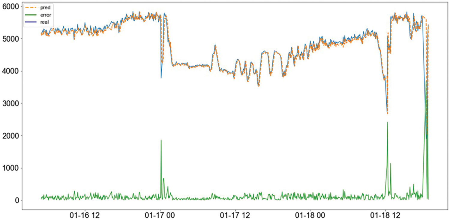
Figure 6: LSTM model test results chart

Figure 7: CD-ADM model test results char

In Figs. 6 and 7, the LSTM model test results show smaller fitting errors, while CD-ADM shows a more obvious residual amount. It is impossible to judge the pros and cons of the two methods just from the above picture. Next, real anomaly points are added, and the prediction error (green curve) is used as the evaluation criterion to determine equipment anomalies. The anomaly detection results in Fig. 8, below are obtained:

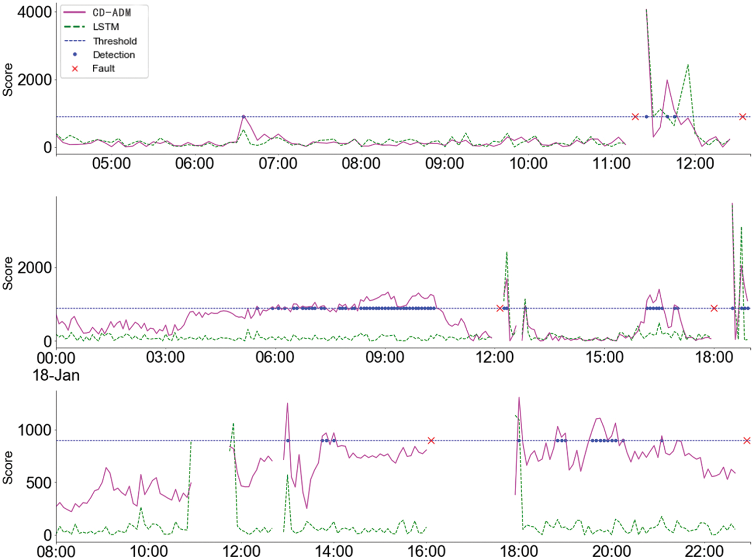
Figure 8: Comparison chart of anomaly detection between LSTM model and CD-ADM model

The pink curve in Fig. 8, above is the anomaly score curve of the CD-ADM model, the green is the anomaly score curve of the LSTM model, and the blue dotted line is the artificially set anomaly judgment threshold. If it is higher than the blue dotted line, it is considered an anomaly. The real points are abnormal alarms detected by the model, and the red crosses are the actual fault occurrence points of the data. The above figure shows that the CD-ADM model can fully learn the characteristics that the device health status should display, and it will also show a gradual upward trend when it is closer to the abnormal point. This is what this experiment hopes the model can learn. Important information. In the first section of the curve, the CD-ADM model and the LSTM model show similar characteristics; in the second section, the former shows a gradually increasing trend than the latter and generates multiple times before the first shutdown for maintenance, warning information, and also showed similar characteristics before the second shutdown; in the third paragraph, it can be seen that the improved model clearly shows an increasing trend, but the trend cannot be seen in the unimproved model. The upward trend shown in the CD-ADM model provides valuable information about the operational health of the equipment, because failures caused by this slow wear are often progressive and avoidable. Figs. 9 and 10 show the fitting performance of the CD-ADM model and LSTM model on normal datasets in power rooms. Comparing the prediction error curves, except for some differences in the time period when the real curve fluctuates, the overall prediction modeling accuracy and fitting effect are maintained very well.

Figure 9: The fitting of CD-ADM on normal data sets in power rooms

Figure 10: The fitting of LSTM on normal data sets in power rooms

5  Discussion

In this study, we proposed a novel approach for abnormal warning detection in power equipment rooms based on graph convolutional attention mechanism. Our results demonstrate that the use of graph convolutional networks with attention mechanism yields promising performance in identifying abnormal patterns within the power equipment rooms. The model showed high accuracy in detecting various anomalies such as temperature fluctuations, humidity deviations, and equipment malfunctions. One of the key strengths of our approach lies in its ability to capture complex relationships and dependencies among different sensors and equipment within the power equipment rooms. By leveraging the graph convolutional attention mechanism, the model can effectively learn and adapt to the dynamic interactions among the various data points, leading to improved abnormal detection capability. However, it is important to acknowledge the limitations of our study. One potential limitation is the dependency on the quality and quantity of the training data. Collecting sufficient and diverse datasets to represent all possible abnormal scenarios remains a challenge. Additionally, the computational complexity associated with graph convolutional networks may hinder real-time deployment in some practical settings.

In future work, it would be beneficial to explore methods for enhancing the robustness of the model against noisy or incomplete data. Furthermore, investigating techniques to optimize the computational efficiency of the graph convolutional attention mechanism would facilitate its implementation in real-time abnormal warning systems. Additionally, the integration of multi-modal data sources and the incorporation of domain knowledge could further improve the model’s performance in capturing complex abnormal patterns.

6  Conclusions

This article uses the encoding-decoding anomaly detection model (CD-ADM) to reproduce the process of abnormal warning in the computer room. This paper proposes the application of deep learning to intelligent detection methods of power equipment room equipment faults, and the use of unsupervised deep learning methods to reduce the labeling of data sets, which greatly saves labor costs and thus improves traditional detection methods. This paper proposes a graph structure to establish correlations between multidimensional data. Traditional anomaly detection methods do not know which sensors are related to each other, so it is difficult to build sensor data with many potential correlations. In addition, traditional graph neural networks use the same model to establish the graph structure for each node, which limits the flexibility of the model. Therefore, we improve the graph-structured feature learning network, add additional weights to each edge, and select the k value for training according to the complexity of the model. Therefore, we can accurately understand the interdependencies between sensors. That is, the multidimensional time series is represented by a graph structure, and the aggregation matrix obtained by the graph structure is input to the feature learning network of the graph structure. Taking advantage of the lightweight characteristics of the network, it is easy to transplant and embed the network, realize nonlinear transformation, enhance the expression ability of the model, and perform end-to-end learning of node feature information and structural information. Finally, this method can effectively learn the correlation between multidimensional time variables, establish the topology of time series, and convert from two-dimensional space to multidimensional space. In addition, based on the self-attention mechanism, the single-branch self-attention module is changed to a dual-branch anomaly attention detection module to improve the model’s ability to distinguish between normal data and abnormal data. In the prediction time series module, in order to avoid the “over-fitting” phenomenon, the gradient disappears and the prediction results are often volatile, which makes the prediction performance of the model unstable. The proposed model can effectively solve the above problems by connecting multiple encoders in series.

Acknowledgement: Thanks to Prof. Dr. Jiande Zhang from Nanjing Institute of Technology for his comments. The authors thanks to all individuals who contributed to the planning, implementation, editing, and reporting of this work but are not listed as authors. Their invaluable support played a significant role in the success of this research.

Funding Statement: This paper was funded by the Science and Technology Project of China Southern Power Grid Company, Ltd. (031200KK52200003), the National Natural Science Foundation of China (Nos. 62371253, 52278119).

Author Contributions: Conceptualization, Yifan Gao; Data curation, Xianchao Chen; Formal analysis, Yifan Gao; Investigation, Zhanchen Chen; Methodology, Yifan Gao, Jieming Zhang and Xianchao Chen; Software, Yifan Gao; Supervision, Xianchao Chen; Validation, Zhanchen Chen; Writing–original draft, Jieming Zhang; Writing–review editing, Zhanchen Chen. All authors reviewed the results and approved the final version of the manuscript.

Availability of Data and Materials: Due to the nature of this research, participants of this study did not agree for their data to be shared publicly, so supporting data is not available. We provide the author’s contact information so that readers in need can get in touch with us and learn more about relevant information.

Conflicts of Interest: The authors declare that they have no conflicts of interest to report regarding the present study.

References

1. X. Xia et al., “GAN-based anomaly detection: A review,” Neurocomputing, vol. 493, pp. 497–535, 2022. doi: 10.1016/j.neucom.2021.12.093. [Google Scholar] [CrossRef]

2. L. Rettig et al., “Online anomaly detection over big data streams,” in Applied Data Science. Cham: Springer, 2019, pp. 289–312. [Google Scholar]

3. X. Zhou, Y. Hu, W. Liang, J. Ma, and Q. Jin, “Variational LSTM enhanced anomaly detection for industrial big data,” IEEE Trans. Industr. Inform., vol. 17, no. 5, pp. 3469–3477, 2021. doi: 10.1109/TII.2020.3022432. [Google Scholar] [CrossRef]

4. R. Ahmad, R. Wazirali, and T. Abu-Ain, “Machine learning for wireless sensor networks security: An overview of challenges and issues,” Sensors, vol. 22, no. 13, pp. 4730, Jun. 2022. doi: 10.3390/s22134730 [Google Scholar] [PubMed] [CrossRef]

5. M. A. Sheng, “Research and design of remote inspection and monitoring system for communication equipment room,” Ph.D. dissertation, Chongqing Univ., China, 2002. [Google Scholar]

6. W. F. Liu, J. P. Yang, H. Zhang, and X. P. Chen, “A method for detecting and analyzing the health status of communication equipment room,” 2018. CN201810293767.6. [Google Scholar]

7. P. Li, “Research and application of the health state assessment method of power dispatch automation equipment,” M.S. thesis, Univ. of Chinese Academy of Sciences, China, 2019. [Google Scholar]

8. T. S. Buda, B. Caglayan, and H. Assem, “Deepad: A generic framework based on deep learning for time series anomaly detection,” in Pacific-Asia Conf. Knowl. Discovery Data Min., Cham, Springer International Publishing, Jun. 2018, pp. 577–588. doi: 10.1007/978-3-319-93034-3_46. [Google Scholar] [CrossRef]

9. A. Vaswani et al., “Attention is all you need,” in NIPS’17, Adv. Neural Inf. Process. Systems, Long Beach California, USA, vol. 30, Dec. 4–9, 2017. [Google Scholar]

10. C. Yin, S. Zhang, J. Wang, and N. N. Xiong, “Anomaly detection based on convolutional recurrent autoencoder for IoT time series,” IEEE Trans. Syst. Man Cybern.: Syst., vol. 52, no. 1, pp. 112–122, Jan. 2022. doi: 10.1109/TSMC.2020.2968516. [Google Scholar] [CrossRef]

11. C. L. Li, K. Sohn, J. Yoon, and T. Pfister, “CutPaste: Self-supervised learning for anomaly detection and localization,” in Proc. IEEE/CVF Conf. Comput. Vis. Pattern Recognit. (CVPR), Jun. 19–25, 2021, pp. 9664–9674. [Google Scholar]

12. J. Xu, H. Wu, J. Wang, and M. S. Long, “Anomaly transformer: Time series anomaly detection with association discrepancy,” ICLR, Apr. 25–29, 2022. 10.48550/arXiv.2110.02642 [Google Scholar] [CrossRef]

13. Y. Zhu et al., “A survey on graph structure learning: Progress and opportunities,” IJCAI, Jul. 23–29, 2022. 10.48550/arXiv.2103.03036 [Google Scholar] [CrossRef]

14. A. Chaudhary, H. Mittal, and A. Arora, “Anomaly detection using graph neural networks,” in 2019 Int. Conf. Mach. Learning, Big Data, Cloud and Parallel Comput. (COMITCon), Faridabad, India, 2019, pp. 346–350. doi: 10.1109/COMITCon.2019.8862186. [Google Scholar] [CrossRef]

15. O. Atkinson, A. Bhardwaj, C. Englert, V. S. Ngairangbam, and M. Spannowsky, “Anomaly detection with convolutional graph neural networks,” J. High Energy Phys., vol. 2021, no. 8, pp. 1–19, 2021. doi: 10.1007/JHEP08(2021)080. [Google Scholar] [CrossRef]

16. A. Deng and B. Hoi, “Graph neural network-based anomaly detection in multivariate time series,” in AAAI-21, Vancouver, Canada, vol. 35, May 2021, pp. 4027–4035. doi: 10.1609/aaai.v35i5.16523. [Google Scholar] [CrossRef]

17. C. Ding, S. Sun, and J. Zhao, “MST-GAT: A multimodal spatial-temporal graph attention network for time series anomaly detection,” Inf. Fusion., vol. 89, pp. 527–536, Aug. 2022. doi: 10.1016/j.inffus.2022.08.011. [Google Scholar] [CrossRef]

18. L. Zhou, Q. Zeng, and B. Li, “Hybrid anomaly detection via multihead dynamic graph attention networks for multivariate time series,” IEEE Access, vol. 10, pp. 40967–40978, Apr. 2022. doi: 10.1109/ACCESS.2022.3167640. [Google Scholar] [CrossRef]

19. Y. Yu, Z. Zha, B. Jin, G. Wu, and C. X. Dong, “Graph-based anomaly detection via attention mechanism,” in ICIC 2022: Intelligent Computing Theories and Application, Xi’an, China, Aug. 7–11, 2022. pp. 401–411. [Google Scholar]

20. Y. Djenouri, A. Belhadi, G. Srivastava, J. Chun, and W. Lin, “Hybrid graph convolution neural network and branch-and-bound optimization for traffic flow forecasting,” Future Gener. Comput. Syst., vol. 139, no. 9, pp. 100–108, Oct. 2022. doi: 10.1016/j.future.2022.09.018. [Google Scholar] [CrossRef]

21. A. Ali, Y. Zhu, and M. Zakarya, “Exploiting dynamic spatio-temporal graph convolutional neural networks for citywide traffic flows prediction,” Neural Netw., vol. 145, no. 2, pp. 233–247, Nov. 2021. doi: 10.1016/j.neunet.2021.10.021 [Google Scholar] [PubMed] [CrossRef]

22. M. Ravinder et al., “Enhanced brain tumor classification using graph convolutional neural network architecture,” Sci. Rep., vol. 13, no. 1, pp. 14938, Sep. 2023. doi: 10.1038/s41598-023-41407-8 [Google Scholar] [PubMed] [CrossRef]