A Hybrid Deep Learning Method for Forecasting Reservoir Water Level from Sentinel-2 Satellite Images

1  Introduction

The water level in reservoirs is necessary to evaluate water resources for different purposes such as irrigation, agriculture, early flood warning, and hydroelectricity [1]. Forecasting water level is important for hydrological studies, significantly affecting water resource management, flood forecasting, and environmental protection. Traditional methods used for forecasting the water level often rely on statistical models. This approach is useful to solve the problem but it still has some limitations in capturing complex and non-linear relationships inherent in water processes, leading literature to low accuracy [2,3]. Recent advances in machine learning have led to the development of various models for hydrological and environmental studies [4,5]. For the forecast of the reservoir water level, many types of traditional and classic models have been evaluated, such as Artificial Neural Network (ANN) [6–8], Adaptive Neuro Fuzzy Inference System (ANFIS) [9–11], and Extreme Learning Machines (ELM) [12–14]. For these models, hydrological data of the reservoir is required.

In recent years, satellite imagery has become a valuable resource in various fields. For instance, Shahab Ul Islam et al. [15] employed remote sensing imagery to assess changes in the spatial distribution and scale of infrastructure in Peshawar District, Pakistan. Similarly, Song et al. [16] used remote sensing imagery for maritime vessels. Another application of remote sensing imagery is in hydrology, where satellite imagery has been widely used. In the studies [17,18], water level forecasting was conducted by providing detailed and continuous spatial data, enabling researchers and experts to monitor water level fluctuations over large areas. Besides, leveraging remote sensing capabilities, satellite imagery can be used to gather water level information in difficult-to-access regions where direct measurements are unfeasible, including flood-prone areas, remote rivers, and large reservoirs [19]. Moreover, satellite imagery offers frequent temporal updates, allowing for timely detection of minor and sudden changes in water levels, thereby enhancing the accuracy and reliability of proposed models [20]. The advancement of remote sensing technology and modern data analysis methods has created new opportunities for extracting data from satellite imagery, improving the effectiveness of research outcomes and water resource management.

Several advanced satellite image segmentation models have been extensively developed. In addition to traditional models such as multiview subspace clustering [21], deep learning models for image segmentation include UNet, Mask R-CNN, SegNet, and YOLO. UNet [22,23] was designed for biomedical segmentation and has demonstrated effectiveness in satellite image processing. Mask R-CNN [24] was also applied in ship detection problem based on satellite remote sensing images. SegNet [25] optimizes the storage of spatial information in convolutional networks, significantly reducing memory consumption. However, a drawback of SegNet is its long training time, which affects deployment efficiency in real-world applications. Meanwhile, YOLO [26] has emerged as a superior solution for image segmentation and water level prediction. Compared to UNet and SegNet, YOLOv9 significantly improves both the processing speed and accuracy, particularly in complex segmentation tasks. With its real-time object detection capability and high precision, YOLOv9 is becoming the top choice for applications requiring high performance and instant response.

The Convolutional Long Short-Term Memory (ConvLSTM) network has been introduced as a powerful tool for image forecasting tasks [27]. ConvLSTM combines the strengths of Convolutional Neural Networks (CNNs) and Long Short-Term Memory (LSTM) networks to effectively capture spatial and temporal dependencies in image sequences [28]. This enables ConvLSTM to forecast water levels based on satellite imagery over time [29]. Studies have demonstrated the effectiveness of ConvLSTM in various forecasting problems. Wang et al. [30] introduced a novel precipitation forecasting model using ConvLSTM for three-dimensional, four-channel weather radar data. These findings illustrate the adaptability and effectiveness of ConvLSTM in handling time-series data for forecasting applications.

Unlike large reservoirs, continuous and systematic hydrological observations for small reservoirs are often unavailable. Additionally, some reservoirs have a limited number of hydrological monitoring stations, making hydrological data collection challenging. In transboundary river basins, access to hydrological data among countries sharing water resources is a main concern. Meanwhile, satellite imagery of reservoirs is freely available. The forecasting models utilizing satellite imagery for water level forecasting have not been widely developed. To overcome these challenges and leverage the outstanding advantages of the YOLOv9 and ConvLSTM networks that were depicted in the previous studies, along with the flexibility of satellite imagery, this research proposes a hybrid model, denoted as YOLOv9_ConvLSTM, for reservoir water level forecasting.

The main contributions of this paper include:

-   This paper integrates YOLOv9, ConvLSTM, and linear interpolation methods to improve the quality of prediction.

-   The proposed model is implemented on collected satellite image data and compared with two other forecasting models, including SegNet_ConvLSTM and UNet_ConvLSTM.

-   Additionally, the k-fold cross-validation [31] and ANOVA analysis [32] were employed to evaluate the performance of the proposed model. The findings showed that the proposed model outperformed the others.

The following is organized as: Section 2 presents related knowledge, while Section 3 introduces the environment setup, experimental scenarios and outcomes, ANOVA analysis of the collected results, and comments on the findings. Section 4 summarizes the findings and suggests future study areas.

2  Materials and Methods

2.1 Materials

This study aims to deal with the issues related to the An Khe hydroelectric reservoir in Vietnam (Fig. 1). It is located in the rugged mountains of Vietnam and is influenced by the severe weather. The reservoir belongs to An Khe—Ka Nak hydroelectric system. In the hot season, many rivers and streams are dried. However, in long rainy seasons, floods and flash floods occur that seriously affect human lives. The geographical location of the reservoir area is shown in Fig. 1. Some validity indices are used to evaluate the performance of the model, such as Root Mean Square Error (RMSE) and Mean Absolute Error (MAE) as in Eqs. (1) and (2).

RMSE=1n∑i=1n(qi−q^i)2(1)

MAE=1n∑i=1n|qi−q^i|(2)

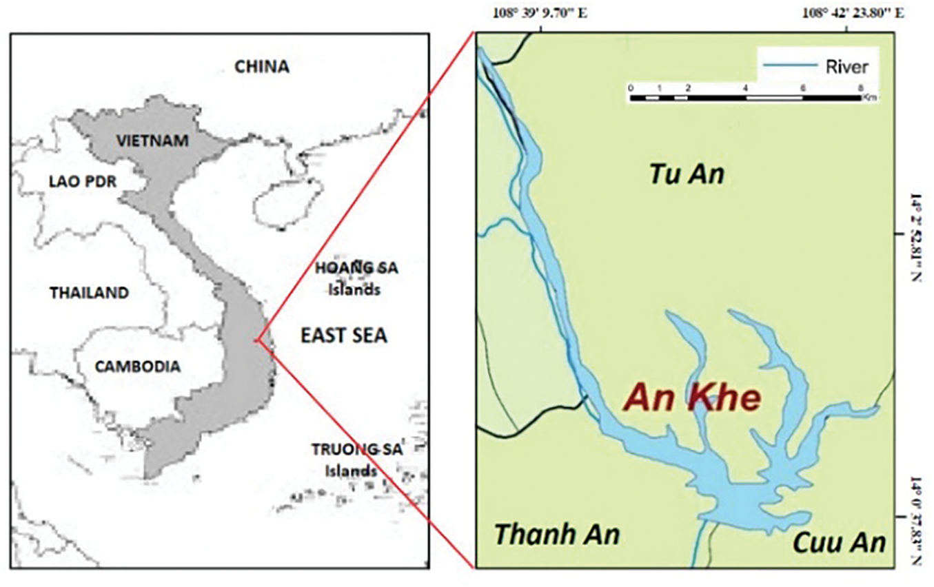
Figure 1: Geographical location map of the study area

where:

-   n is the number of data points.

-   qi is the actual value at the i-th data point.

-   qi^ is the predicted value at the i-th data point.

2.2 Proposed Methods

This part highlights each step in the proposed model. The main steps of the model are illustrated in Fig. 2.

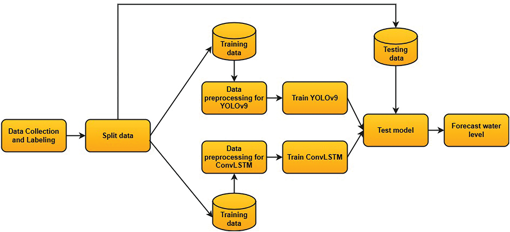
Figure 2: Framework of proposed model for water level prediction

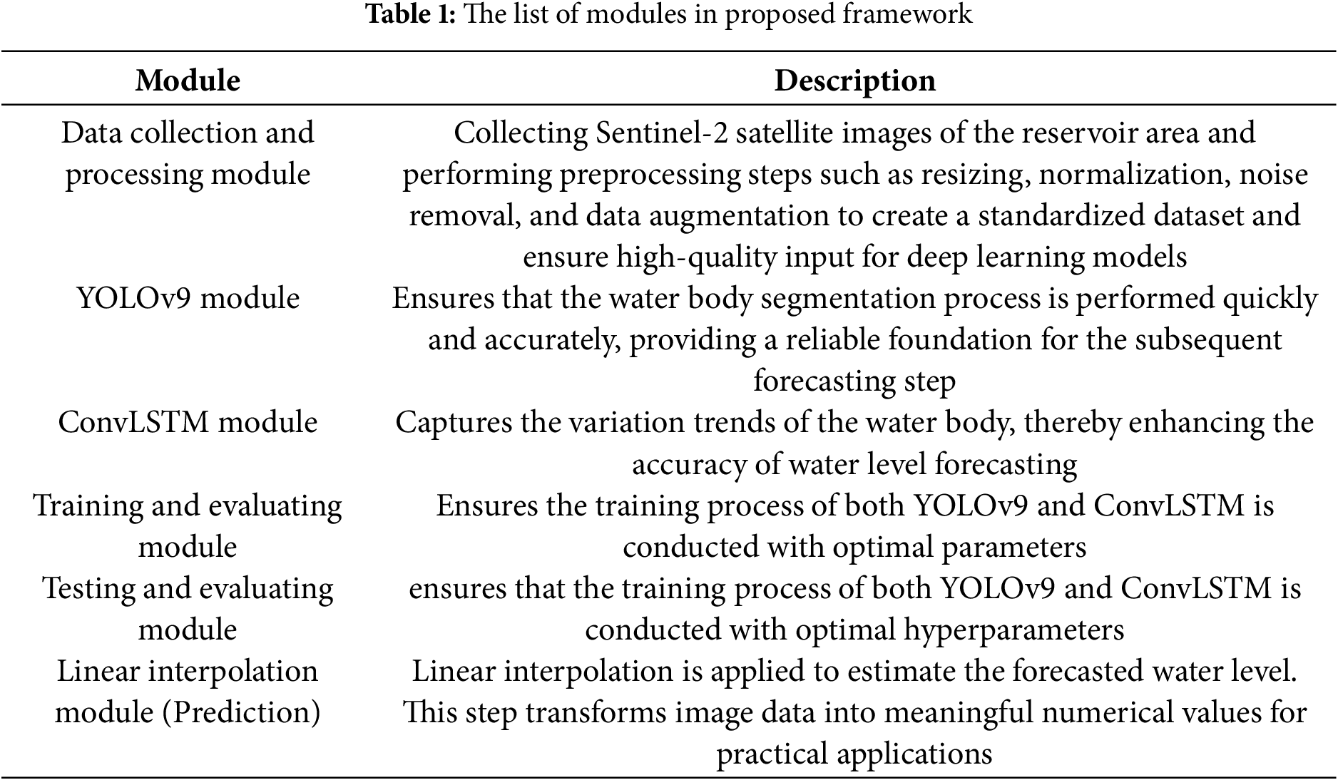
In the first stage, satellite images in the reservoir area are collected and labeled to obtain the input dataset. This dataset is split into two parts, including the training and testing sets. The training set is pre-proceeded and used to train YOLOv9 and ConvLSTM. The testing set is used to evaluate the proposed model. The model will generate predicted satellite images of the reservoir based on input images. After that, the surface area of reservoir is defined. Finally, the predicted water level is estimated using the linear interpolation method. The role of each module in the framework is given in Table 1 below.

2.2.1 Data Collection and Processing

This section describes the steps related to collection of Sentinel-2 satellite images for the study area illustrated in Fig. 3.

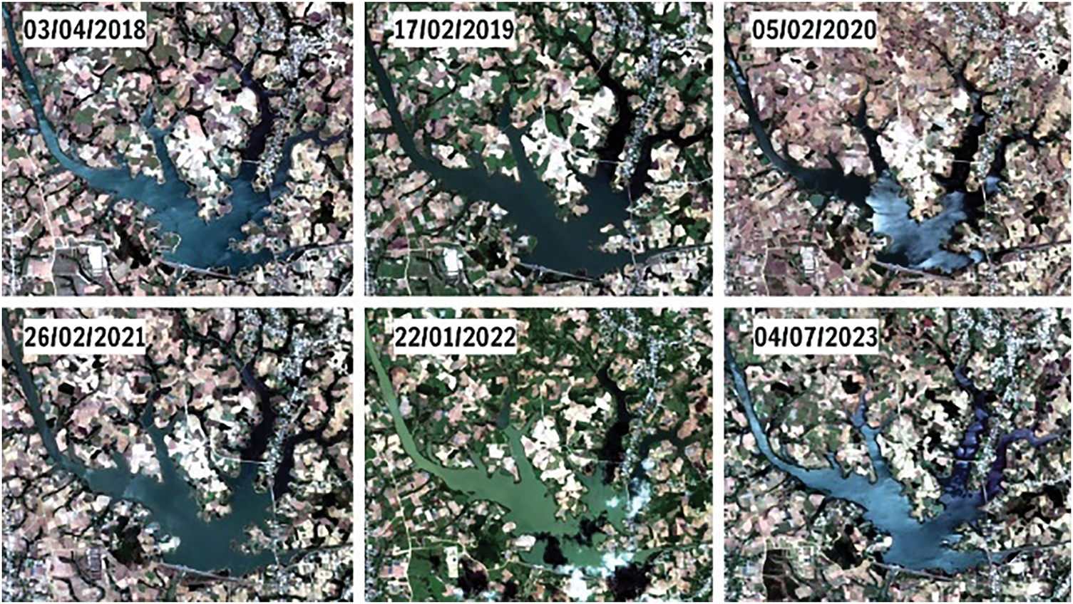
Figure 3: Examples of satellite images captured from An Khe

Data used in this research include the satellite images collected from the Copernicus program1 which belongs to the European Union’s space program. Images were collected from the Sentinel-2 satellite. Currently, the Copernicus program allows global users to access the open-source Open Hub1 free of charge. In this research, the following criteria were applied to retrieve satellite imagery from Copernicus: (i) the processing level was selected as Level 2A; the cloud cover threshold was set to <20%; (ii) the acquisition period was from 1 January 2018, to 31 December 2023; (iii) and the selected color bands were R4, G3, and B2. A total of 34 satellite images are included in this dataset. The satellite images are downloaded and extracted from the area of An Khe reservoir by using SNAP software2. The labeling process of images is performed by using consistent and suitable criteria to create a data set and its corresponding labels for each image. In the SNAP software, the following steps were used to get the coordinates of the reservoir area:

Step 1: Select the zip file and open it with the R4 (red), G3 (green) color bands, and B2 (blue). Zooming in the image displayed to the location of reservoir An Khe.

Step 2: Use a rectangular drawing tool to draw borders around An Khe reservoir area.

Step 3: Get the coordinates with WKT from Geometry and save it into temporary memory.

Step 4: Open GraphBuilder3, create subset (band 4, 3, 2), and save chart.

Step 5: Modify the polygon in the graph with the coordinates of the reservoir area.

Step 6: The final output is the Mygraph.xml file.

Data files are downloaded from the Copernicus website to SNAP software. The polygon coordinates were applied to the reservoir area, then the software automatically created the cut images in PNG format. The obtained images are from the area of An Khe reservoir. Fig. 3 presents several examples of the captured images.

Using the collected images, the next step is to label the water area of An Khe reservoir with the CVAT4 tool with the labeling environment for object segmentation for a task that includes 1 class (reservoir). Next, we upload the satellite image files and label them according to the following principles: The area to be segmented is the water area, characterized by continuously uniform colors. Place points to define the boundary between the water area and the non-water area. Assign these points to form a polygon that most accurately resembles the shape of the reservoir, as shown in Fig. 4. After labeling, the data is stored in MongoDB with two fields: ‘images’ and ‘labels’.

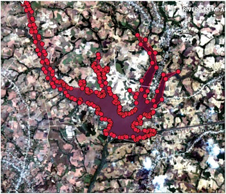
Figure 4: Satellite image after being labeled

2.2.2 Data Preprocessing

In this section, the data preprocessing steps for the proposed model is presented.

After being collected, the data has been organized in chronological order. This new dataset is used for preprocessing for each model, including YOLOv9 and ConvLSTM.

Data processing for the YOLOv9 model:

The data processing workflow for the YOLOv9 model is described in detail in Fig. 5. The steps are taken as follows: First from the collected image series will create the matrix of images and resize all images of 320 × 320 size to ensure consistency. Next, use Minimum Mean Square Error (MMSE) algorithm to restore image quality and reduce noise. Next, we use the methods of flipping horizontal images, flipping vertical images, flipping horizontally and flipping, turning the image clockwise, reversing the clock, and randomly cutting images to enhance the diversity of the object. After that, weadd the coordinates of the object in the label so that the object corresponds to the image after strengthening. Finally, we summarize the original images and images after strengthening into a set of training images for YOLOv9 and divide this data set into 3 data sections: train YOLOv9, val YOLOv9, test YOLOv9 with a ratio of 7:2:1.

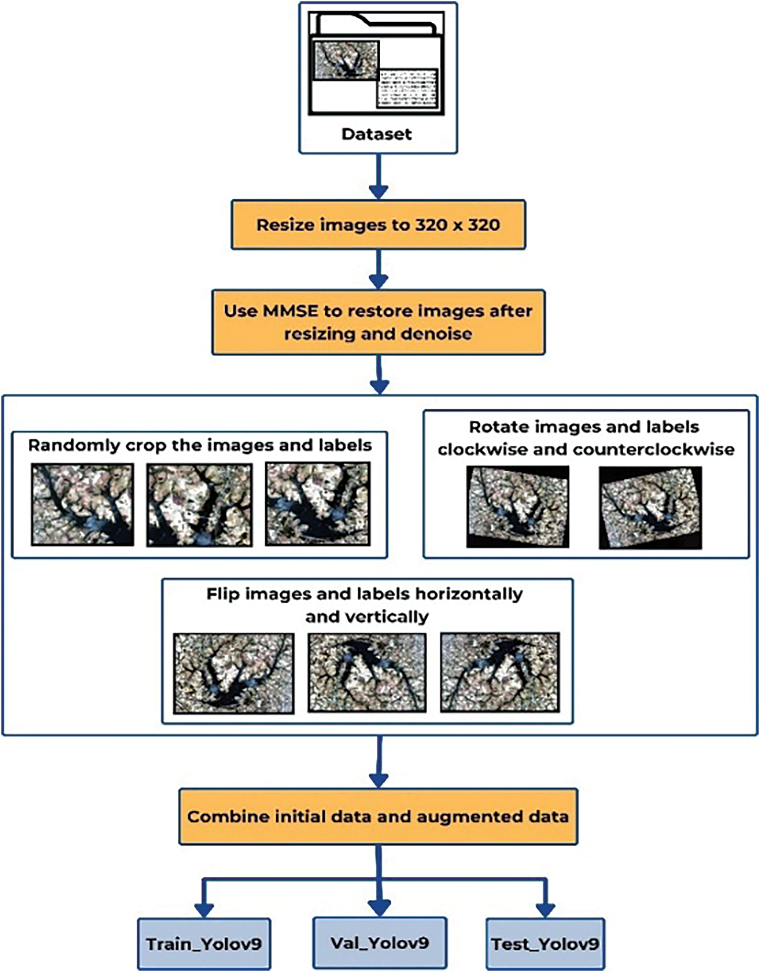
Figure 5: Data preprocessing for the YOLOv9 models

Data processing for ConvLSTM model:

The data processing procedure for the ConvLSTM model is detailed in Fig. 6. The sequential steps are as follows: First, from the collected image dataset, create a matrix of images and resize all images to 320 × 320 to ensure uniformity. Adjust the object coordinates in the labels to correspond to the objects in the resized images. Next, create a mask for the images with pixel values of 255 for regions containing the reservoir objects and pixel values ‘0’ for regions without reservoir objects, highlighting the features of the area of interest. Subsequently, for pixel points on the boundary, check the percentage of the reservoir object region at that point. If this percentage is larger than 50%, mark the pixel point as a reservoir object (value 255); otherwise mark it as not a reservoir object (value 0). Then, we perform monthly data statistics for the images over the years, identifying the number of images missing for each month in each year. We use the multi-point interpolation to augment the missing data for the months with missing images in the years, with the mathematical interpolation formula used from Eqs. (3)–(6) as follows:

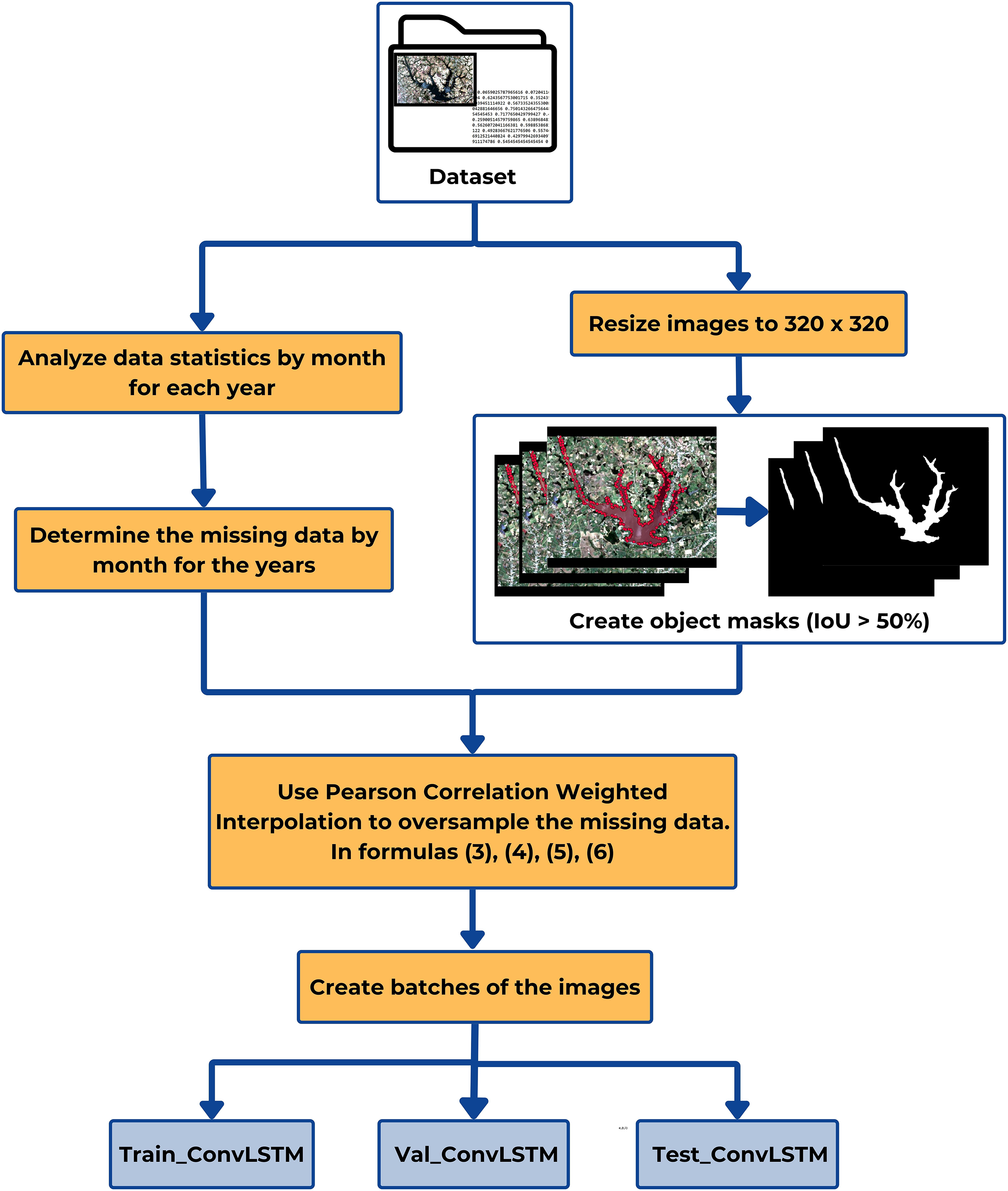
Figure 6: Data preprocessing for the ConvLSTM models

-   Calculate weights based on the Pearson correlation coefficients.

wi=corr(Ii,Ii+1)=cov(Ii,Ii+1)σIiσIi+1(3)

-   Calculate the images that need interpolation.

Iinterp=∑i=1n−1wi⋅Ii(4)

-   Normalize the interpolated images.

Iinterp=Iinterp∑i=1n−1wi(5)

-   Calculate the value range limits of the pixels.

Iinterp=clip(Iinterp,0,255)(6)

where:

-   Cov (Ii, Ii+1): The variance values of the i-th and (i + 1)-th images are needed for interpolation calculation.

-   σIi and σIi+1: The standard deviation of the pixel values of the i-th and (i + 1)-th images.

Finally, some slices of images and labels were created with a random time step from 3 to 10 and stride = 1 to prepare the data for the training process. Each batch includes 3 to 10 consecutive images; for example, with a time step of 4, it consists of images at times t − 3, t − 2, t − 1, and t, with the corresponding label at time t + 1. After creating batches and labeling the data, divide the data into three sets: train_ConvLSTM, val_ConvLSTM, and test_ConvLSTM with a ratio of 7:2:1.

2.2.3 Build and Train the YOLOv9 and ConvLSTM Model

The process of building and training the YOLOv9 model:

In this section, the YOLOv9 model will be built and trained. The process of building and training the model is described in Fig. 7. The YOLOv9 model is designed with three main components: Backbone, Neck, and Head. The Backbone utilizes convolutional layers, normalization, activation, and pooling to extract and process features from the data. Next, the Neck, with its FPN (Feature Pyramid Network) and PAN (Path Aggregation Network) architecture, aggregates features from the processed data of the Backbone. Finally, the Head is responsible for predicting bounding boxes, segmentation regions, object classes, and the confidence scores of the predicted areas.

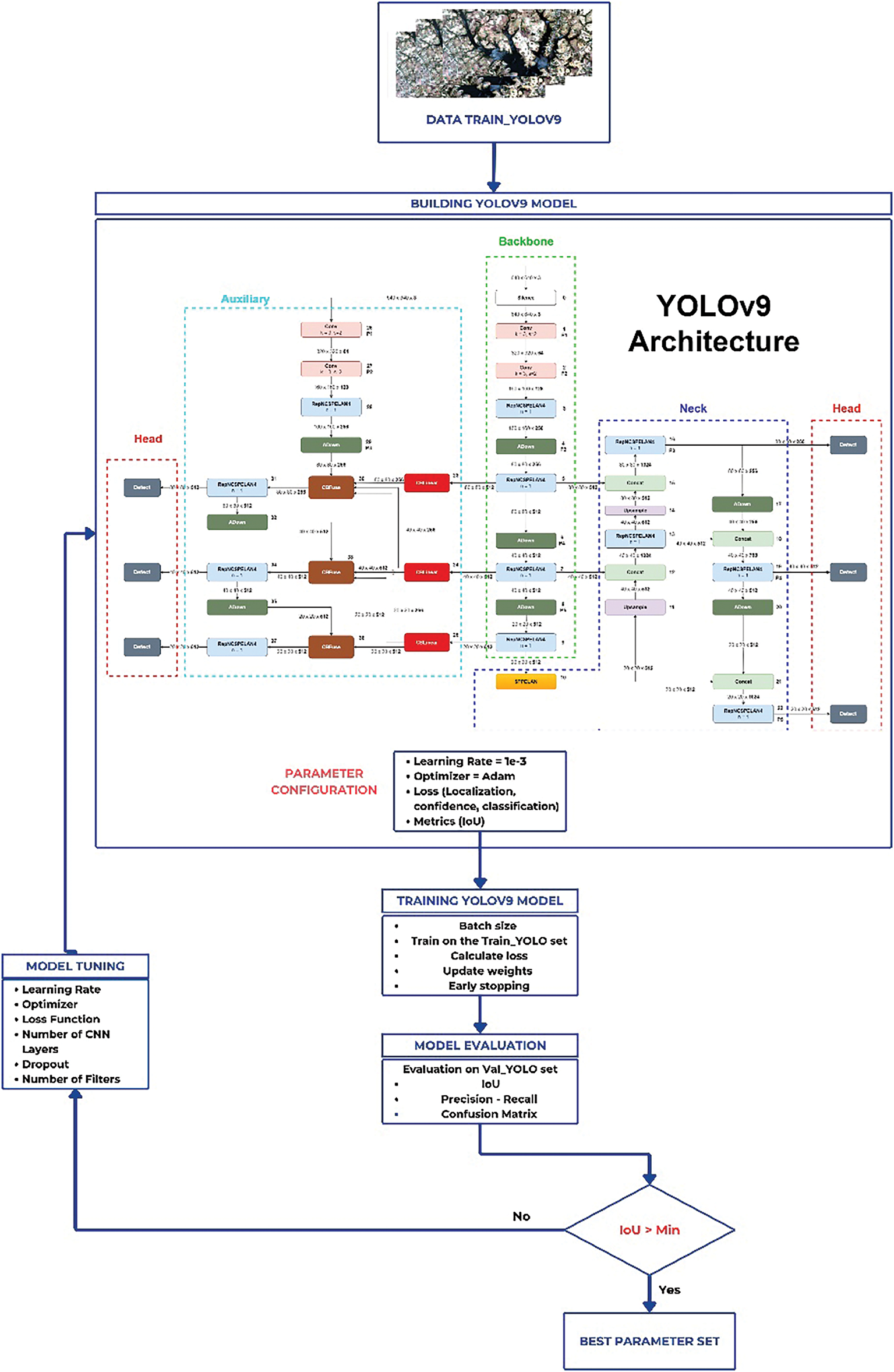
Figure 7: The training diagram of the YOLOv9 model

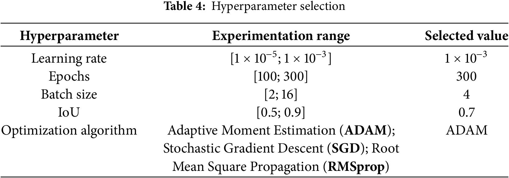
After completing the design of the YOLOv9 model, the parameters for the training process are set. The optimization algorithm used is Adam with a learning rate of ‘1 × 10−3’. The loss functions include localization loss, confidence loss, and classification loss. The YOLOv9 model will be trained on the train YOLOv9 dataset, with a batch size of 4300 epochs, and an IoU threshold of 0.7. Throughout the training process, the model computes the loss function and updates the weights after each epoch. Early stopping is employed: if the loss function does not improve significantly over 10 consecutive epochs, the training process will be halted.

Model evaluation is conducted on the val_YOLOv9 dataset using the following metrics: mAP (mean Average Precision), IoU (Intersection over Union), ‘Precision Recall’, and ‘Confusion Matrix’. After training, the model will be fine-tuned if it does not meet the condition IoU > Min. For the An Khe reservoir dataset, we choose Min = 90 (%). Adjustable parameters include the optimization algorithm, learning rate, loss function, number of convolutional layers, Dropout layers, and the number of filters in each convolutional layer. If the condition is met, the best model weights will be selected. If not, the parameters will be adjusted and training will be resumed. The experiments are conducted with various parameter sets and the best one that meets the model’s requirements is selected.

The process of building and training the ConvLSTM model:

In this section, the ConvLSTM model will be built and trained. The process of building and training the model is illustrated in Fig. 8. The ConvLSTM model consists of three ConvLSTM layers with specific parameters. The number of filters for each layer is 64, 32, and 1, respectively. Each layer has a stride of 1 and applies zero padding around the image after each feature extraction to maintain the input size. The activation function used in the model is ‘tanh’ function, which helps the model learn nonlinear relationships in the data. The model parameter configuration includes selecting the optimization algorithm and related parameters.

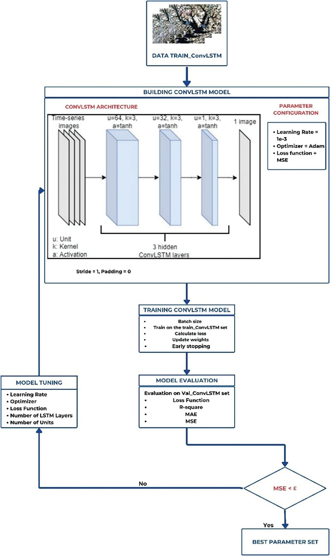
Figure 8: The training diagram of the ConvLSTM model

ADAM is used as the optimization algorithm with a learning rate as ‘1 × 10−3’. The loss function used is MSE (Mean Squared Error) to evaluate the model’s error during training. Training the ConvLSTM model involves a batch size of 4 and a total of 300 epochs. The model is trained on the train ConvLSTM dataset, with the loss function being computed and weights updated after each epoch. To prevent overfitting, early stopping is applied: if there is no significant improvement in the loss function over 10 consecutives epochs, the training process will be halted. After training, the model is evaluated on the val_ConvLSTM dataset using evaluation metrics such as R-squared, MAE (Mean Absolute Error), and MSE (Mean Squared Error). These metrics help assess the model’s performance with specific conditions: MSE < ε. For the An Khe reservoir dataset, we choose ε = 0.05. If these conditions are met, the weights of the best-performing algorithm, loss function, the number of ConvLSTM layers, and the number of units in each layer will be adjusted, and training will be resumed to improve the model.

2.2.4 Predicted Reservoir Water Level

The study collects technical design data of An Khe Reservoir5, including the relationship between water level, storage capacity, and surface area. Based on the interpretation results of the reservoir’s water surface area, combined with the established relationship, the water level of the reservoir can be determined. The following steps show the calculation of the reservoir area and forecast the water level.

Step 1: Count the number of pixels with a value of 255 (representing the reservoir) in the predicted mask image.

Step 2: Multiply the number of pixels from Step 1 by 100 m2 to calculate the area (since 1 pixel corresponds to 10 m × 10 m).

Step 3: Convert the area from square meters (m2) to square kilometers (km2) to match the units used in the An Khe hydroelectric reservoir data table.

Step 4: From the area value calculated in Step 3, compare it with the reference table to find the closest area range.

Step 5: Once the corresponding area range (Area) is identified, determine the corresponding water level range (Water Level).

Step 6: Use linear interpolation to calculate the reservoir water level, using Table 2 for interpolation. The linear interpolation formula is presented in Eq. (7):

y=(x−x1)∗(y2−y1)(x2−x1)+y1(7)

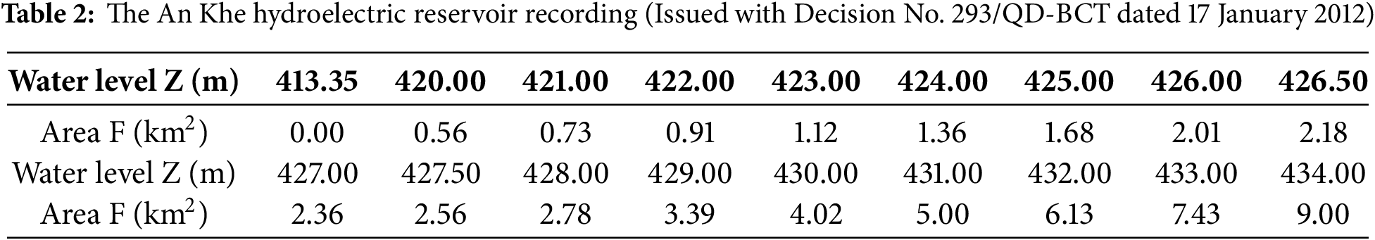
where, (y, y1, y2) is the reservoir water levels; (x, x1, x2) is the reservoir areas corresponding to the water levels; (y, y1, y2) and (x, x1, x2, y1, y2) are the known values, and y is the value to be determined.

Step 7: The final result is the reservoir water level based on the area calculated from the predicted mask image.

2.2.5 The Overall Process

After completing steps such as data collection, data preprocessing, and model training, the next step is to run the proposed model. The overall process of the model is detailed in Fig. 9. Using a time series of collected image data, data preprocessing is performed. This preprocessing step normalizes the input images by scaling pixel values to a range of ‘0’ to ‘1’, and then resizes the images to 320 × 320. These processed images are then fed into the YOLOv9 model for reservoir object region.

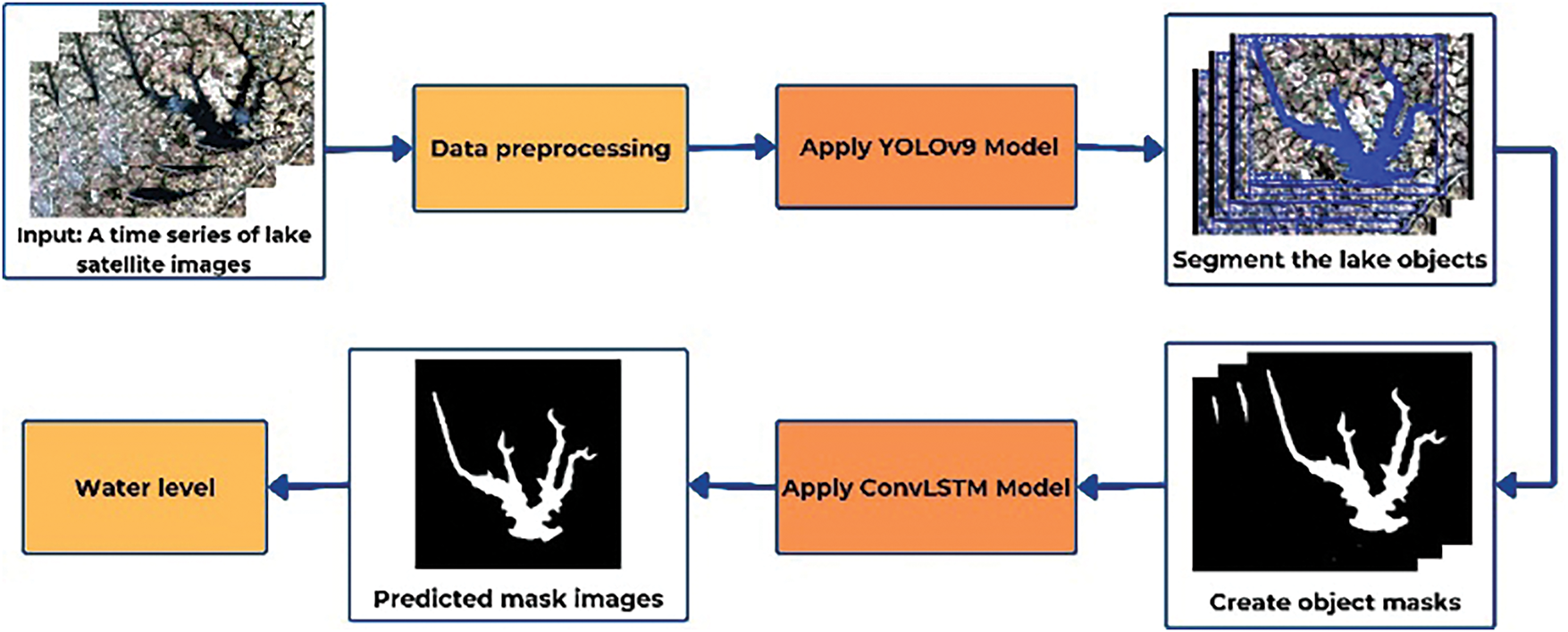
Figure 9: Illustration of steps in the proposed model

The sequence of images converted into object region masks is passed through the ConvLSTM model to forecast the reservoir mask for the next time step. Subsequently, the reservoir area and the forecasted water level are calculated according to Section 2.2.4. The model outputs the forecasted water level based on the input image sequence of the reservoir.

3  Results and Discussions

The experimental results presented in this section demonstrate that the proposed method (YOLOv9_ConvLSTM) outperforms other methods (SegNet_ConvLSTM, UNet_ConvLSTM) in terms of accuracy. The test scenarios were designed to compare these methods using the k-fold cross-validation, ensuring a comprehensive evaluation. Additionally, a two-way ANOVA was performed to analyze the variance in performance between the proposed method and the benchmark models, providing deeper insights into the model’s effectiveness.

3.1 Experimental Environments

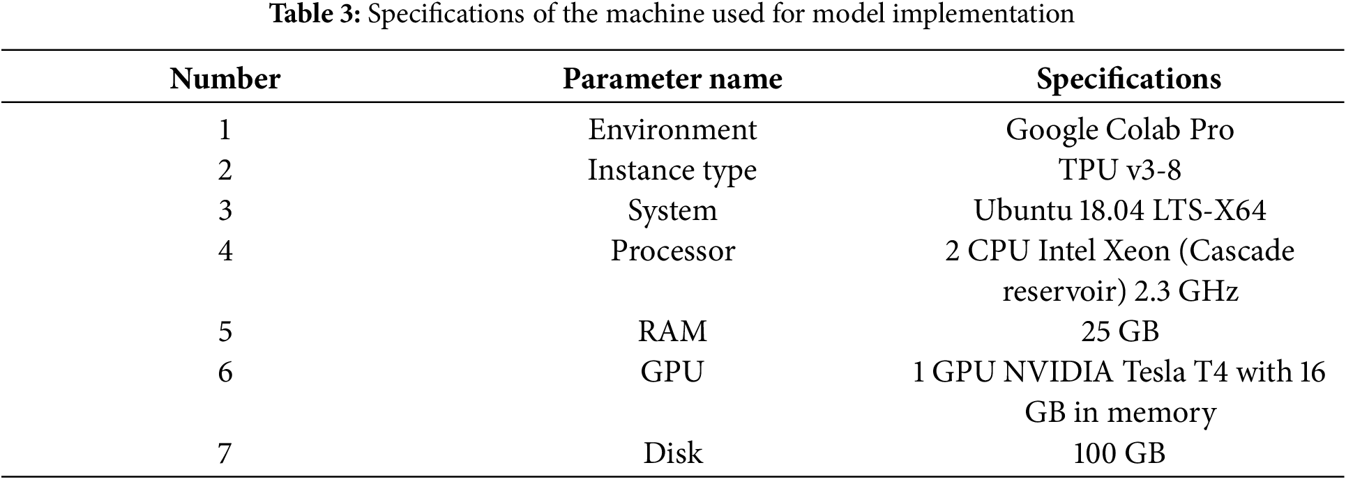
All experiments were conducted on Google Colab Pro with GPU support. The machine specifications are detailed in Table 3. In this experiment, satellite images of the An Khe reservoir region were used with each image representing a month from January to July 2024. Although only one image per month was available for the experiment, we designed reasonable scenarios to ensure that the quality of the proposed algorithm was not compromised. To compare the YOLOv9_ConvLSTM method with other reliable methods, we employed the k-fold cross-validation across three data-splitting scenarios as input for the forecasting methods.

Scenario 1: The input consists of 3 images

•   Use the original images from January, February, and March to forecast the image for April and compute the water level forecast for April.

•   Use the images from February, March, and the forecasted image for April as input to forecast the image for May and the water level forecast for May.

•   Use the original image from March and the forecasted images for April and May as input to forecast the image for June and the water level forecast for June.

•   Use the forecasted images for April, May, and June to forecast the image for July and the water level forecast for July.

Scenario 2: The input consists of 4 images

•   Use the original images from January, February, March, and April to forecast the image for May and compute the water level forecast for May.

•   Use the original images from February, March, April, and the forecasted image for May as input to forecast the image for June and the water level forecast for June.

•   Use the original images from March and April, along with the forecasted images for May and June, to predict the image for July and the water level forecast for July.

Scenario 3: The input consists of 5 images

•   Use the original images from January, February, March, April, and May to forecast the image for June and compute the water level forecast for June.

•   Use the original images from February, March, April, May, and the forecasted image for June as input to forecast the image for July and the water level forecast for July.

Hyperparameter setting: By implementing various values for hyperparameters, the optimized value is selected as in Table 4 below.

3.2 Experimental Results

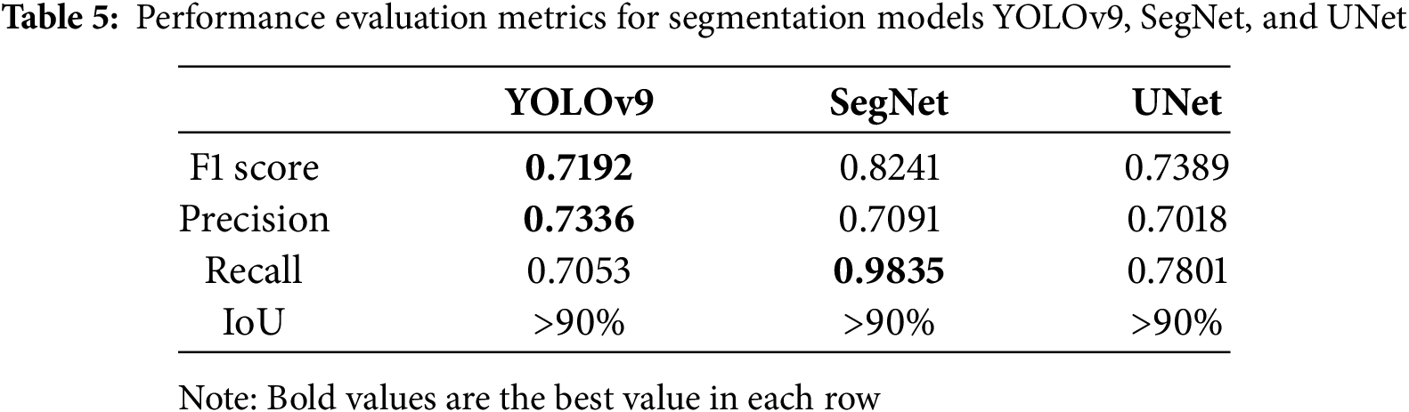
In this section, we describe the results of the proposed model compared to those of the other benchmark models. The training results of the YOLOv9, SegNet, and UNet image segmentation models are presented in Table 5, showcasing the performance evaluation metrics of each model. Although YOLOv9 does not outperform SegNet in the image segmentation phase, when integrated with the ConvLSTM forecasting network, the YOLOv9_ConvLSTM model demonstrates superior performance compared to the other models.

The results of empirical testing across three scenarios for the selected forecasting models, including Yolov9_ConvLSTM, SegNet_ConvLSTM, UNet_ ConvLSTM, are shown. The forecast results will be presented alongside the actual measured results at the corresponding time points in Figs. 10–12.

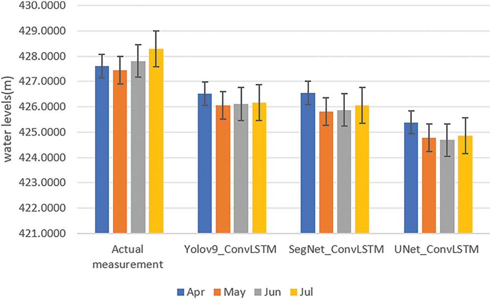
Figure 10: Results obtained from three models and actual water level under scenario 1

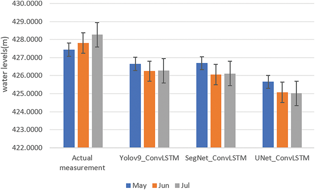
Figure 11: Results obtained from three models and actual water level under scenario 2

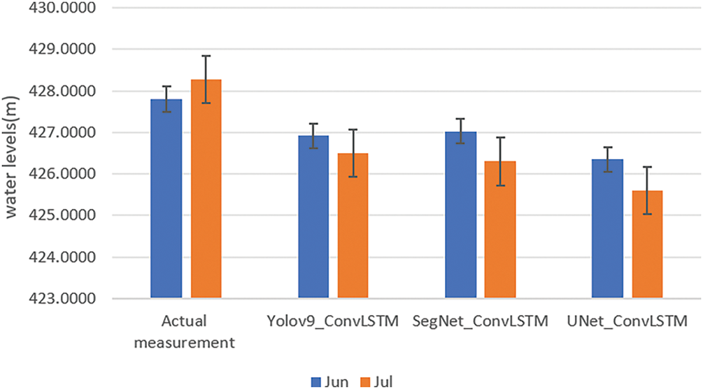
Figure 12: Results obtained from three models and actual water level under scenario 3

Based on Figs. 10–12, the YOLOv9_ConvLSTM model demonstrates higher forecasting accuracy compared to those of the SegNet-ConvLSTM and UNet-ConvLSTM models. Among them, the UNet-ConvLSTM model exhibits the lowest forecasting performance.

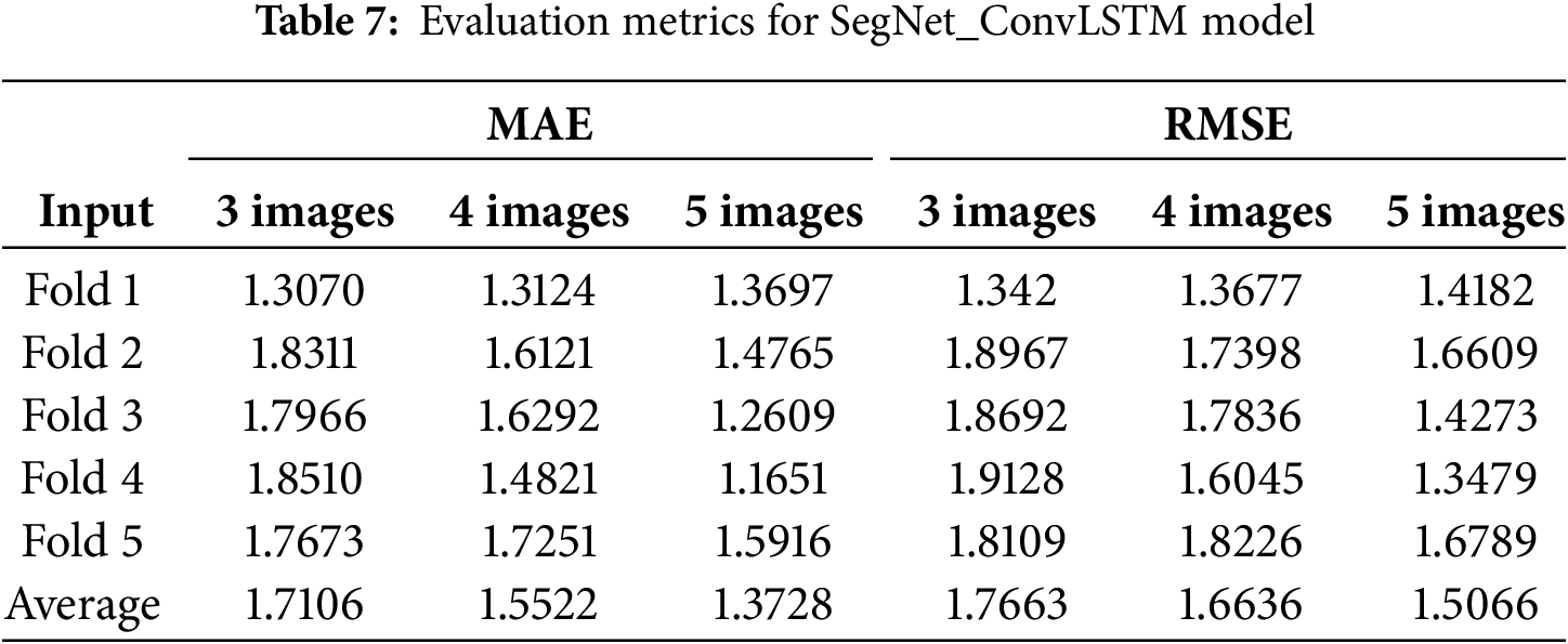
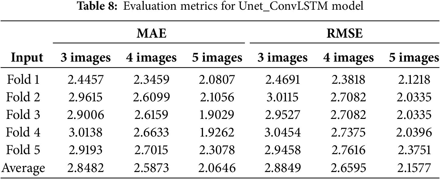
Apart from the comparison in Figs. 10–12, the evaluation metrics, including MAE and RMSE, are also calculated. After conducting experiments according to the described scenarios, the evaluation metrics of YOLOv9_ConvLSTM model, SegNet_ConvLSTM model and Unet_ConvLSTM model are given in Tables 6–8, respectively. In Tables 6–8, the authors present the MAE and RMSE evaluation results using a 5-fold approach for each scenario of the YOLOv9_ConvLSTM, SegNet_ConvLSTM, and Unet_ConvLSTM forecasting models. To ensure fair evaluation, we calculated the average value of the folds for each scenario, which is shown in the ‘Average’ row in Tables 6–8.

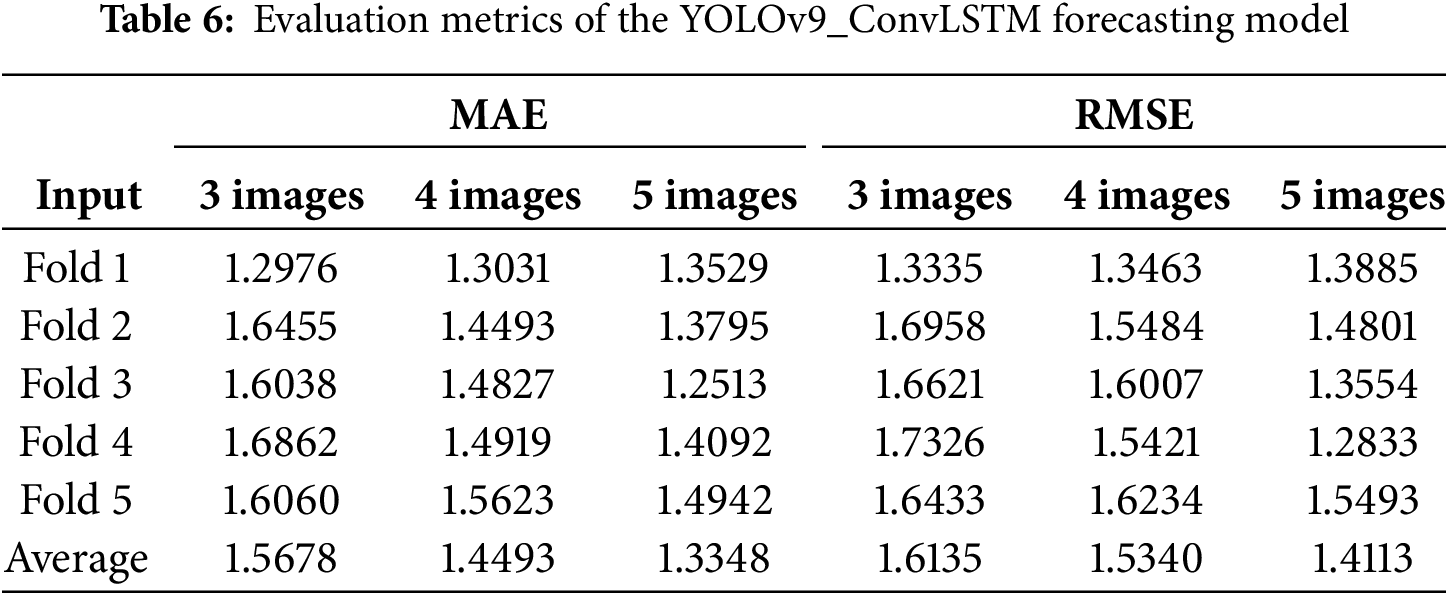
In Table 6, the ‘Average’ row for each scenario shows MAE values of 1.5678, 1.4493 and 1.3348, while the corresponding RMSE values are 1.6135, 1.5340 and 1.4113, respectively. A decreasing trend in both MAE and RMSE is observed, indicating that as the input images transition from original images to predicted images, the forecasting accuracy of the model gradually declines.

In Table 7, the ‘Average’ row for each scenario shows MAE values of 1.7106, 1.5522, and 1.3728, while the corresponding RMSE values are 1.7663, 1.6636, and 1.5066, respectively. A decreasing trend in both MAE and RMSE is observed, indicating that as the input images transition from original images to predicted images, the forecasting accuracy of the model gradually declines.

In Table 8, the ‘Average’ row for each scenario shows MAE values of 2.8482, 2.5873 and 2.0646, while the corresponding RMSE values are 2.8849, 2.6595 and 2.1577, respectively. A decreasing trend in both MAE and RMSE is observed, indicating that as the input images transition from original images to predicted images, the forecasting accuracy of the model gradually declines. Table 9 summarizes the average MAE and RMSE values for each fold of the YOLOv9-ConvLSTM, SegNet-ConvLSTM, and Unet-ConvLSTM forecasting models.

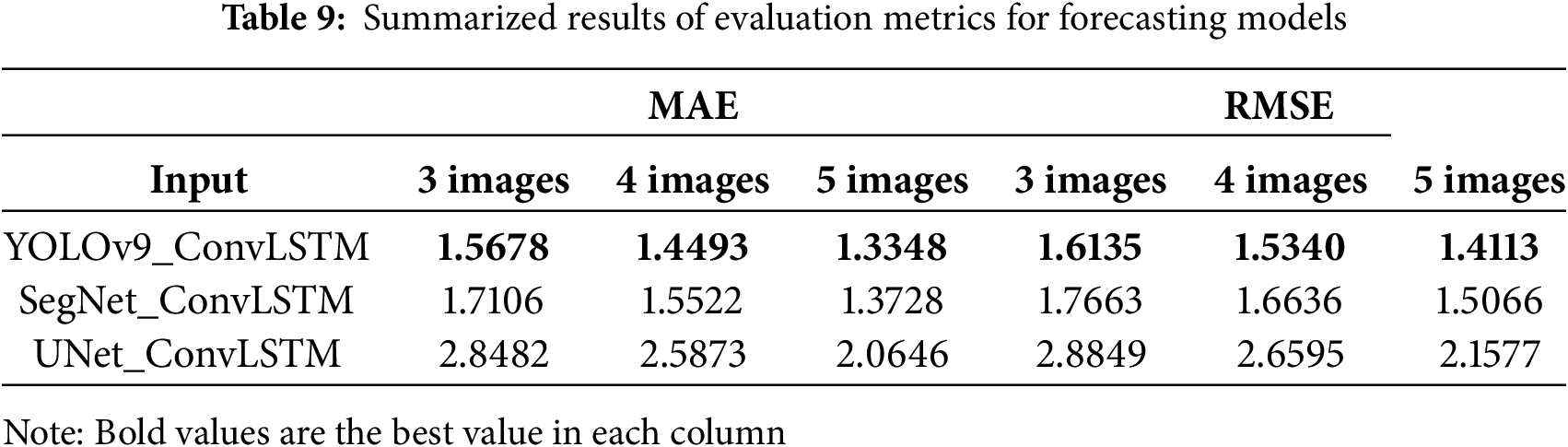
The results in Table 9 indicate that the proposed YOLOv9-ConvLSTM model achieves the lowest MAE and RMSE values across all three scenarios. Specifically, the MAE values are 1.5678, 1.4493, and 1.3348, while the RMSE values are 1.6135, 1.5340, and 1.4113, respectively. This demonstrates that the YOLOv9-ConvLSTM model provides more accurate forecasting results compared to the benchmark models.

3.3 ANOVA Analysis

A two-way ANOVA with a significance level of α = 0.05 is utilized to evaluate our proposed approach (YOLOv9_ConvLSTM) across multiple scenarios and compare it to other related methods (SegNet_ConvLSTM and Unet_ConvLSTM). The two null hypotheses H0 and H1 are stated below:

-   H0: There are no statistically significant differences in performance between the groups of models

-   H1: There are no statistically significant differences in performance between the groups of scenarios

ANOVA analyses are performed regarding the values of MAE and RMSE measurements. The analysis results in MAE are shown in Table 10.

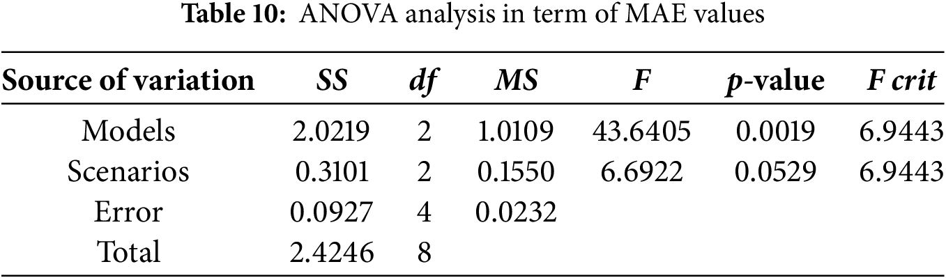
As in Table 10, by the groups of models, the p-value is less than the significance level (0.0019 vs. 0.05). It means that hypothesis H0 is rejected. In other words, the performance in groups of models is significantly different via MAE. By the groups of scenarios, the p-value is greater than alpha (0.0529 vs. 0.05). Thus, the hypothesis H1 is accepted. This indicates that the mean of MAE in various scenarios is not significantly different. To identify models being different, the post-hoc tests need to be performed by the pairs of models. The analysis results in RMSE are shown in Table 11 below.

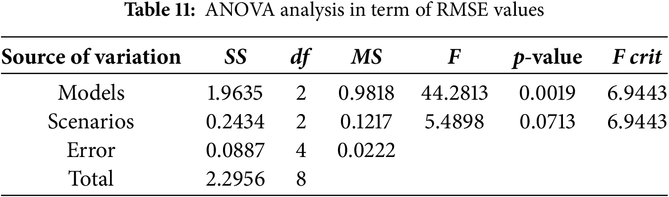
The results in Table 11 are same as those in Table 10. It means that H0 is rejected and H1 is accepted in terms of RMSE. Moreover, the small error values in two of these tables (0.0232 and 0.0222) show that random fluctuations are minimal and the models have explained the variance in the data well.

Post-hoc tests among three pairs of models use Bonferroni correction calculated by α/3 = 0.05/3 = 0.0167. The results are summarized in Table 12.

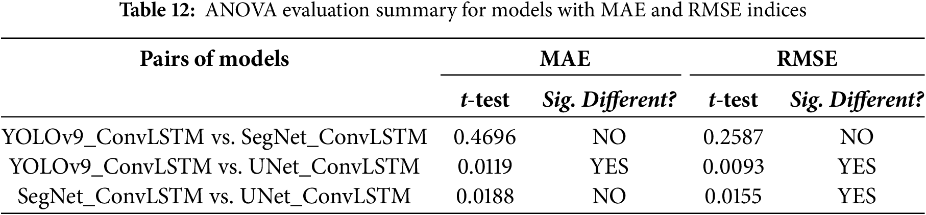
Based on the results in Table 12, YOLOv9_ConvLSTM and UNet_ConvLSTM have significant differences via MAE. Regarding RMSE, there are differences between YOLOv9_ConvLSTM and SegNet_ConvLSTM with UNet_ConvLSTM. In this measure, YOLOv9_ConvLSTM and SegNet_ConvLSTM results are of the same performance.

3.4 Discussions

The proposed method effectively integrates deep learning and remote sensing techniques for reservoir water level forecasting using Sentinel-2 satellite imagery. Specifically, the model employs the YOLOv9 network for reservoir segmentation, ConvLSTM to model spatiotemporal relationships, and linear interpolation to estimate the forecasted water level.

To evaluate the performance of the proposed YOLOv9_ConvLSTM model, this study implemented other advanced image segmentation methods, including SegNet and UNet, which were then integrated with ConvLSTM to construct hybrid models SegNet_ConvLSTM and UNet_ConvLSTM for validation. The experimental results, presented in Table 9, indicate that the YOLOv9_ConvLSTM model outperforms the other approaches.

Additionally, as a baseline comparison, we also implemented a standalone ConvLSTM model on the same dataset, with the comparative results detailed in Table 13. These findings demonstrate that incorporating an image segmentation stage before forecasting the next frame using ConvLSTM significantly enhances model performance, highlighting the critical role of combining spatial and temporal processing in image forecasting tasks.

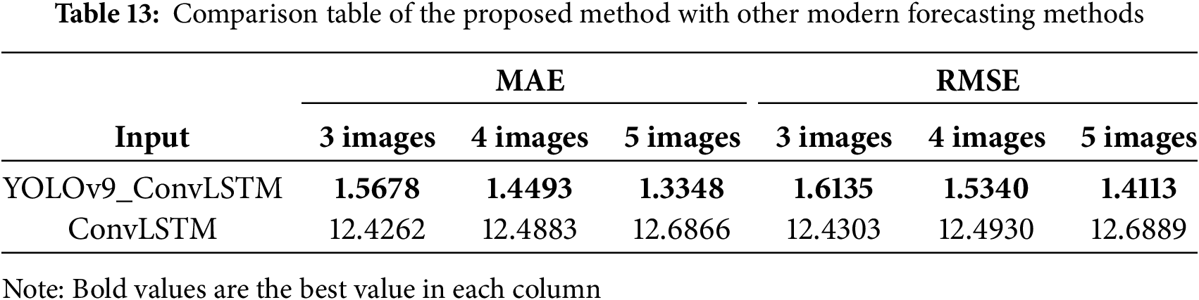
As shown in Table 13, the MAE and RMSE values of the proposed model exhibit a reduction of over 87% compared to those of the original ConvLSTM model across all test scenarios, demonstrating the superior effectiveness of the proposed approach.

A key advantage of this approach is leveraging free satellite imagery, optimizing costs, and enabling broad applicability in water resource management, particularly in regions lacking in-situ measurement systems. However, the model still has some certain limitations. Firstly, processing large-scale satellite image datasets requires significant computational resources, posing challenges when scaling up forecasting across multiple reservoirs or extending the prediction horizon. Secondly, the model’s accuracy may be affected by environmental noise, particularly cloud cover, which degrades the quality of input images.

4  Conclusion

In this study, we focused on developing a unique approach for estimating reservoir water levels using free Sentinel-2 satellite images. The primary contributions of this study include (i) introducing a process for acquiring and labeling Sentinel 2 images of the An Khe reservoir region; (ii) proposing a hybrid model in which YOLOv9 network is used to segment the reservoir area and generate masks for the labeled reservoir region from the satellite images, ConvLSTM network is applied to predict the next mask of the reservoir region and linear interpolation is selected to estimate the forecasted water level; (iii) implementing the proposed forecasting model and benchmarked it against SegNet_ConvLSTM and Unet_ConvLSTM models to validate its performance. The results demonstrated that the proposed model achieved better accuracy.

However, the proposed model has some drawbacks, such as high computational time when dealing with large input image datasets. For further research directions, the developing forecasting models based on Sentinel 2 remote sensing data combined with operational reservoir data such as inflow and rainfall will be considered. Moreover, utilizing optimization algorithms to fine-tune the parameters in the YOLOv9_ConvLSTM model to improve the performance is also studied.

Future research should explore the usage of additional hydrological and meteorological data, such as inflow, outflow, and precipitation, to enhance forecasting accuracy. Moreover, adopting advanced optimization techniques, including hyperparameter tuning using Bayesian optimization or reinforcement learning, could improve the performance of the YOLOv9_ConvLSTM model, reducing computational costs and enhancing generalization capability.

Overall, this study demonstrates the potential of deep learning models combined with satellite imagery for reservoir water level forecasting, offering a modern and more efficient alternative to traditional hydrological models.

Acknowledgement: The authors appreciate the support from Prof. Le Hoang Son from the Artificial Intelligence Research Center (AIRC) and the leaders and staff members from Institute of Information Technology (IOIT).

Funding Statement: This research is funded by International School, Vietnam National University, Hanoi (VNU-IS) under project number CS.2023-10.

Author Contributions: Concept: Tran Kim Chau, Tran Manh Tuan, Hoang Thi Minh Chau; Methodology: Tran Thi Ngan, Nguyen Long Giang, Hoang Thi Minh Chau; Software: Tran Manh Tuan, Hoang Thi Minh Chau; Validation: Tran Thi Ngan, Nguyen Long Giang; Data curation: Tran Thi Ngan, Hoang Thi Minh Chau; Writing—original draft preparation: Tran Manh Tuan, Hoang Thi Minh Chau; Writing—review and editing: Tran Thi Ngan, Tran Kim Chau. All authors reviewed the results and approved the final version of the manuscript.

Availability of Data and Materials: Not applicable.

Ethics Approval: Not applicable.

Conflicts of Interest: The authors declare no conflicts of interest to report regarding the present study.

1https://dataspace.copernicus.eu/ (accessed on 1 January 2025).

2https://step.esa.int/main/download/snap-download/ (accessed on 1 January 2025).

3https://docs.yworks.com/yfiles-html/dguide/graph_builder/graph_builder-GraphBuilder.html (accessed on 1 January 2025).

4https://www.cvat.ai/ (accessed on 1 January 2025).

5https://en.evn.com.vn/d6/news/An-Khe-Ka-Nak-hydropower-plant-ensures-water-supply-for-Ba-River-downstream-basin-in-the-dry-season-66-163-2813.aspx (accessed on 1 January 2025).

References

1. Yaseen ZM, Sulaiman SO, Deo RC, Chau KW. An enhanced extreme learning machine model for river flow forecasting: state-of-the-art, practical applications in water resource engineering area and future research direction. J Hydrol. 2019;569(2):387–408. doi:10.1016/j.jhydrol.2018.11.069. [Google Scholar] [CrossRef]

2. Xu ZX, Li JY. Short-term inflow forecasting using an artificial neural network model. Hydrol Process. 2002;16(12):2423–39. doi:10.1002/hyp.1013. [Google Scholar] [CrossRef]

3. Moosavi V, Vafakhah M, Shirmohammadi B, Behnia N. A wavelet-ANFIS hybrid model for groundwater level forecasting for different prediction periods. Water Resour Manag. 2013;27(5):1301–21. doi:10.1007/s11269-012-0239-2. [Google Scholar] [CrossRef]

4. Nagappan M, Gopalakrishnan V, Alagappan M. Prediction of reference evapotranspiration for irrigation scheduling using machine learning. Hydrol Sci J. 2020;65(16):2669–77. doi:10.1080/02626667.2020.1830996. [Google Scholar] [CrossRef]

5. Deka PC. Support vector machine applications in the field of hydrology: a review. Appl Soft Comput. 2014;19(3):372–86. doi:10.1016/j.asoc.2014.02.002. [Google Scholar] [CrossRef]

6. Altunkaynak A. Forecasting surface water level fluctuations of lake van by artificial neural networks. Water Resour Manag. 2007;21(2):399–408. doi:10.1007/s11269-006-9022-6. [Google Scholar] [CrossRef]

7. Alvisi S, Mascellani G, Franchini M, Bárdossy A. Water level forecasting through fuzzy logic and artificial neural network approaches. Hydrol Earth Syst Sci. 2006;10(1):1–17. doi:10.5194/hess-10-1-2006. [Google Scholar] [CrossRef]

8. Ali Ghorbani M, Khatibi R, Aytek A, Makarynskyy O, Shiri J. Sea water level forecasting using genetic programming and comparing the performance with artificial neural networks. Comput Geosci. 2010;36(5):620–7. doi:10.1016/j.cageo.2009.09.014. [Google Scholar] [CrossRef]

9. Hipni A, El-shafie A, Najah A, Karim OA, Hussain A, Mukhlisin M. Daily forecasting of dam water levels: comparing a support vector machine (SVM) model with adaptive neuro fuzzy inference system (ANFIS). Water Resour Manag. 2013;27(10):3803–23. doi:10.1007/s11269-013-0382-4. [Google Scholar] [CrossRef]

10. Mosavi A, Ozturk P, Chau KW. Flood prediction using machine learning models: literature review. Water. 2018;10(11):1536. doi:10.3390/w10111536. [Google Scholar] [CrossRef]

11. Páliz Larrea P, Zapata-Ríos X, Campozano Parra L. Application of neural network models and ANFIS for water level forecasting of the salve faccha dam in the Andean zone in northern Ecuador. Water. 2021;13(15):2011. doi:10.3390/w13152011. [Google Scholar] [CrossRef]

12. Shiri J, Shamshirband S, Kisi O, Karimi S, Bateni SM, Hosseini Nezhad SH, et al. Prediction of water-level in the urmia lake using the extreme learning machine approach. Water Resour Manag. 2016;30(14):5217–29. doi:10.1007/s11269-016-1480-x. [Google Scholar] [CrossRef]

13. Yan P, Zhang Z, Hou Q, Lei X, Liu Y, Wang H. A novel IBAS-ELM model for prediction of water levels in front of pumping stations. J Hydrol. 2023;616(8):128810. doi:10.1016/j.jhydrol.2022.128810. [Google Scholar] [CrossRef]

14. Deo RC, Şahin M. An extreme learning machine model for the simulation of monthly mean streamflow water level in eastern Queensland. Environ Monit Assess. 2016;188(2):90. doi:10.1007/s10661-016-5094-9. [Google Scholar] [PubMed] [CrossRef]

15. Ul Islam S, Jan S, Waheed A, Mehmood G, Zareei M, Alanazi F. Land-cover classification and its impact on Peshawar’s land surface temperature using remote sensing. Comput Mater Contin. 2022;70(2):4123–45. doi:10.32604/cmc.2022.019226. [Google Scholar] [CrossRef]

16. Song S, Zhang R, Hu M, Huang F. Fine-grained ship recognition based on visible and near-infrared multimodal remote sensing images: dataset, methodology and evaluation. Comput Mater Contin. 2024;79(3):5243. doi:10.32604/cmc.2024.050879. [Google Scholar] [CrossRef]

17. Singh A, Vyas V. A review on remote sensing application in river ecosystem evaluation. Spatial Inf Res. 2022;30(6):759–72. doi:10.1007/s41324-022-00470-5. [Google Scholar] [CrossRef]

18. Wang L, Tang Q, Li W, Wang X, Zhang H, Xu J, et al. Remote sensing image analysis and cyanobacterial bloom prediction method based on ACL3D-Pix2Pix. Desalin Water Treat. 2023;297:138–59. [Google Scholar]

19. Avisse N, Tilmant A, Müller MF, Zhang H. Monitoring small reservoirs’ storage with satellite remote sensing in inaccessible areas. Hydrol Earth Syst Sci. 2017;21(12):6445–59. doi:10.5194/hess-21-6445-2017. [Google Scholar] [CrossRef]

20. Schumann G, Di Baldassarre G, Bates PD. The utility of spaceborne radar to render flood inundation maps based on multialgorithm ensembles. IEEE Trans Geosci Remote Sens. 2009;47(8):2801–7. doi:10.1109/TGRS.2009.2017937. [Google Scholar] [CrossRef]

21. Lan W, Yang T, Chen Q, Zhang S, Dong Y, Zhou H, et al. Multiview subspace clustering via low-rank symmetric affinity graph. IEEE Trans Neural Netw Learn Syst. 2024;35(8):11382–95. doi:10.1109/TNNLS.2023.3260258. [Google Scholar] [PubMed] [CrossRef]

22. Wieland M, Martinis S, Kiefl R, Gstaiger V. Semantic segmentation of water bodies in very high-resolution satellite and aerial images. Remote Sens Environ. 2023;287:113452. doi:10.1016/j.rse.2023.113452. [Google Scholar] [CrossRef]

23. Ronneberger O, Fischer P, Brox T. U-Net: convolutional networks for biomedical image segmentation. In: Medical Image Computing and Computer-Assisted Intervention—MICCAI 2015: 18th International Conference; 2015 Oct 5–9; Munich, Germany. Cham, Switzerland: Springer International Publishing; 2015. p. 234–41. doi:10.1007/978-3-319-24574-4_28. [Google Scholar] [CrossRef]

24. Nie X, Duan M, Ding H, Hu B, Wong EK. Attention mask R-CNN for ship detection and segmentation from remote sensing images. IEEE Access. 2020;8:9325–34. [Google Scholar]

25. Weng L, Xu Y, Xia M, Zhang Y, Liu J, Xu Y. Water areas segmentation from remote sensing images using a separable residual SegNet network. ISPRS Int J Geo Inf. 2020;9(4):256. doi:10.3390/ijgi9040256. [Google Scholar] [CrossRef]

26. Aziz F, Saputri DUE. Efficient skin lesion detection using YOLOv9 network. MEDINFTech. 2024;2(1):11–5. doi:10.37034/medinftech.v2i1.30. [Google Scholar] [CrossRef]

27. Ahmad R, Yang B, Ettlin G, Berger A, Rodríguez-Bocca P. A machine-learning based ConvLSTM architecture for NDVI forecasting. Int Trans Operational Res. 2023;30(4):2025–48. doi:10.1111/itor.12887. [Google Scholar] [CrossRef]

28. Zheng L, Lu W, Zhou Q. Weather image-based short-term dense wind speed forecast with a ConvLSTM-LSTM deep learning model. Build Environ. 2023;239(5):110446. doi:10.1016/j.buildenv.2023.110446. [Google Scholar] [CrossRef]

29. Farooque G, Xiao L, Yang J, Sargano AB. Hyperspectral image classification via a novel spectral-spatial 3D ConvLSTM-CNN. Remote Sens. 2021;13(21):4348. doi:10.3390/rs13214348. [Google Scholar] [CrossRef]

30. Wang L, Li W, Wang X, Xu J, Zhao Z, Yu J, et al. Remote sensing image prediction of water environment based on 3D CNN and ConvLSTM. Geosci Remote Sens. 2022;5(1):28–39. [Google Scholar]

31. Ghorbanzadeh O, Rostamzadeh H, Blaschke T, Gholaminia K, Aryal J. A new GIS-based data mining technique using an adaptive neuro-fuzzy inference system (ANFIS) and k-fold cross-validation approach for land subsidence susceptibility mapping. Nat Hazards. 2018;94(2):497–517. doi:10.1007/s11069-018-3449-y. [Google Scholar] [CrossRef]

32. Sawyer SF. Analysis of variance: the fundamental concepts. J Man Manip Ther. 2009;17(2):27E–38E. doi:10.1179/jmt.2009.17.2.27E. [Google Scholar] [CrossRef]