Rolling Bearing Fault Diagnosis Based on 1D Convolutional Neural Network and Kolmogorov–Arnold Network for Industrial Internet

1  Introduction

Rolling bearings are critical mechanical components widely used in various industrial applications. Their performance directly influences the operational stability and safety of machinery, making rolling bearing fault diagnosis a crucial area of research in mechanical fault detection [1]. Early detection of bearing faults can effectively prevent equipment failures, reduce maintenance costs, and extend equipment lifespan [2]. Traditional fault diagnosis methods, including time-domain analysis, frequency-domain analysis, and wavelet transform, have proven effective under simple operating conditions. However, they exhibit significant limitations when applied to complex conditions, particularly with regard to signal variations due to load fluctuations [3].

With advancements in artificial intelligence and deep learning, deep neural networks, particularly Convolutional Neural Networks (CNNs), have become the standard for fault diagnosis. Recent developments have led to high-accuracy intelligent fault diagnosis methods for aero-engine bearings and generalized fault diagnosis frameworks based on phase entropy, demonstrating promising results. For example, Wang et al. proposed a method integrating refined composite multiscale phase entropy (RCMPhE) with Bonobo Optimization Support Vector Machine (SVM), improving fault recognition accuracy by 28.97% compared to existing techniques, even with just five training samples per fault type. This method achieved 100% accuracy in small-sample fault diagnosis [4]. Additionally, Wang introduced a generalized fault diagnosis framework utilizing refined time-shift multi-scale phase entropy and Twin SVM, which achieved over 99.51% accuracy with only five training samples, outperforming nine other models and showcasing strong generalization capabilities [5]. Traditional deep learning methods often rely on training data collected under specific load conditions, limiting their adaptability when load changes occur. In real-world industrial environments, machine operating loads fluctuate with changing working conditions, leading to significant variations in vibration signals. This introduces a domain adaptation problem in machine learning, where the distribution of data in the source domain (e.g., data collected under one load condition) differs from that in the target domain (data collected under another load condition). Solving this problem—training a model on source domain data to effectively diagnose target domain signals—has become a critical challenge in fault diagnosis [6,7].

The domain adaptation problem is particularly prominent in rolling bearing fault diagnosis. Signal changes caused by load variation are typically nonlinear and highly complex, which makes traditional deep learning methods, such as CNNs and Long Short-Term Memory (LSTM) networks, struggle with cross-load diagnosis [8]. Although techniques like transfer learning and adversarial training have been widely applied to solve domain adaptation problems, existing methods still face significant challenges when dealing with highly nonlinear signal variations.

In recent years, many researchers have proposed deep learning-based solutions to address the issue of load variation in rolling bearing fault diagnosis. For example, Qiao proposed a dual-input CNN-LSTM model for rolling bearing fault diagnosis, utilizing both time and frequency domain features for enhanced fault classification [9]. Alex developed an intelligent fault diagnosis method using a novel dual-path RNN-WDCNN model, which combines recurrent and convolutional neural networks to diagnose rolling element bearing faults from raw vibration data [10]. The scholar proposed a weakly supervised one-dimensional convolutional neural network for diagnosing permanent magnet synchronous motors, effectively identifying motor states and eccentric effects under varying conditions [11]. While these methods alleviate the impact of load variation on model performance to some extent, they still suffer from several issues:

Insufficient Nonlinear Feature Modeling: Traditional CNN models can extract low-level features from signals, but they have limited capability in modeling the complex nonlinear features present in the signals;

Poor Adaptability across Loads: Existing methods typically train models using data from the same load conditions, and they exhibit poor adaptability when faced with changes in load-induced signal differences;

Scarcity of Target Domain Data: Many domain adaptation methods require large amounts of labeled target domain data, but obtaining labeled data from the target domain is often costly and difficult in industrial settings.

To address these challenges, this paper proposes a novel fault diagnosis method (CNN-1D-KAN) for rolling bearings based on the combination of 1D Convolutional Neural Network (1D-CNN) and Kolmogorov–Arnold Network (KAN). Compared with traditional CNNs, 1D-CNN is more efficient for handling one-dimensional time-series data, making it ideal for fault diagnosis using vibration signals. KAN is a nonlinear modeling technique based on Kolmogorov complexity theory, which can capture high-order nonlinear features of signals [12]. In the KAN model, multi-layer nonlinear transformations are used to effectively model the complex dynamic processes of signals, thus improving the model’s adaptability to complex signal variations.

2  Related Work

2.1 Kolmogorov–Arnold Network (KAN)

In the rapidly advancing field of neural networks, Kolmogorov–Arnold Network (KAN) offers a novel approach to network architecture, grounded in the Kolmogorov–Arnold representation theorem [13]. According to this theorem, any continuous multivariate function can be expressed as a composition of univariate functions combined with addition operations. This fundamental principle distinguishes KANs from conventional Multi-Layer Perceptron (MLP).

The essence of KAN lies in its distinctive architecture. In contrast to traditional MLP, which employs fixed activation functions at the nodes, KANs utilize learnable activation functions on the network edges. This fundamental shift from static to dynamic activation functions involves replacing conventional linear weight matrices with adaptive spline functions, which are parameterized and optimized throughout the training process. This enables a more flexible and responsive model that can dynamically adjust to complex data patterns. More specifically, the Kolmogorov–Arnold representation theorem asserts that a multivariate function f(x1,⋯,xn) can be expressed as:

f(x1,⋯,xn)=∑q=12n+1Φq(∑p=1nϕq,p(xp))(1)

Φq and ϕq,p are learnable univariate functions that collaboratively manage the network’s input-output mapping. This configuration enables KAN to process high-dimensional data by decomposing its complexity into simpler, one-dimensional operations, effectively avoiding the curse of dimensionality that often challenges traditional MLP. Additionally, KAN utilizes splines as activation functions on the network connections.

Spline Activation Functions: In the network, each connection is governed by a spline function, as defined by the following formula:

spline(t)=∑i=1kBi(t)ci(2)

where ci are the coefficients learned during training, and Bi(t) represents the spline basis functions.

Network Function Representation: The network is characterized by the following function:

f(x)=∑j=1majσj(wjTx+bj)(3)

where σj denotes the spline-based activation functions, wj represents the input weights, bj are the biases, and aj refers to the output weights.

2.2 Difference between KAN and MLP

KAN and MLP are both neural network structures, but they have some significant differences in design concepts, structures, and application backgrounds [14]. Table 1 is a summary of the comparison between the two:

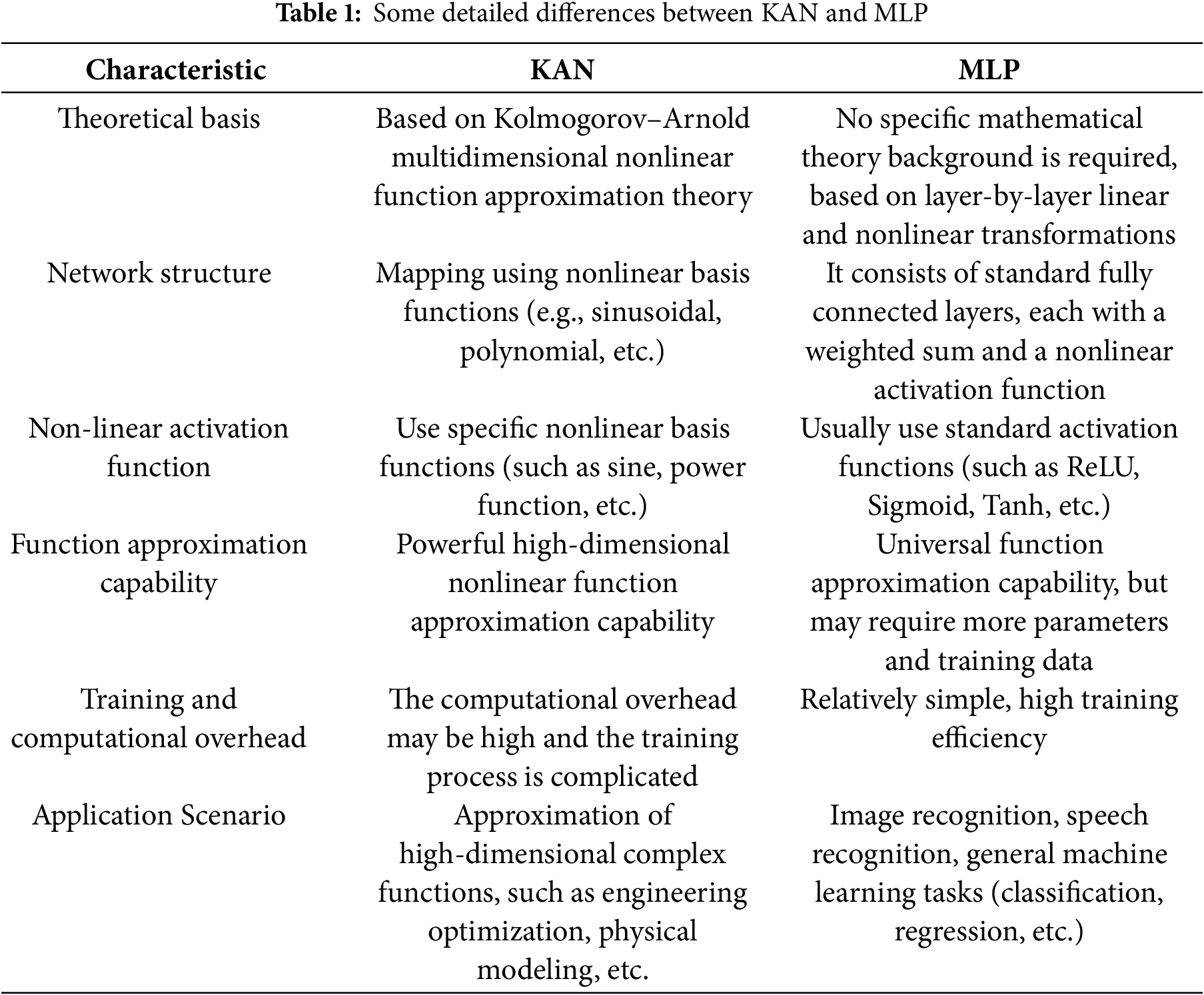
In conclusion, KAN has theoretical advantages in approximating complex high-dimensional nonlinear functions and is suitable for scenarios that require efficient representation of complex nonlinear relationships; while MLP is a general and easy-to-implement neural network suitable for handling conventional supervised learning tasks, especially classification and regression problems.

3  Methodology

3.1 Description of Variable Load Problem

The variation in workload is a common occurrence in mechanical systems. When the load changes, the signals measured by sensors also undergo variations. Fig. 1 presents the diagnostic signals under different loads, with the normalized inner-race fault size set to 0.007 inches. As shown in Fig. 1, the number of features in the vibration signal, as well as their amplitude, fluctuate differently under various load conditions. Additionally, the fluctuation periods and phase differences vary significantly. These discrepancies may lead to the classifier’s inability to correctly categorize the extracted features, thereby reducing the identification accuracy of the intelligent diagnostic system.

Figure 1: Diagnostic signal of inner-race fault size of 0.007 inch under different loads: (a) 0 HP; (b) 1 HP; (c) 2 HP; (d) 3 HP

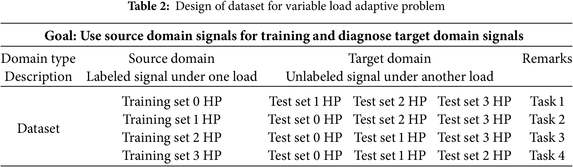
Therefore, applying a machine learning model trained with data from a specific load to perform fault diagnosis on vibration signals under varying loads holds significant practical value. In this experiment, vibration signals under 0, 1, 2, and 3 HP loads are used to train the CNN-1D-KAN model, while the signals from the remaining three load conditions serve as the test set. The specific description of the variable load adaptation problem is provided in Table 2.

3.2 Proposed CNN-1D-KAN Model

In this work, we propose the one-dimensional convolutional neural network and Kolmogorov–Arnold Network (CNN-1D-KAN) model by redefining the CNN model by replacing fully connected layers (FCLs) with KanLinear layer. The complete fault diagnosis flowchart is shown in Fig. 2.

Figure 2: The flowchart of fault diagnosis

The CNN-1D-KAN model, depicted in Fig. 3, is specifically designed for processing one-dimensional input data, making it well-suited for tabular classification tasks. The architecture begins with an input layer, followed by a first convolutional layer (Conv1D) that has 1 input channel for extracting feature numbers and 32 output channels for initial feature extraction. This is followed by a ReLU (Rectified Linear Unit) activation layer to introduce non-linearity, and then a max-pooling layer to reduce the dimensionality of the input data. The second stage consists of a second Conv1D layer with 32 input channels and 64 output channels, followed by another ReLU activation layer and a max-pooling layer. In the third stage, a third Conv1D layer with 64 input channels and 128 output channels is applied, again followed by a ReLU activation layer and a max-pooling layer. Subsequently, an adaptive average pooling layer is introduced, which does not require predefined settings for the pooling kernel size, padding, or stride. This layer reduces the feature map size to a single dimension, preparing the data for the subsequent layer. The core innovation of the model lies in the KANLinear layer, which replaces the traditional fully connected layers (FCL) and processes the 128-dimensional input to generate the final output. In the structure design of the KANLinear layer, the grid size is set to 5, the order of the piecewise polynomial is set to 3, the scaling noise is set to 0.1, the base scaling is set to 1.0, the piecewise polynomial scaling is set to 1.0, and independent piecewise polynomial scaling is enabled. The base activation function is set to Sigmoid Linear Unit, the grid adjustment parameter is set to 0.02, and the grid range is set to [−1, 1]. By replacing the last fully connected layer of the traditional 1D-CNN with the KANLinear layer, this innovation allows this layer to combine KAN’s nonlinear processing capabilities, complex function approximation capabilities, and the simplicity of linear transformation. Traditional neural networks require multiple layers of stacking to approximate complex functions, while KANLinear achieves more efficient expression through adaptive activation functions, thereby reducing dependence on deep networks and improving training efficiency. This replacement may enable the model to more flexibly handle complex relationships between features while maintaining efficient calculations, further enhance the model’s feature representation capabilities, and reduce model complexity. The KANLinear layer, through its unique mechanism, better integrates and transforms features from different levels, thereby helping the model make a more accurate trade-off between global and local information.

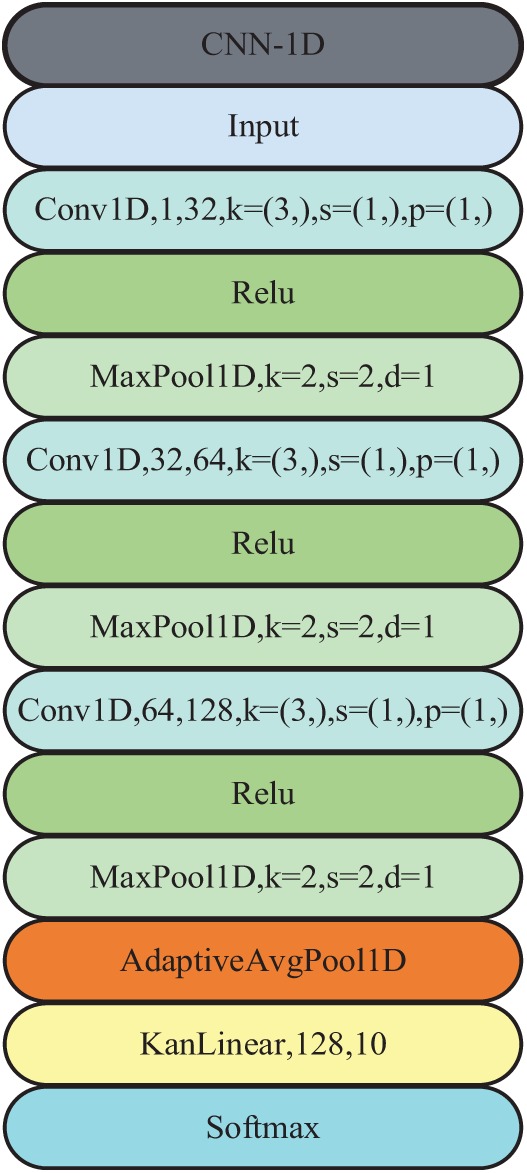
Figure 3: Framework of the proposed CNN-1D-KAN model, it consists of 13 layers such as input, Conv1D, Relu, MaxPool1D, AdaptiveAvgPool1D, KanLinear, and softmax layer. k represents kernel_size, s represents stride, d represents dilation and p represents padding

4  Experimental and Analysis of Results

This experiment uses the Pytorch deep learning framework with a hardware environment of 13th Gen Intel® core (TM) i9-13900k 3.0 Hz CPU, GeForce RTX 4090 GPU, windows 11 operating system, and PyCharm 2023.1.4 (Professional Edition).

4.1 Dataset

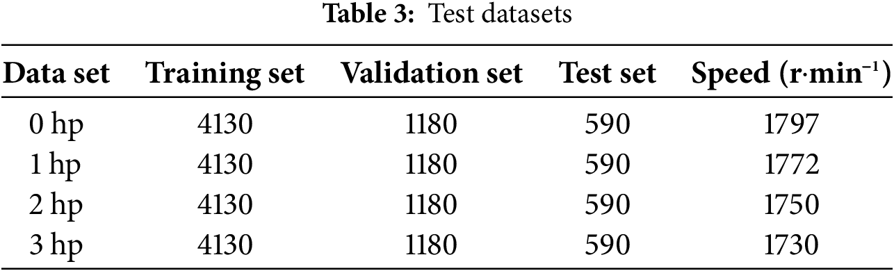
To verify the effectiveness of the CNN-1D-KAN model, the experiment uses the rolling bearing vibration data of Case Western Reserve University (CWRU) as the data set for this experiment. The CWRU data set has been widely used in bearing fault diagnosis. The experimental platform consists of sensors, power testers, motors, etc. The vibration signals of the fan end and the bearing drive end are collected at 48 and 12 kHz. Each fault data set has a different fault diameter. There are four different motor loads under each fault diameter: 0, 1, 2, and 3 hp. There are three types of faults under each load, namely rolling element, outer ring, and inner ring faults. The outer ring fault can be divided into three positions according to the position: 3 o’clock, 6 o’clock, and 12 o’clock. This experiment uses the drive end data of SKF-6205 with a frequency of 12 Hz. According to the size of the fault diameter, fault position and normal data, the experimental data is divided into 10 categories. The experiment uses data under four load conditions to train the model. Since the length of each data file is inconsistent, in order to ensure the consistency of the length, according to the principle of the barrel effect, the data file with the shortest length of 121,265 is selected as the unified total data length. Take 1024 consecutive data points as a sample. To avoid overfitting caused by too little data, the method of data overlapping sampling [15] is used for data enhancement. The calculation sformula is as follows:

N=L−L1L1∗(1−D)+1

where N is the number of samples obtained; L is the total length of the data; L1 is the length of a single sample data; D is the overlap rate, which is 0.8 here. According to the above formula, 5900 samples are obtained for each data set, and the ratio of training set, validation set and test set is set to 7:2:1. The specific data is shown in Table 3.

4.2 Evaluation Metrics

The performance of the model in bearing fault diagnosis is evaluated using several key metrics, which offer valuable insights into its effectiveness in detecting faults. These metrics include accuracy, precision, recall, and the F1 score.

Accuracy measures the proportion of correct predictions out of all predictions. It is calculated as follows:

Accuracy=TP+TNTN+TP+FP+FN(4)

where TP denotes true positives, TN represents true negatives, FP stands for false positives, and FN refers to false negatives.

Precision refers to the proportion of true positive predictions out of all positive predictions. It quantifies the model’s accuracy in identifying positive instances and is defined as follows:

Precision=TPFP+TP(5)

Recall, also known as the true positive rate, measures the model’s ability to correctly identify all actual positive instances. It is calculated using the following formula:

Recall=TPFN+TP(6)

The F1 score offers a balanced evaluation by combining both precision and recall. As the harmonic mean of these two metrics, it provides a comprehensive assessment of the model’s performance. The F1 score is calculated using the following formula:

F1score=2×Precision∗RecallPrecision+Recall(7)

Macro avg calculates the macro average of these indicators. Without considering the difference in the number of samples for each category, sum up the indicators for each category and divide by the total number of categories N to obtain the average value of each indicator. The specific calculation method is as follows:

macro avg of precision=precision1+⋯+precisionNN(8)

macro avg of recall=recall1+⋯+recallNN(9)

macro avg of F1score=F1score1+⋯+F1scoreNN(10)

where precisionia2+b2 represent the proportion of samples correctly predicted as class i out of all samples predicted as class i, recalli represent the proportion of samples correctly predicted as class i out of all actual instances of class i, and F1scorei denote the weighted harmonic mean of precision and recall, which provides a comprehensive consideration of both metrics.

4.3 Parameter Settings of CNN-1D-KAN

When building a convolutional neural network, choosing appropriate parameters according to different tasks can greatly improve the model’s performance. During the model training process, the training set is usually divided into multiple batch sizes and input into the model for training in sequence. However, if the batch size is too large, the generalization performance of the model will be reduced, and if it is too small, the model will not converge easily. Therefore, in the process of building CNN-1D-KAN, this paper selects the batch size parameter that affects the model accuracy and training speed, and sets it to 16, 32, 64, and 128 for experiments. The model accuracy results are shown in Fig. 4a. When the Batchsize is 16 and 32, the model accuracy is higher in the initial training stage and tends to converge when the training reaches the 17th epoch. Although the model accuracy of the model with Batchsize of 16 is higher than that of the model with Batchsize of 32 when epoch is less than 13, the two are basically consistent after the 13th epoch; at the same time, considering the impact of Batchsize on the model training speed, as shown in Fig. 4b, the training time of the model with Batchsize of 16 is 150 s, while the training time of the model with Batchsize of 32 is 133 s. Considering the factors of model accuracy and training speed, this paper selects Batchsize of 32.

Figure 4: Effect of batch size on (a) model accuracy and (b) training speed

4.4 Design of Comparative Experimental Model

To demonstrate the effectiveness of the CNN-1D-KAN model, it is compared with four other intelligent fault recognition models: CNN-1D, KAN, KAN Convolutions (KANConv), and Multilayer Perceptron (MLP). Specifically, the CNN-1D model is obtained by replacing the second-to-last layer, KanLinear, of the CNN-1D-KAN model with a fully connected layer, while keeping the other settings consistent with the CNN-1D-KAN model. The MLP model consists of three fully connected layers. The KAN model comprises three KanLinear layers. The KANConv model primarily consists of three KAN convolutional layers, four max-pooling layers, one Flatten layer, and two fully connected layers. To avoid the random bias of the experimental results, all experiments used the 5-fold cross-validation method. The Adam optimizer was used for training, the learning rate was 0.0001, the training was carried out for 20 epochs, and the Batchsize was 32. The architectural details of these four comparison models are shown in Fig. 5.

Figure 5: Architectural information of four comparative experimental models. o represents the target output size and n represents the number of convolutions to be applied

4.5 Fault Diagnosis Results under the Same Load and Comparison with Other Methods

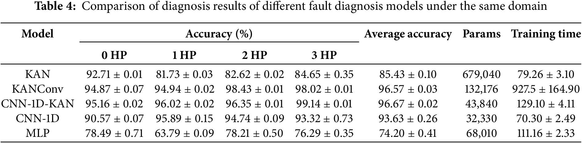
As shown in Table 4, CNN-1D-KAN demonstrates outstanding performance across all load conditions, particularly under 3 HP, where it achieves an accuracy of 99.14%, significantly outperforming other models. This indicates that CNN-1D-KAN is particularly effective at identifying fault features under high-load conditions. In contrast, the KAN model exhibits lower accuracy under 1, 2, and 3 HP, highlighting its limited adaptability to varying load conditions. The average accuracy of CNN-1D-KAN is 96.67%, the highest among all models. It maintains stable performance across different load conditions (from 0 to 3 HP), demonstrating robustness in handling diverse fault scenarios. This is in contrast to the other models, where performance fluctuates significantly under different load conditions. CNN-1D-KAN has a relatively small parameter count of 43,840, compared to KAN (679,040) and KANConv (132,176). Despite its superior accuracy, CNN-1D-KAN is more parameter-efficient, making it computationally more efficient. This results in a better trade-off between model complexity and performance. CNN-1D-KAN requires 129.10 ± 4.11 s to train, which is slightly longer than CNN-1D (70.30 ± 2.49 s) but much shorter than KANConv (927.5 ± 164.90 s). While CNN-1D-KAN has a higher training time than CNN-1D, it still provides a good balance between training efficiency and performance. It is far more efficient than KANConv in terms of training time while still achieving superior accuracy. The performance of CNN-1D and MLP is notably inferior to CNN-1D-KAN. Specifically, CNN-1D performs well under 1 HP but lags behind CNN-1D-KAN in terms of overall accuracy and robustness under higher load conditions (2 and 3 HP). MLP exhibits the lowest accuracy across all load conditions, with a maximum of only 63.79% at 1 HP. Its performance is inconsistent, indicating that MLP is not suitable for handling the complex time-series data and load variations present in the CWRU dataset.

4.6 Bearing Diagnostic Results and Analysis across Different Load Domains

In this section, we provide a detailed comparative analysis of five fault diagnosis models—KAN, KANConv, CNN-1D-KAN, CNN-1D, and MLP—under domain adaptation scenarios. Specifically, we evaluate the models’ performance in the source domain of 0 HP and their adaptation to target domains of 1, 2, and 3 HP, as shown in Table 5 and Fig. 6a. The evaluation metrics used for comparison include accuracy, precision, recall, and F1 score.

Figure 6: Comparison of adaptability results of five models under different load migration tasks. (a) the source domain is 0 HP and the target domain is 1, 2, and 3 HP; (b) the source domain is 1 HP and the target domain is 0, 2, and 3 HP; (c) the source domain is 2 HP and the target domain is 0, 1, and 3 HP; (d) the source domain is 3 HP and the target domain is 0, 1, and 2 HP

The KAN model demonstrates relatively poor performance, particularly in the 1 and 2 HP domains, with accuracy and F1 scores below 53%. While the performance slightly improves in the 3 HP domain, it remains limited in generalization and domain adaptation, as evidenced by its low recall values (e.g., 46.91% in 3 HP). The low recall suggests that KAN struggles to correctly identify faulty samples, leading to a higher false negative rate. The KANConv model significantly improves over KAN, particularly in 2 and 3 HP domains, with accuracy exceeding 72% and F1 scores surpassing 80%. The increase in precision and recall demonstrates that the addition of convolutional layers enhances feature extraction and reduces misclassification. However, its performance still falls short of CNN-1D-KAN, indicating that while it extracts better hierarchical features than KAN, it lacks attention-based domain adaptation mechanisms, leading to inconsistent recall across different loads. The CNN-1D-KAN model is the top performer across all domains, achieving over 85% accuracy in 2 and 3 HP and excelling in 1 HP with 89.06% accuracy. More importantly, it maintains consistently high precision (above 86%), recall, and F1 scores, demonstrating its superior ability to generalize across varying load conditions. The synergy between CNN-1D for spatial-temporal feature extraction and KAN for domain adaptation allows it to handle complex load variations with higher robustness. The CNN-1D model achieves the highest accuracy (92.71%) and F1 score (92.55%) in the 1 HP domain, surpassing all models in this scenario. However, its performance declines in the 2 and 3 HP domains, where it falls behind CNN-1D-KAN. The lack of KAN-based domain adaptation results in lower recall, indicating a drop in its ability to generalize across different operating conditions. Finally, the MLP model exhibits the weakest performance, particularly in the 1 HP domain (accuracy 35.59%, F1 score 38.76%). Its failure to capture temporal dependencies and load-specific variations leads to poor recall and inconsistent classification performance. The model’s reliance on fully connected layers makes it ineffective for handling time-series fault data, further emphasizing the importance of convolutional and knowledge-based models in this field.

As shown in Table 6 and Fig. 6b, the models were trained on the 1 HP dataset and evaluated on the 0, 2, and 3 HP datasets. A comprehensive analysis of accuracy, precision, recall, and F1 score reveals significant differences in generalization ability across models. The KAN model demonstrates moderate performance in the 0 and 3 HP target domains, while achieving relatively higher accuracy in the 2 HP domain. Despite an accuracy of 78.65% and an F1 score of 78.66 in the 2 HP domain, its precision (78.90%) and recall (79.86%) indicate some inconsistencies in its ability to balance positive and negative predictions. In contrast, its performance in the 0 and 3 HP domains is notably weaker, with F1 scores of 48.21 and 75.99, respectively, underscoring its difficulty in adapting to different load conditions. The KANConv model exhibits significant improvements over KAN, particularly in the 2 and 3 HP domains, where its accuracy surpasses 94% and F1 scores reach 95.11 and 94.49, respectively. Its precision-recall balance remains strong, with precision of 95.26% and recall of 95.23% in the 2 HP domain, indicating robust fault detection capabilities. However, its performance in the 0 HP domain (accuracy: 78.65%, F1: 78.06%) remains comparable to KAN, suggesting challenges in domain adaptation when faced with entirely different load conditions. The CNN-1D-KAN model stands out as the best-performing model across all target domains. It achieves an accuracy of 89.76% and an F1 score of 89.29% in the 0 HP domain, significantly outperforming KAN and KANConv. In the 2 and 3 HP domains, it maintains its superior performance, with accuracy exceeding 94% and F1 scores reaching 93.96 and 94.99, respectively. Notably, it excels in precision (95.24% in 3 HP) and recall (95.38% in 3 HP), indicating not only high fault detection accuracy but also minimal false negatives. This highlights the effectiveness of integrating KAN with CNN-based feature extraction for domain-invariant learning. The CNN-1D model also demonstrates strong results, with accuracy exceeding 88% across all domains. However, it lags behind CNN-1D-KAN in domain adaptation, particularly in the 1 HP → 2 HP and 1 HP → 3 HP transfers, where its F1 scores drop to 92.54 and 89.24, respectively. Its precision-recall tradeoff remains acceptable, but the absence of KAN reduces its ability to effectively adapt to domain shifts. Conversely, the MLP model exhibits consistently poor performance, struggling significantly in the 0 and 2 HP domains. Its F1 scores (33.54 in 0 HP and 41.27 in 2 HP) reveal an inability to capture temporal dependencies and effectively generalize across different load conditions. Its precision-recall imbalance is particularly evident in the 2 HP domain (precision: 44.6%, recall: 34.01%), indicating a high number of false positives and false negatives. This further reinforces the necessity of convolutional architectures for time-series fault diagnosis.

This analysis compares the performance of five machine models—KAN, KANConv, CNN-1D-KAN, CNN-1D, and MLP—on the CWRU dataset. The data comes from 2 HP as the source domain and 0, 1, and 3 HP as target domains, as shown in Table 7 and Fig. 6c. The models are evaluated based on their accuracy, precision, recall, and F1 score across all target domains. The KAN model achieves a reasonably high accuracy of 81.25% and an F1 score of 80.55% in the 1 HP domain, indicating solid performance. However, its performance in the 0 and 3 HP domains is less consistent, with a particularly low accuracy of 51.04% in the 0 HP domain, highlighting poor generalization ability across different load conditions. Precision and recall scores in these domains are similarly affected, demonstrating that the KAN model struggles to balance false positives and false negatives, particularly in more complex scenarios like the 0 HP domain. The KANConv model, while showing good performance across all domains, excels in the 1 and 3 HP domains, where it achieves over 92% accuracy and F1 scores. The precision and recall scores are similarly high, suggesting that the model is highly effective in minimizing both false positives and false negatives. However, in the 0 HP domain, KANConv’s accuracy (77.60%) and F1 score (76.23%) are lower than in the other domains, indicating that the model’s ability to adapt to different load conditions remains limited despite its improvement over the KAN model. The CNN-1D-KAN model outperforms all other models in terms of precision, recall, and F1 score, particularly in the 1 HP domain, where it achieves the highest accuracy (96.18%) and an F1 score of 96.08%. The model performs consistently well across all target domains, achieving 90.80% accuracy in the 0 HP domain and 94.44% accuracy in the 3 HP domain. The precision and recall scores of CNN-1D-KAN in all target domains reflect its superior ability to handle domain shifts and minimize both false positives and false negatives, contributing to its robust performance. The incorporation of the Kolmogorov–Arnold Network (KAN) enhances its domain adaptation capabilities, allowing it to generalize effectively across different operating conditions. The CNN-1D model, while performing similarly to CNN-1D-KAN in the 0 HP domain (90.80% accuracy, 90.25% F1 score), lags behind in the 1 and 3 HP domains, where it fails to match the precision and recall scores of the CNN-1D-KAN model. This performance gap underscores the critical role of KAN in improving domain adaptation, as the absence of this component in the CNN-1D model limits its ability to handle domain shifts effectively. Finally, the MLP model demonstrates poor performance across all target domains, with accuracy and F1 scores failing to exceed 44% in the 1 and 3 HP domains. Precision and recall scores are similarly low, indicating that MLP struggles to capture the temporal dependencies and complex relationships in the time-series data. This underperformance highlights the limitations of MLP in fault diagnosis tasks, particularly in dynamic settings. The MLP model should thus be avoided in favor of models with stronger domain adaptation capabilities, such as CNN-based models.

This analysis compares the performance of five fault diagnosis models—KAN, KANConv, CNN-1D-KAN, CNN-1D, and MLP—on the CWRU dataset, where 3 HP data serves as the training domain, and 0, 1, and 2 HP data are used as the test domains, as shown in Table 8 and Fig. 6d. The models are evaluated based on their accuracy, precision, recall, and F1 score across the three target domains. The KAN model exhibits relatively poor performance, particularly in the 0 HP domain, where it achieves only 48.09% accuracy and 42.4% F1 score. Precision and recall values of 47.36% and 50.13%, respectively, indicate that the model is struggling with both false positives and false negatives, especially when generalizing across different operational conditions. While its performance improves in the 1 and 2 HP domains (75.00% accuracy and 73.78% accuracy, respectively), it still lags behind the CNN-based models in these domains. The KAN model shows notable limitations in its ability to generalize to different test domains, highlighting its weaknesses in capturing the underlying characteristics of various load conditions. The KANConv model shows stronger performance than the KAN model, especially in the 1 and 2 HP domains, where it achieves 84.38% and 82.99% accuracy, respectively. Precision and recall are also significantly improved, with values of 86.97% precision and 83.76% recall in the 1 HP domain, and 88.8% precision and 81.22% recall in the 2 HP domain. However, the model still struggles in the 0 HP domain, where it achieves 78.30% accuracy and an F1 score of 76.12%, indicating that the addition of convolutional layers improves performance but still falls short of the CNN-1D-KAN model, particularly when handling domain shifts. The CNN-1D-KAN model outperforms all other models across all target domains. In the 0 HP domain, it achieves 80.21% accuracy and 80.9% F1 score, significantly surpassing the KAN and KANConv models. More impressively, it excels in the 1 and 2 HP domains, where it reaches 90.62% and 90.45% accuracy, respectively. Its precision and recall values—93.19% and 91.57% in the 1 HP domain, and 91.51% precision and 91.07% recall in the 2 HP domain—are the highest among all models. The superior performance of the CNN-1D-KAN model can be attributed to its hybrid architecture combining CNN with KAN, which enhances its feature extraction capabilities and domain adaptation, allowing it to generalize effectively across different operating conditions and load scenarios. The CNN-1D model performs well, particularly in the 0 and 1 HP domains, achieving 82.64% accuracy in the 0 HP domain and 90.10% accuracy in the 1 HP domain. However, it falls behind the CNN-1D-KAN model in the 2 HP domain, where it achieves 84.20% accuracy, compared to the 90.45% accuracy of CNN-1D-KAN. While the CNN-1D model does not benefit from KAN’s domain adaptation capabilities, it still performs reasonably well, with decent precision and recall scores of 91.05% precision and 91.18% recall in the 1 HP domain. The model’s performance in the 2 HP domain (85.02% precision and 85.62% recall) is decent but still lower than that of the CNN-1D-KAN model. The MLP model exhibits poor performance across all domains. In the 0 HP domain, it achieves only 39.24% accuracy and a 35.42% F1 score, with precision and recall values of 44.63% and 38.28%, respectively, indicating significant issues with false positives and false negatives. The performance in the 1 and 2 HP domains is similarly poor, with accuracy values of 40.97% and 37.15%, respectively. MLP fails to capture the temporal dependencies and complex relationships inherent in the time-series data, leading to its low performance when compared to the CNN-based models. As a result, the MLP model is unsuitable for fault diagnosis tasks in dynamic settings like this one and should be avoided in favor of more robust models like CNN-1D-KAN.

As can be seen from Fig. 6, the MLP model performs the worst in domain adaptation, with an average accuracy of 38.59%. The CNN-1D-KAN model has a higher accuracy, with an average accuracy of 90.21%, which is 1.22% higher than the CNN-1D model. Although the CNN-1D model has a slightly stronger ability to migrate from 0 HP to other domains than the CNN-1D-KAN model, its classification accuracy is not as good as the CNN-1D-KAN model when it is adapted from the datasets 1, 2, and 3 HP to other domain datasets respectively; in all target domain tests, the accuracy and F1 score of CNN-1D-KAN are significantly better than those of KAN and KANConv. For example, when the source domain is 3 HP and the target domain is 0 HP, the accuracy of CNN-1D-KAN is 80.21% and the F1 score is 80.9%; while the accuracy of the KAN model in the same scenario is only 48.09% and the F1 score is 42.4; KANConv’s performance in this scenario is 76.12% F1 score. Compared with KAN and KANConv, CNN-1D-KAN not only shows obvious advantages in accuracy but also has a more obvious improvement in F1 score, indicating that it performs better in balancing accuracy and recall.

KAN offers significant advantages in fault diagnosis by mapping high-dimensional features and addressing discrepancies in feature distributions, ensuring alignment between the source and target domains. In dynamic cross-load environments, where device operational states continuously evolve, the model must adapt to new data. KAN achieves this through incremental or online learning, enabling continuous model updates to maintain strong adaptability across varying load conditions and capture emerging fault patterns. Moreover, KAN leverages multi-task learning to simultaneously capture fault patterns under different load conditions, optimizing performance across diverse scenarios and enhancing generalization. By sharing features across load conditions, the model quickly adapts to new operational environments. To further improve cross-load adaptability, KAN incorporates a dynamic weight adjustment mechanism that allows the model to adjust its parameters based on the specific load state. This enables automatic amplification or reduction of connection weights in response to changing load conditions, enhancing adaptation to new operational environments. Theoretically, KAN surpasses MLPs in fault diagnosis due to its superior function approximation and structural interpretability. According to the Kolmogorov–Arnold representation theorem, KAN can precisely approximate multivariate continuous functions using a finite number of univariate nonlinear functions and additive operations. This avoids common issues in deep MLPs, such as gradient vanishing and convergence problems. KAN’s architecture better aligns with the physical decomposition of fault signals, making it more effective at handling nonlinear, high-dimensional fault features in complex mechanical systems. As a result, KAN achieves more accurate fault identification with small sample sizes while improving model transparency and interpretability. Building on domain adaptation theory, the CNN-1D-KAN model facilitates cross-domain knowledge transfer and adaptability across load conditions by minimizing distribution discrepancies between source and target domains. The CNN-1D extracts local features from time-series fault signals, while KAN performs nonlinear transformations to construct a unified feature space. Adversarial training aligns features across varying operating conditions, enhancing generalization. Additionally, KAN’s structural flexibility enables adaptive feature mapping, improving fault pattern recognition under different loads and increasing diagnostic accuracy in unknown conditions.

5  Conclusion

This study introduces the CNN-1D-KAN model, an innovative hybrid framework that integrates a one-dimensional Convolutional Neural Network (1D-CNN) with the Kolmogorov–Arnold Network (KAN) to enhance fault diagnosis in Industrial Internet of Things (IIoT) applications. The experimental results demonstrate that the model achieves high accuracy and stability under identical load conditions, consistently exceeding 95% across all tested loads. Additionally, the CNN-1D-KAN model exhibits strong domain adaptability, maintaining superior accuracy and F1 scores in cross-domain learning scenarios, effectively handling load variations and domain shifts (e.g., from 2 to 0, 1, 3 HP).

A key advantage of the proposed model lies in its optimized feature extraction and classification performance. By leveraging the 1D-CNN to capture time-domain features and employing KAN for higher-order nonlinear pattern modeling, the model effectively learns and generalizes across varying fault conditions. This adaptability enables it to outperform traditional CNN-1D and MLP-based approaches, particularly in dynamic industrial environments where load fluctuations are common. Furthermore, the CNN-1D-KAN model enhances robustness in diverse operational settings, ensuring reliable and efficient fault detection even in challenging scenarios such as the 0 HP domain.

This study validated the model using the widely recognized CWRU dataset. Future work will explore its knowledge transfer performance on multiple public datasets, such as the JN bearing dataset, the XJTU dataset, etc., to further demonstrate its versatility and robustness in different fault diagnosis scenarios. Secondly, the CNN-1D-KAN model will be integrated with other IIoT frameworks to improve its scalability and real-time diagnostic capabilities. In addition, we will explore multi-scale perception and multi-level feature fusion methods, such as fault diagnosis based on image quadrant entropy, which can further enhance the model’s ability to detect and classify faults under complex industrial conditions. By advancing intelligent fault detection technology, this study will contribute to the continued development of intelligent manufacturing systems and strengthen the role of artificial intelligence-driven solutions in Industry 4.0.

Acknowledgement: The authors thank all research members who provided support and assistance in this study.

Funding Statement: This work is supported by the Science and Technology Research Program of Chongqing Municipal Education Commission (Grant Nos. KJQN202100812, KJQN202215901, KJQN202400812).

Author Contributions: The authors confirm contribution to the paper as follows: Research conception and design, Huyong Yan; data collection, Zhaozhe Zhou; Project administration, Huidong Zhou; Result analysis and interpretation, Huyong Yan; Manuscript preparation, Huyong Yan; Validation, Jian Zheng. All authors reviewed the results and approved the final version of the manuscript.

Availability of Data and Materials: The data used in this study is available at: https://engineering.case.edu/bearingdatacenter/download-data-file (accessed on 18 February 2025).

Ethics Approval: Not applicable.

Conflicts of Interest: The authors declare no conflicts of interest to report regarding the present study.

References

1. Zhang X, Zhao B, Lin Y. Machine learning based bearing fault diagnosis using the case western reserve university data: a review. IEEE Access. 2021;9:155598–608. doi:10.1109/ACCESS.2021.3128669. [Google Scholar] [CrossRef]

2. Chen Z, Deng S, Chen X, Li C, Sanchez R-V, Qin H. Deep neural networks-based rolling bearing fault diagnosis. Microelectron Reliab. 2017;75(1–2):327–33. doi:10.1016/j.microrel.2017.03.006. [Google Scholar] [CrossRef]

3. Zhang S, Zhang S, Wang B, Habetler TG. Deep learning algorithms for bearing fault diagnostics—a comprehensive review. IEEE Access. 2020;8:29857–81. doi:10.1109/ACCESS.2020.2972859. [Google Scholar] [CrossRef]

4. Wang Z, Luo Q, Chen H, Zhao J, Yao L, Zhang J, et al. A high-accuracy intelligent fault diagnosis method for aero-engine bearings with limited samples. Comput Ind. 2024;159(3):104099. doi:10.1016/j.compind.2024.104099. [Google Scholar] [CrossRef]

5. Wang Z, Zhang M, Chen H, Li J, Li G, Zhao J, et al. A generalized fault diagnosis framework for rotating machinery based on phase entropy. Reliab Eng Syst Saf. 2025;256(4):110745. doi:10.1016/j.ress.2024.110745. [Google Scholar] [CrossRef]

6. Zhao B, Zhang X, Zhan Z, Wu Q. Deep multi-scale adversarial network with attention: a novel domain adaptation method for intelligent fault diagnosis. J Manuf Syst. 2021;59:565–76. doi:10.1016/j.jmsy.2021.03.024. [Google Scholar] [CrossRef]

7. Wang Y, Sun X, Li J, Yang Y. Intelligent fault diagnosis with deep adversarial domain adaptation. IEEE Trans Instrum Meas. 2021;70:1–9. doi:10.1109/TIM.2021.3123218. [Google Scholar] [CrossRef]

8. Chen CC, Liu Z, Yang G, Wu CC, Ye Q. An improved fault diagnosis using 1D-convolutional neural network model. Electronics. 2021;10(1):59. doi:10.3390/electronics10010059. [Google Scholar] [CrossRef]

9. Qiao M, Yan S, Tang X, Xu C. Deep convolutional and LSTM recurrent neural networks for rolling bearing fault diagnosis under strong noises and variable loads. IEEE Access. 2020;8:66257–69. doi:10.1109/ACCESS.2020.2985617. [Google Scholar] [CrossRef]

10. Shenfield A, Howarth M. A novel deep learning model for the detection and identification of rolling element-bearing faults. Sensors. 2020;20(18):5112. doi:10.3390/s20185112. [Google Scholar] [PubMed] [CrossRef]

11. Wang CS, Kao IH, Perng JW. Fault diagnosis and fault frequency determination of permanent magnet synchronous motor based on deep learning. Sensors. 2021;21(11):3608. doi:10.3390/s21113608. [Google Scholar] [PubMed] [CrossRef]

12. Liu Z, Wang Y, Vaidya S, Ruehle F, Halverson J, Soljačić M, et al. KAN: kolmogorov-arnold networks. arXiv:2404.19756. 2024. [Google Scholar]

13. Dylan Bodner A, Santiago Tepsich A, Natan Spolski J, Pourteau S. Convolutional kolmogorov-arnold networks. arXiv:2406.13155. 2024. [Google Scholar]

14. Somvanshi S, Aaqib Javed S, Monzurul Islam M, Pandit D, Das S. A survey on kolmogorov-arnold network. arXiv:2411.06078. 2024. [Google Scholar]

15. Ma S, Cai W, Liu W, Shang Z, Liu G. A lighted deep convolutional neural network based fault diagnosis of rotating machinery. Sensors. 2019;19(10):2381. doi:10.3390/s19102381. [Google Scholar] [PubMed] [CrossRef]