Multi-Scale Fusion Network Using Time-Division Fourier Transform for Rolling Bearing Fault Diagnosis

1  Introduction

In the context of Industry 4.0, intelligent monitoring and maintenance of rolling bearings have become essential for ensuring the efficient and reliable operation of industrial systems. Rolling bearings are highly susceptible to complex factors such as vibration, friction, and impact, which can result in wear, cracks, and fatigue-related damage [1–3]. These failures contribute to approximately 45%–55% of total mechanical failures [4]. Therefore, the health status of rolling bearings plays a critical role in determining the overall safety and operational reliability of mechanical equipment [5,6].

The Rolling Bearing Fault Diagnosis (RBFD) process typically comprises the following stages: (1) Data acquisition, capturing physical signals related to rolling bearing failures [7]. (2) Feature extraction, which entails processing the acquired signals to extract salient features that reflect the health status of the rolling bearings [8]. (3) Fault identification, which classifies rolling bearing fault types based on discriminative features [9,10]. Currently, the RBFD method based on vibration analysis dominates the field [11].

Traditional model-based approaches have been extensively employed to address fault estimation problems from a system-theoretic standpoint. Reference [12] developed an iterative learning-based fault estimator for spatiotemporal faults in switched nonlinear reaction–diffusion systems. The method incorporates adaptive gain adjustment and provides a theoretical convergence analysis. While these methods are rigorous and effective for structured systems with well-defined dynamics, their applicability is limited when dealing with complex, high-dimensional, and noise-prone sensor data. Consequently, data-driven techniques have attracted increasing attention in recent years.

Machine learning has been extensively employed to feature extraction and fault identification in RBFD systems [13–15]. Reference [16] uses the Particle Swarm Optimization (PSO) to solve the deconvolution filter problem in REB defect identification, achieving good performance even when fault cycles are inaccurate. Reference [17] combines Empirical Mode Decomposition (EMD) with neural networks to complete fault diagnosis. Reference [18] proposes a Backpropagation (BP) neural network optimized by cuckoo search to determine optimal weights and thresholds prior to training. However, these methods heavily rely on expert knowledge and experience, which makes them susceptible to subjective bias.

Deep learning can automatically extract features, thereby overcoming the limitations of traditional machine learning methods that rely heavily on manual experience [19]. It integrates feature extraction and classification within the same cohesive framework, eliminating the influence of external factors [20,21]. Reference [22] proposes a Global Wavelet-Integrated Residual Frequency Attention Regularized Network (GWRFARN), which incorporates signal processing techniques into the network for fault diagnosis, including discrete wavelet transform and discrete cosine transform. This method significantly improves diagnostic performance, particularly under imbalanced data conditions. Reference [23] proposes an interpretable Attention-Guided Hierarchical Wavelet Convolutional Network (AHWCN). The method combines hierarchical wavelet convolution for noise suppression and a time–frequency attention module for dynamic fault feature extraction, accurately identifying fault patterns in both time and frequency domains.

Convolutional Neural Networks (CNN) provide an end-to-end diagnostic framework for RBFD [24,25]. Based on the input type, CNN-based RBFD can be divided into two types: (1) One-dimensional CNN (1D-CNN) [26,27]. Reference [28] inputs multi-sensor signals into the 1D-CNN to extract features, improving diagnostic performance. Reference [29] proposes a fault diagnosis method based on wide convolutional kernels and stacked smaller convolutional kernels (WDCNN). High-precision classification can be achieved without relying on complex preprocessing. (2) One-dimensional signals are converted into two-dimensional images, and a two-dimensional CNN (2D-CNN) is used for fault diagnosis [30–34]. Reference [35] proposes an improved 2D LeNet-5 network, significantly enhancing RBFD diagnostic performance. 1D-CNN is directly obtained from the data acquisition system, making it more intuitive and natural than 2D-CNN [27]. In addition, 2D-CNN converts one-dimensional signals into two-dimensional representations, which could lead to the loss of fault-related information. More critically, in practical scenarios, samples for certain fault categories are often limited. To address this issue, researchers have proposed a range of effective methods. Reference [36] proposes an autoregressive data generation method based on wavelet packet transform and cascaded stochastic quantization, which is effectively applied to fault diagnosis under unbalanced sample conditions. Reference [37] proposes a digital twin-assisted multiscale residual self-attention feature fusion network (MRFFN), which leverages digital twin models to provide fault status data for network training and effectively addresses the problem of insufficient fault data in hypersonic flight vehicles. Reference [38] proposes DCADAN, a dynamic adversarial domain adaptation method that improves unsupervised fault diagnosis performance across domains without using target labels.

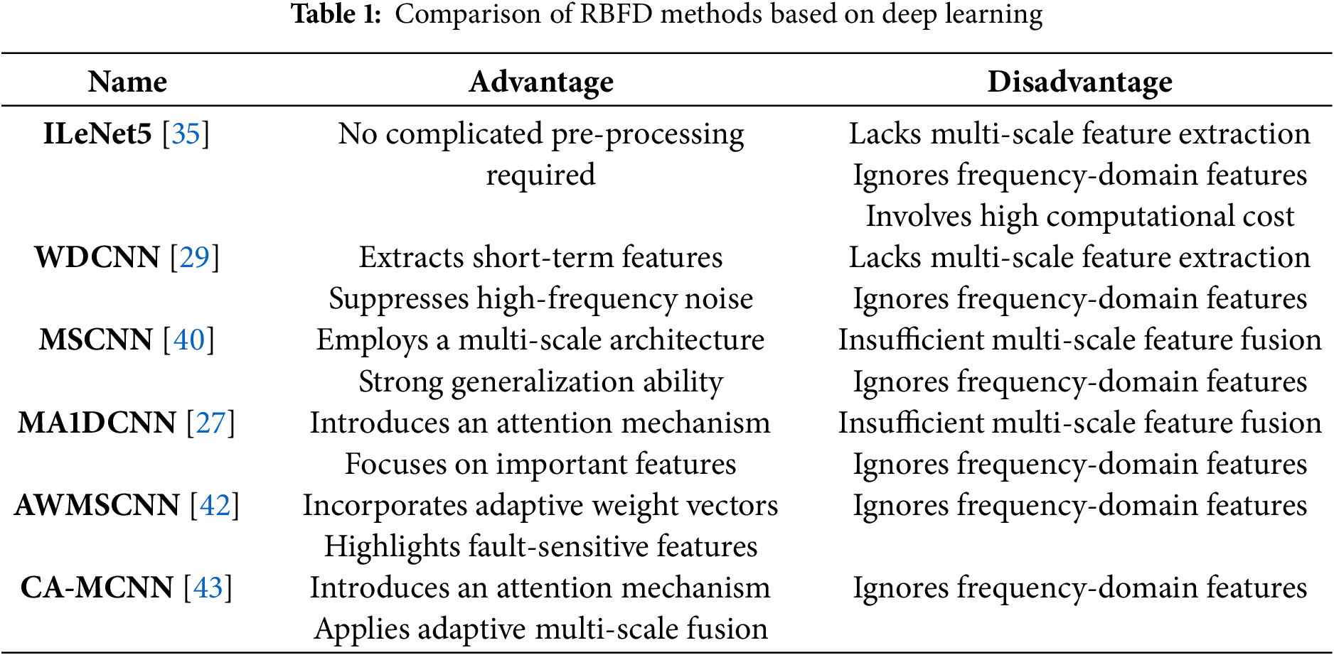
Multi-Scale CNN integrates convolutional layers with different kernel sizes to capture features at various temporal or frequency scales. This architecture has been widely applied in time-series classification and fault diagnosis tasks [39]. Reference [27] proposes a Multi-Scale One-Dimensional CNN with an attention mechanism (MA1DCNN), which embeds attention modules at different network depths to adaptively optimize feature mapping. Reference [40] proposes a Multi-Scale CNN (MSCNN), which enhances feature representation by processing vibration signals at different scales. Reference [41] proposes a Multi-Scale Cascade CNN (MC-CNN), which concatenates features extracted using convolutional kernels of various lengths to form composite representations for fault diagnosis. Reference [42] proposes an Adaptive Weighted Multi-Scale CNN (AWMSCNN), where convolutional layers with different kernel sizes are adaptively weighted and fused to extract rich and complementary features. Reference [43] proposes a Multi-Scale CNN with Channel Attention (CA-MCNN), which employs a 1D convolution-based parallel fusion mechanism to effectively capture and integrate complementary multi-scale information. The deep learning-based RBFD methods are shown in Table 1.

The multi-scale convolutional network employs convolutional kernels of varying scales, allowing the model to be trained simultaneously and thereby enhancing its adaptability. However, it has the following limitations in RBFD:

(1) Most multi-scale architectures rely on feature concatenation for fusion, which neglects the interactions between key features across different scales. This results in feature redundancy and inconsistency [44].

(2) Signal acquisition is often affected by factors like noise in real industrial environments, which increases the complexity and uncertainty of the signals. It is difficult to effectively represent fault characteristics by directly using time-domain signals.

The vibration signal generated by rolling bearings is non-stationary and nonlinear. Its frequency characteristics exhibit distinct peaks in the spectrum. Frequency-domain analysis can more efficiently extract fault-related frequency features and help identify the fault type. Commonly used frequency-domain analysis methods include wavelet transform (WT) and short-time Fourier transform (STFT). However, each of these methods has its limitations. WT requires selecting an appropriate basis function. STFT requires choosing a window function, and its time and frequency resolution cannot be optimized simultaneously. In contrast, the fast Fourier transform (FFT) has the advantages of fast processing speed, no need for preset parameters, and high frequency resolution [45]. However, the main drawback of FFT is that it computes over the entire period. This makes it difficult to distinguish between the stationary and transient components of the signal [46].

To address the above issues, this paper proposes an RBFD method based on MSFN. Meanwhile, to optimize frequency-domain feature extraction, a method is designed using multi-level and multi-size filters. MSFN simultaneously extracts both time-domain and frequency-domain features from the signal. By integrating the TDFT module with the convolution module, the model’s ability to represent non-stationary fault signals is significantly enhanced. Through multi-scale convolution and TDFT processing, the network selectively retains or suppresses frequency components, highlights key features, and strengthens critical information in the signal. Additionally, a cross-attention mechanism is introduced to fuse features across different scales, which effectively alleviates feature redundancy and improves the fault diagnosis performance. The main contributions of this paper are as follows:

(1) To address the issue that time-domain signals alone may not effectively represent fault characteristics, this paper proposes an RBFD method based on MSFN. It simultaneously extracts both time-domain and frequency-domain features, thereby significantly improving fault classification accuracy.

(2) A frequency-domain feature extraction method using multi-level, multi-size filters is designed. It effectively overcomes the limitations of FFT in distinguishing stationary and transient components by adaptively capturing both global and local frequency characteristics.

(3) A cross-attention mechanism is incorporated to enhance multi-scale feature fusion. It dynamically computes correlations between multi-scale features, adaptively selects key information, and reduces redundancy and conflicts in the fusion process.

(4) The proposed method is validated on the Ottawa [11] and CWRU [25] datasets. Experimental results show that MSFN achieves high diagnostic accuracy and strong generalization under variable noise and load conditions.

The rest of this paper is organized as follows. Section 2 provides an overview of MSFN. Section 3 explains the mathematical theory of TDFT and the frequency-domain feature extraction process. Section 4 presents the experimental process, results, and analysis. Finally, Section 5 concludes the paper.

2  Proposed Method

MSFN consists of four modules: (1) Feature screening: Preliminary screening is performed on the input fault signals. (2) Feature extraction: Multi-scale channels are constructed, and the time-frequency domain features of the signal are simultaneously extracted. (3) Feature fusion: A cross-attention mechanism is applied to fuse multi-scale feature information. (4) Fault classification: The integrated features are input into a classifier to determine the bearing fault category. The overall structure of the model is illustrated in Fig. 1.

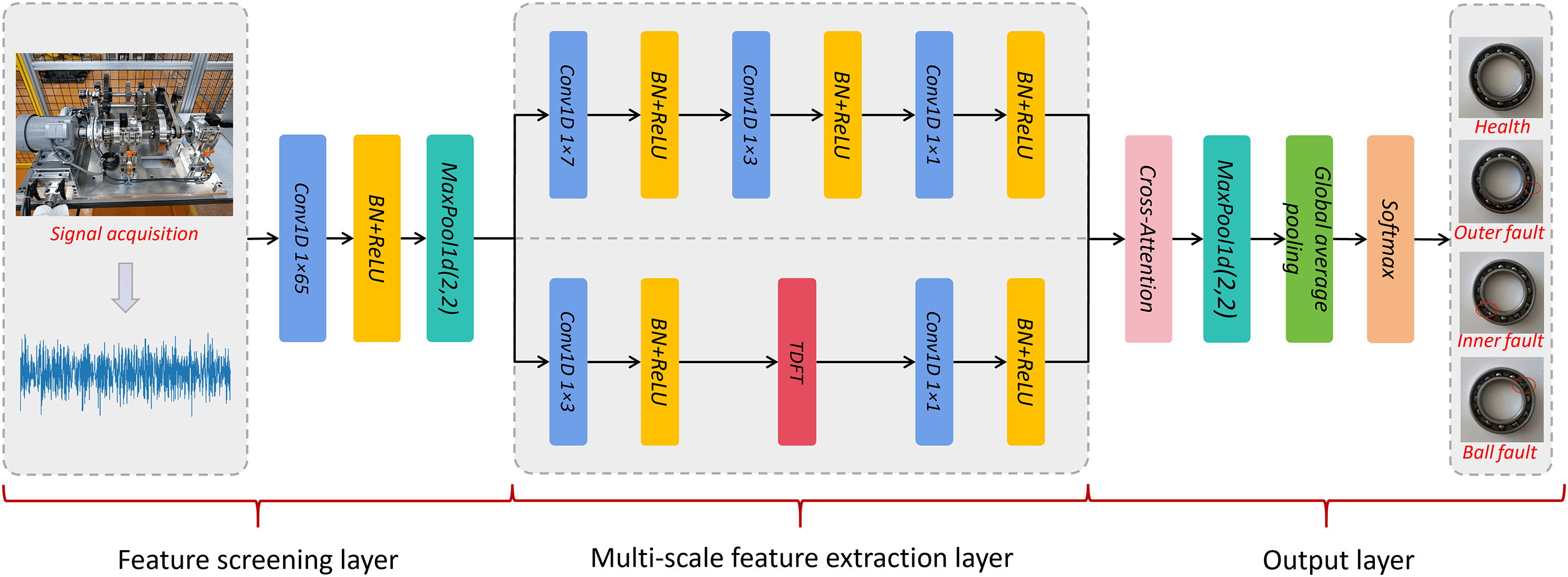
Figure 1: MSFN model

2.1 Feature Screening and Extraction

The feature screening module employs a 1 × 65 convolutional kernel to preliminarily process the input signal. Batch normalization and max-pooling are applied to reduce computational complexity. Finally, the ReLU activation function is used to accelerate the training.

In the feature extraction module, the preprocessed signal is divided into two parallel channels to extract features from both the time and frequency domains. A small convolutional kernel is employed in the time-domain channel to further extract time-domain features. Each convolutional operation is followed by batch normalization and the ReLU activation function. The ReLU activation is defined as:

ReLU(x)=max(0,x)(1)

where x is the network input. In the frequency-domain channel, the TDFT module extracts the signal envelope and performs frequency-domain filtering. The filtered signal is transformed back into the time domain via the Inverse Fast Fourier Transform (IFFT). This ensures consistency with the shape of the input signal.

2.2 Feature Fusion and Fault Classification

In the feature fusion module, feature information from the two channels is fused using a cross-attention mechanism. This mechanism enables interaction between different input sequences. It allows the model to focus on the most relevant content in the other sequence that is closely related to the current task. One input sequence generates the key K and value V, and another input sequence generates the Q in the cross-attention mechanism. The Q and K are used to calculate the similarity matrix through the dot product:

Score(Q,K)=QKTdk(2)

where dk is the dimension of the key vector, used to scale the dot product result to prevent the value from becoming excessively large. The SoftMax function is applied to convert the similarity matrix into a normalized attention weight matrix. This matrix represents the importance distribution across positions in the key-value sequence. Finally, the attention weight matrix is multiplied by the value matrix V to obtain the weighted feature representation:

Attention(Q,K,V)=Softmax(QKTdk)V(3)

The output of the cross-attention mechanism is a weighted sum of the value vectors. It is the information dynamically aggregated from the key-value sequence based on the query sequence. The principle of the cross-attention mechanism is illustrated in Fig. 2.

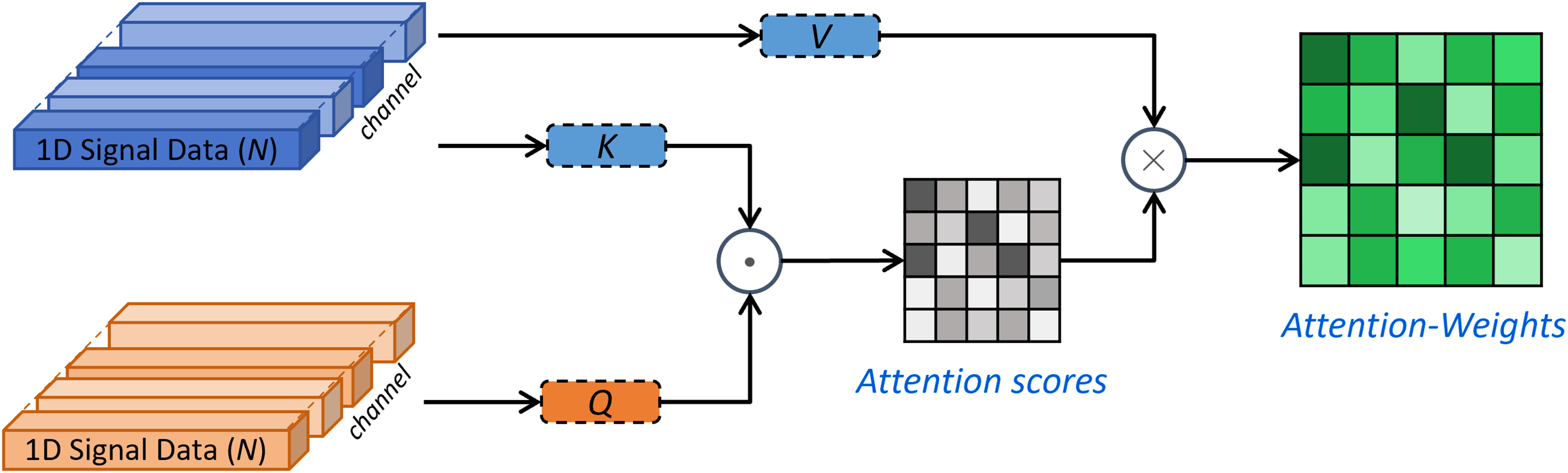
Figure 2: Cross-attention mechanism

In the fault classification module, the fused features are processed using global average pooling. This operation reduces the number of parameters, retains global contextual information, and enhances the model’s generalization capability. Finally, a SoftMax classifier is employed to produce the final fault diagnosis results.

3  Time-Division Fourier Transform

In the TDFT module, filters of different sizes are generated according to the length of the input signal. The time-domain signal is segmented into fixed-size windows corresponding to the filter sizes. Batch normalization is applied to each window to reduce batch-to-batch variability. The normalized signal is then subjected to the Hilbert transform to extract envelope features. Subsequently, the FFT is applied to convert the signal from the time-domain to the frequency-domain. Frequency-domain filtering is performed using complex-valued weights to extract features from multiple frequency bands. The filtered frequency-domain signal is transformed back to the time-domain using IFFT, ensuring that the output shape matches the input. The extracted features are temporarily stored in a feature list for subsequent processing. The overall process is illustrated in Fig. 3.

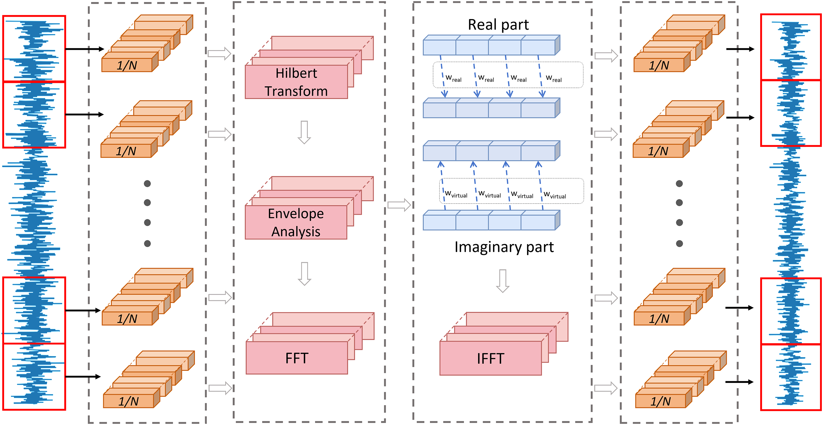
Figure 3: Single-layer frequency-domain feature extraction

In the multi-level feature extraction process, the signal is re-divided into larger windows, and the aforementioned steps are repeated. The features extracted at each level correspond to frequency-domain characteristics captured by filters of varying sizes. These features collectively form a set of multi-scale representations. After extracting features at all levels, a set of learnable weights is applied to perform weighted fusion across different scales. The overall framework is illustrated in Fig. 4. The multi-scale feature fusion can dynamically balance the contributions of features from different frequency bands.

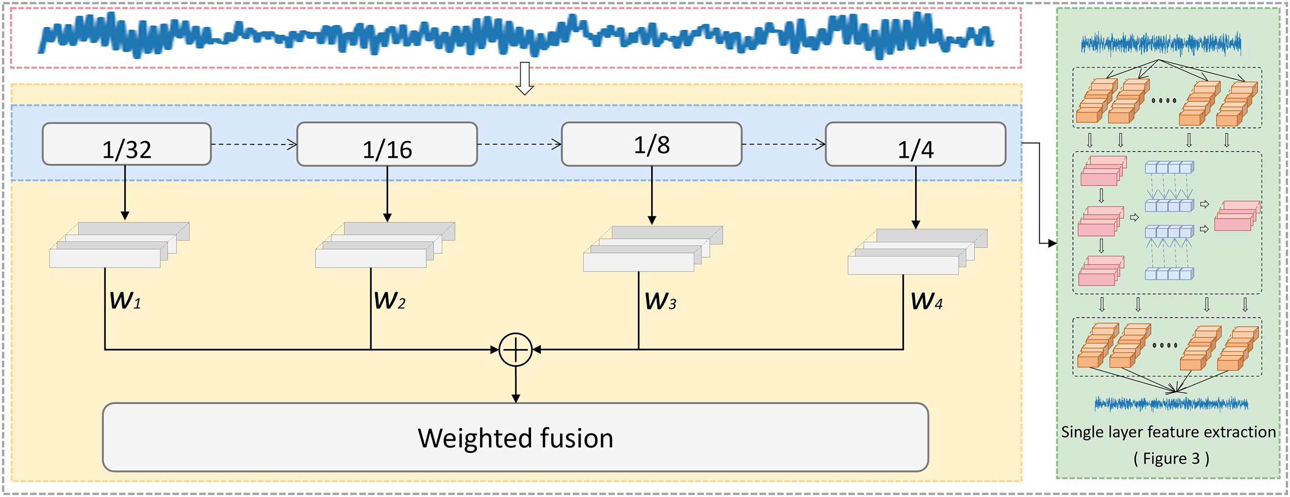
Figure 4: Multi-layer frequency-domain feature extraction

3.1 Signal Segmentation

The input signal is denoted as t∈RB×C×N, where B, C, and N are the batch size, number of channels, and signal length. Filters are generated based on the input signal length N and a set of filter ratios rk. The length Lk of each filter is computed as follows:

Lk=max(8,⌈N⋅rk⌉)(4)

where k is the index of the filter. A learnable weight wk is assigned to each filter.

The input signal is divided into fixed-size windows based on the filter length, where each window has a length of Lk, and the signal is segmented into P=⌈N/Lk⌉ segments. Each segment of the signal is processed through batch normalization to reduce batch-to-batch variation:

xp(t)=xp(t)−μσ2+ϵ⋅γ+β,p=1,2,…,P(5)

where p is the index of each fragment. μ and σ2 are the mean and variance of the input data. ϵ is a small constant used to prevent division by zero errors. γ and β are learnable scaling and translation parameters.

3.2 Hilbert Transform and Envelope Analysis

The Hilbert transform provide the envelope and instantaneous frequency of a signal. This helps reveal more latent features, which aids in fault identification and classification during the diagnostic process. For a signal xp(t), its Hilbert transform is defined as x^p(t):

x^p(t)=H[xp(t)]=1π∫−∞∞xp(τ)t−τdτ(6)

where H[xp(t)] is the Hilbert transform. τ is the integral variable, representing the value of the signal at different time points. The Hilbert transform yields the imaginary part of the signal x^p(t), which is orthogonal to the original signal xp(t).

The original signal xp(t) and its Hilbert transform x^p(t) are combined into a complex-valued signal to obtain the analytic signal zp(t):

zp(t)=xp(t)+jx^p(t)(7)

where j is the imaginary unit. The real part of the analytical signal is still the original signal xp(t), and the imaginary part provides the instantaneous phase information of the signal.

Envelope analysis is a technique used to extract the low-frequency components of a signal by filtering out its high-frequency components. The envelope ap(t) of the signal is obtained by analyzing the amplitude of the signal zp(t):

ap(t)=|zp(t)|=xp(t)2+x^p(t)2(8)

3.3 Frequency-Domain Filtering

FFT is an algorithm for efficiently computing the discrete Fourier transform (DFT) and its inverse transform. By exploiting the periodicity and symmetry of the rotation factors to reduce the computational complexity of DFT from O(N2) to O(N{log}N). The envelope signal ap(t) is transformed into the frequency-domain using FFT, resulting in the frequency-domain signal x^p(t):

x^p(f)=FFT[ap(t)](9)

where complex weights wk are used to implement frequency-domain filtering. The filtered frequency-domain signal is then restored to the time domain using the IFFT, reconstructing its original shape, as follows:

y(t)=∑p=1PIFFT[x^p(f)⋅wk](10)

3.4 Multi-Level Feature Fusion

To further capture frequency-domain features at different time scales, the signal is re-divided into larger windows, and the signal at each scale undergoes a single-layer feature extraction step:

ym(t)=∑p=1PIFFT[x^p(f)⋅wk],m=1,2,…,M(11)

where m is the index of different scales, and M is the total number of scales. The features from all scales are dynamically balanced through weighted fusion:

y(t)=∑m=1Mλm⋅ym(t)(12)

where λk is the learnable fusion weight for different scales, which adaptively adjusts the contribution of features from different scales according to task requirements.

The final feature integrates multi-scale and multi-frequency band information. In TDFT, the signal’s frequency components are selectively retained or suppressed to highlight key features and reduce noise interference.

4  Experimental Validations

4.1 Experimental Settings

To evaluate the fault diagnosis performance of the proposed method, experiments are conducted on the Case Western Reserve University (CWRU) and University of Ottawa (Ottawa) rolling bearing datasets. The one-dimensional vibration signal is divided into training, validation, and test datasets through overlapping sampling. The experimental settings are batch size 64, epoch is 50, and learning rate is 0.001. PyTorch 2.3.1 is used as the deep learning framework. The hardware environment is configured with an Intel(R) Core(TM) i7-13700KF @ 2.50 GHz CPU, an RTX 3090 (24 GB) GPU, and 64 GB of memory. The software environment consists of Windows 11, Python 3.12.4, and PyTorch 2.3.1 with CUDA 12.6.

The experiment selected accuracy, precision, F1 score, specificity, AUC, and model average inference time as evaluation indicators for the model’s fault diagnosis performance, along with an analysis of model complexity. These indicators are crucial for a comprehensive evaluation of diagnostic models, particularly under industrial constraints.

•   Accuracy: The overall proportion of correctly classified samples.

•   Precision: The proportion of correctly predicted positive cases among all predicted positives.

•   Recall: The proportion of actual positive cases that are correctly predicted by the model.

•   F1-score: The harmonic mean of precision and recall, reflecting the balance between them.

•   Specificity: The ability of the model to correctly identify negative cases.

•   AUC (Area Under the Curve): The area under the ROC curve, representing the trade-off between true positive and false positive rates. A higher AUC indicates stronger discriminative capability across thresholds.

•   Average Inference Time: The average time taken by the model to predict a single input sample.

4.2 Data Description

4.2.1 CWRU Dataset

The dataset is configured with four load conditions: 0, 1, 2, and 3 HP. The sampling frequencies include 12 and 48 kHz, and this paper uses the data from the drive-end bearing with a sampling frequency of 12 kHz. The dataset consists of four states: normal, inner race fault, outer race fault, and ball fault. For each fault type, there are three fault diameters: 0.1778, 0.3556, and 0.5334 mm. The data collected under the four load conditions (0, 1, 2, and 3 HP) are organized into four datasets: Datasets ①, ②, ③, and ④. Each dataset contains 10 states (Normal, B007, B014, B021, IR007, IR014, IR021, OR007, OR014, OR021). Each dataset corresponding to a load condition includes 10,000 samples, totaling 40,000 samples across all four datasets. To prevent overfitting due to insufficient sample size, overlapping sampling is employed to increase the number of samples. The formula for the overlapping sampling operation is as follows:

G=N−N1D+1(13)

where G is the number of samples in a single class. N is the length of the one-dimensional signal. N1 is the length of the signal segment, and D is the step size. The signal segment length is 1024, and each dataset is divided into training, validation, and test sets in a 7:2:1 ratio.

4.2.2 Ottawa Dataset

The dataset was collected using the SpectraQuest Mechanical Fault Simulator (MFS-PK5M). It contains vibration and rotational speed data of rolling bearings with various fault types and simulates multiple operating conditions, including acceleration, deceleration, acceleration followed by deceleration, and deceleration followed by acceleration. Each operating condition includes five health states: healthy, inner race fault, outer race fault, ball fault, and compound fault. Based on different operating conditions, Datasets ①, ②, ③, and ④ are created, with each dataset containing 5000 samples. Each signal segment has a length of 1024, and the datasets are split into training, validation, and test sets in a ratio of 7:2:1.

4.3 Optimization Analysis

In addition to the model architecture, the performance of fault diagnosis is also affected by the training process. In this experiment, the Adam optimizer is adopted. The Adam optimizer has adaptive learning rates and momentum update characteristics. It employs exponentially weighted moving averages to estimate the momentum and second moment of the gradients. The basic form of parameter update given the objective function L(θ) is formulated as follows:

θt=θt−1−η∇θL(θt−1)(14)

where η is the learning rate. ∇θL(θt−1) is the gradient at the t iteration.

To further optimize the training process, the CWRU dataset under a single load condition was utilized, with Datasets ①, ②, and ③ selected as experimental samples. The proposed model was evaluated by comparing optimization algorithms, including Adam, SGD with momentum, RMSProp, AdaGrad, and AdaDelta. The experimental results are shown in Fig. 5.

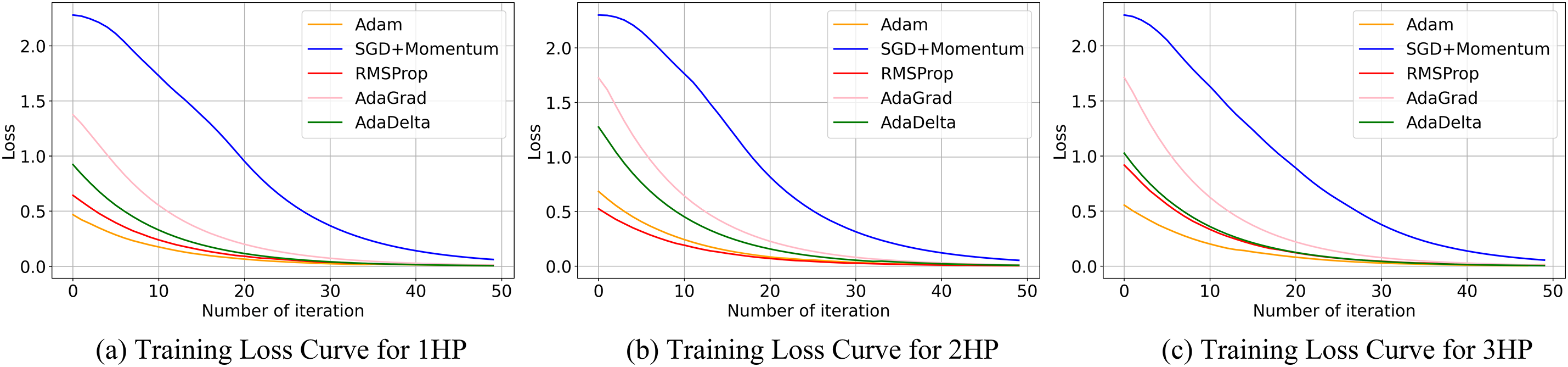
Figure 5: Comparison of convergence speed of optimization algorithms

As shown in the figure, when using the Adam optimizer on Datasets ① and ③, the model converges significantly faster than with other optimization algorithms.

4.4 Noise Interference Scenario Simulation Experiment

Rolling bearing signal data is often obscured by complex noise in real industrial environments, increasing the complexity of the signal data. To verify the noise robustness of the proposed model, Gaussian white noise with varying intensities is added to the experimental data, simulating noisy interference scenarios that better represent real-world operating conditions. In this experiment, the Signal-to-Noise Ratio (SNR) is used to measure noise intensity, expressed in decibels (dB):

SNRdB=10log10(PsignalPnoise)(15)

where SNRdB, Psignal, and Pnoise are the SNR, signal amplitude, and noise amplitude. After adding noise, the original features are obscured by the noise. As the SNR decreases, the extent to which the features are masked by the noise becomes more severe.

This experiment uses the CWRU dataset and selects dataset ④ as the experimental sample. Gaussian white noise with SNRs ranging from 0 to 10 dB is added to simulate noise interference. The performance of the proposed model is compared with three baseline models: ILeNet5 [35], WDCNN [29], and MSCNN [40]. Additionally, to assess the effectiveness of the TDFT module and the advantage of using cross-attention for feature fusion, two ablation models are included for comparison. The first, MSFN_FFT, employs a standard FFT to extract frequency-domain features. The second, MSFN_NCA, uses simple feature concatenation to integrate multi-scale features. The fault diagnosis results of each model under different SNR levels are presented in Fig. 6 and Table 2.

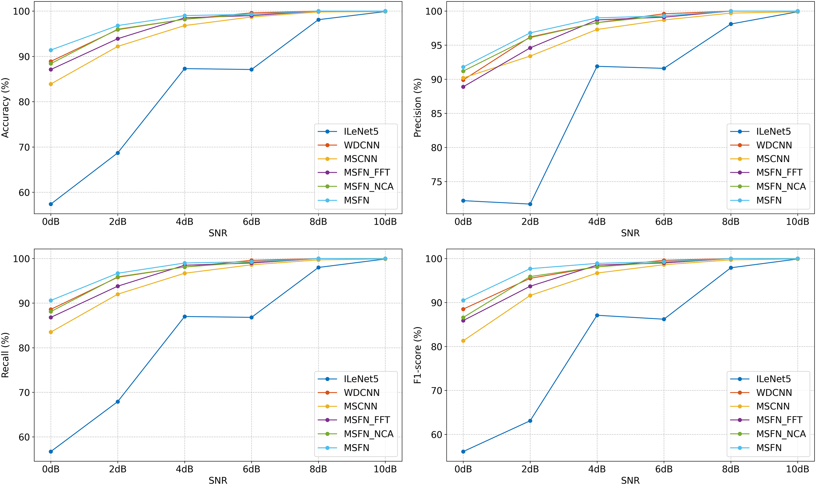
Figure 6: Comparison of diagnostic effects under different SNR (CWRU)

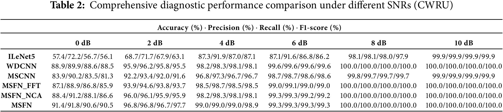
As shown in the figure, most models exhibit higher diagnostic accuracy under low noise conditions. However, under high noise levels, the performance of models such as ILeNet5, WDCNN, and MSCNN degrades significantly. For instance, ILeNet5 achieves only 57.4% accuracy at 0 dB and 68.7% at 2 dB, indicating that shallow or purely time-domain convolutional architectures struggle to preserve fault-related features in the presence of strong noise interference signals. In contrast, deeper models such as WDCNN and MSCNN benefit from their hierarchical feature extraction capabilities and demonstrate stronger robustness, especially at SNRs above 4 dB. For instance, WDCNN achieves an average accuracy of 97.1%, maintaining over 95% accuracy even at 2 dB.

Although the MSFN_FFT model extracts frequency-domain features from the signal, its performance remains suboptimal under strong noise conditions. This suggests that simple FFT-based approaches are limited in their ability to capture fault-relevant frequency features in complex, noisy signals. The MSFN_NCA uses simple feature concatenation to integrate multi-scale features and achieves an average accuracy of 96.98%. The MSFN model further improves upon this, attaining an average accuracy of 97.75%. Compared to ILeNet5, WDCNN, MSCNN, MSFN_FFT, and MSFN_NCA, the improvements are 14.67%, 0.65%, 2.53%, 1.33%, and 0.77%. This comparison with the MSFN_NCA model highlights that the cross-attention mechanism enhances the network’s ability to emphasize informative features while effectively suppressing noise interference.

Overall, although all models exhibit good performance at higher SNRs, the MSFN model maintains consistently high accuracy across all noise levels, demonstrating superior stability and adaptability in noisy environments. To further assess the model’s feature extraction and fault classification capabilities under high noise conditions, confusion matrices are constructed. These matrices represent the model’s classification performance at SNR levels of 0 and 2 dB. The visualized results are shown in Fig. 7.

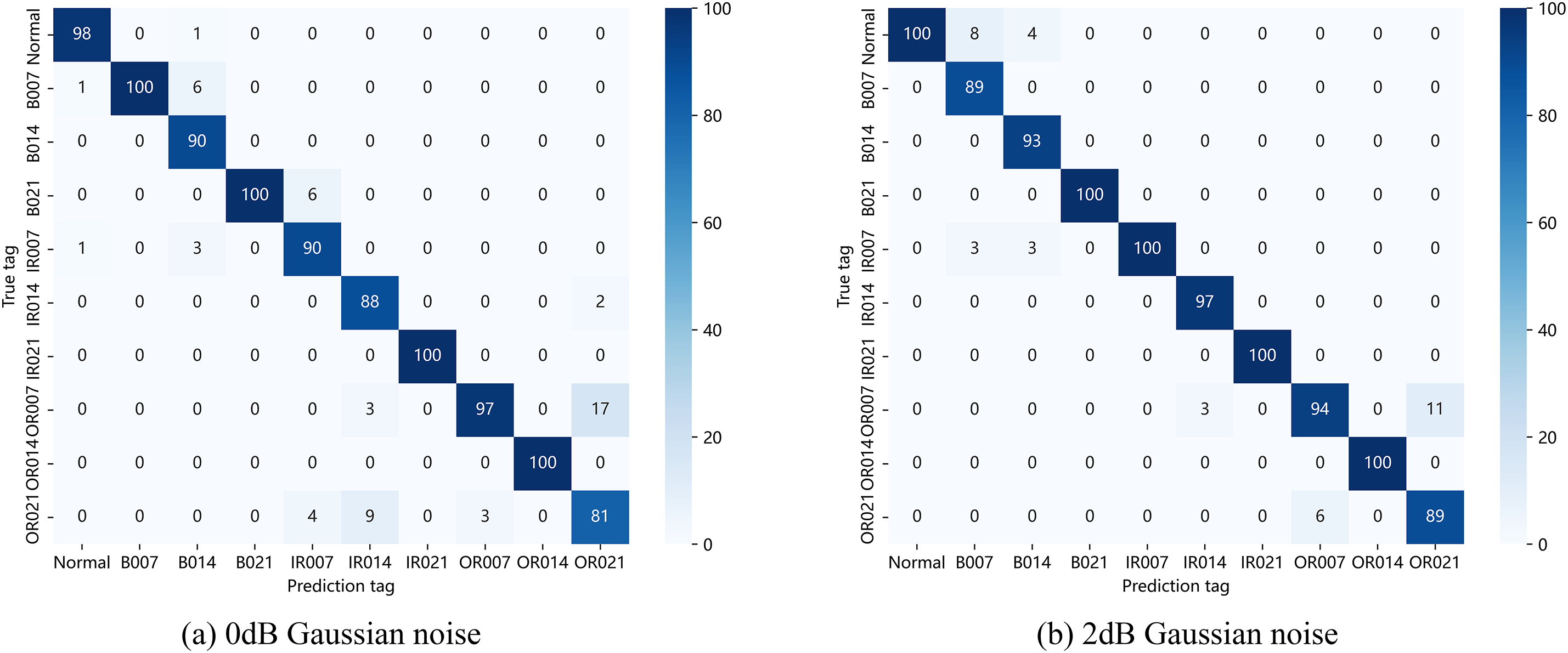
Figure 7: Confusion matrix at 0 and 2 dB SNR

As shown in the figure, the proposed method can maintain a high accuracy even at SNRs of 0 and 2 dB, indicating that the method exhibits notable resistance to noise. To further assess its feature extraction capability, t-SNE was employed for dimensionality reduction and visualization of features extracted at different layers under an SNR of 4 dB. The visualization results are shown in Fig. 8.

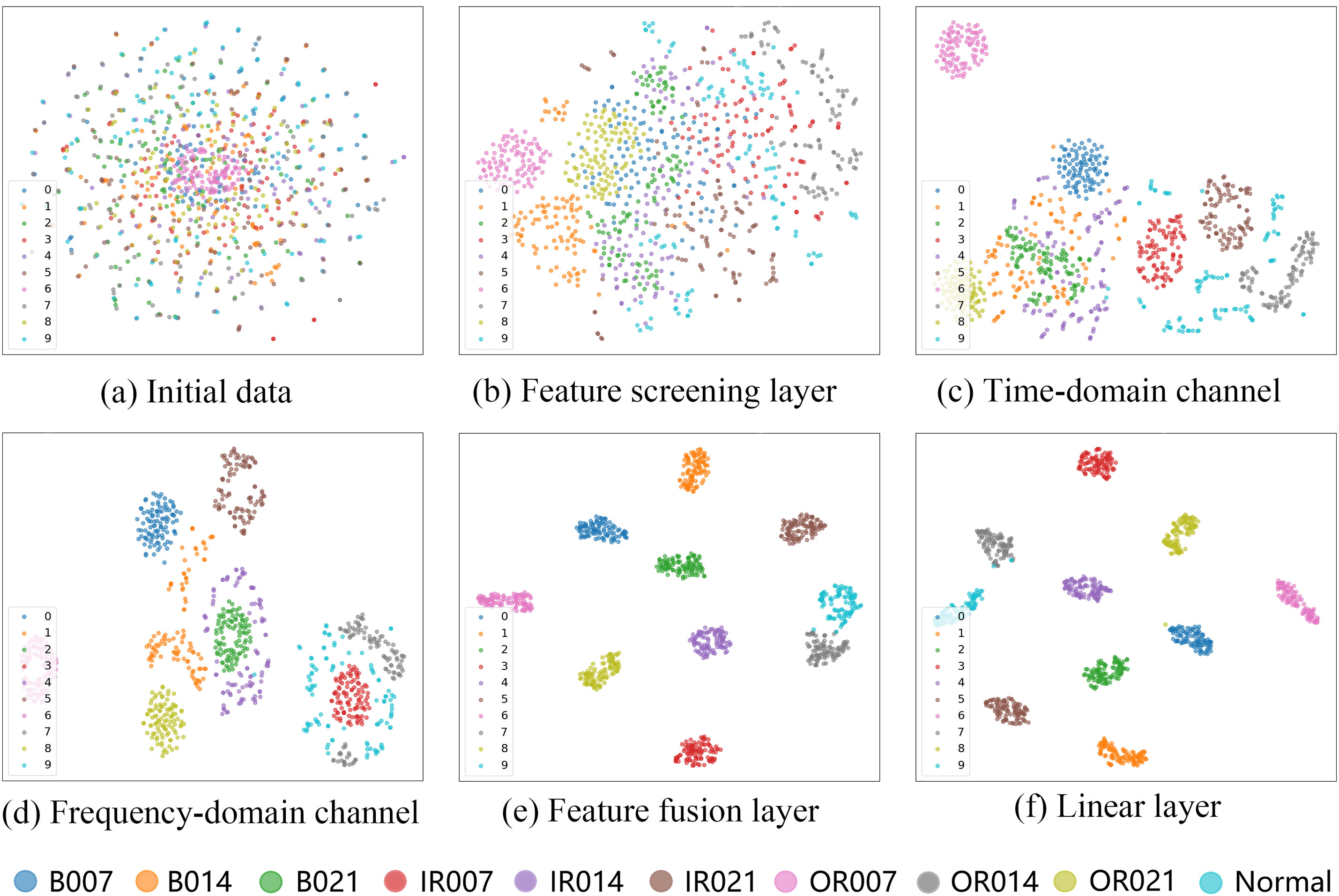
Figure 8: t-SNE dimensionality reduction visualization

Fig. 8a shows the results of dimensionality reduction and visualization applied directly to the raw data. Data from different categories overlap and blend. Fig. 8b shows the results after initial feature selection using large convolution kernels. Although different types of data still exhibit significant overlap, there are signs of clustering. Fig. 8c and d shows the results after the data passes through the time-domain feature channel and the frequency-domain feature channel. It can be observed that some fault types have already been clustered. Fig. 8e shows the result after the time-frequencydomain feature information is fused using the cross-attention mechanism. The data is almost entirely divided into 10 categories, with a clear clustering effect for each sample. Fig. 8f shows the result after passing through the fully connected layer, where the clustering effect is more pronounced. By comparing Fig. 8b and e, it can be seen that the proposed method has significant feature extraction ability.

The specificity of each model under different SNR conditions is illustrated in Fig. 9. The six axes represent SNR levels ranging from 0 to 10 dB, while the plotted curves correspond to different models. It can be observed that specificity generally increases with higher SNR levels, indicating that noise significantly impairs the models’ ability to correctly identify negative samples. Notably, the MSFN and WDCNN models maintain consistently high specificity even at lower SNRs. In contrast, ILeNet5 exhibits a more compressed curve, reflecting a weaker capability to suppress false positives under noisy conditions. These results further demonstrate the robustness of MSFN against noise interference.

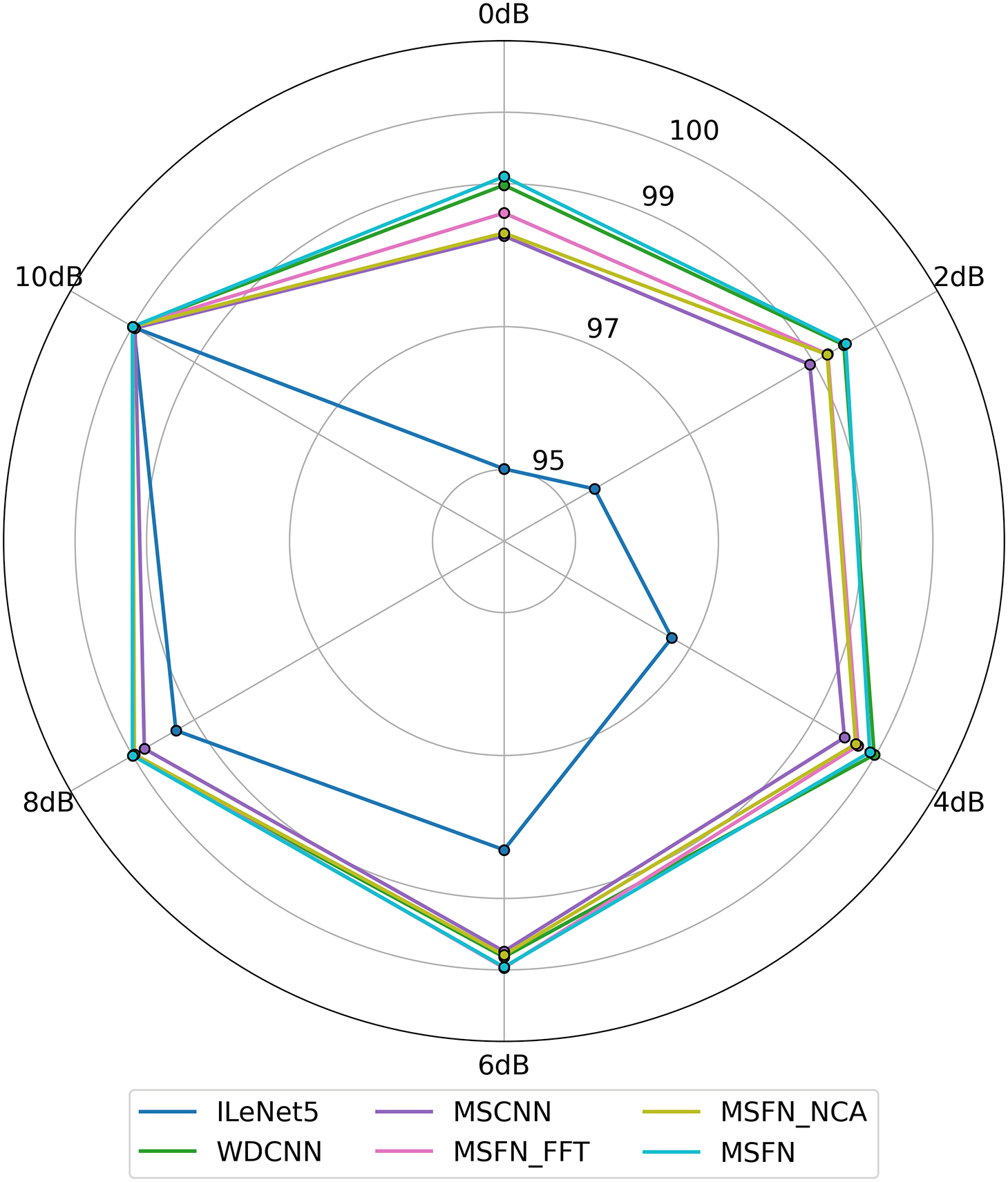
Figure 9: Radar chart of specificity for different models under varying noise levels (SNR)

Fig. 10 shows the ROC curves of the MSFN, ILeNet5, MSCNN, and WDCNN models at 0 dB SNR along with their corresponding AUC values. It can be seen that the ROC curves of MSFN and WDCNN are close to the top-left corner, with AUC values of 0.9993 and 0.9972, indicating excellent discriminative capability. MSCNN also performs well, achieving an AUC of 0.9838. In contrast, ILeNet5 shows a relatively lower AUC of 0.8359, reflecting its limited generalization ability in noisy environments.

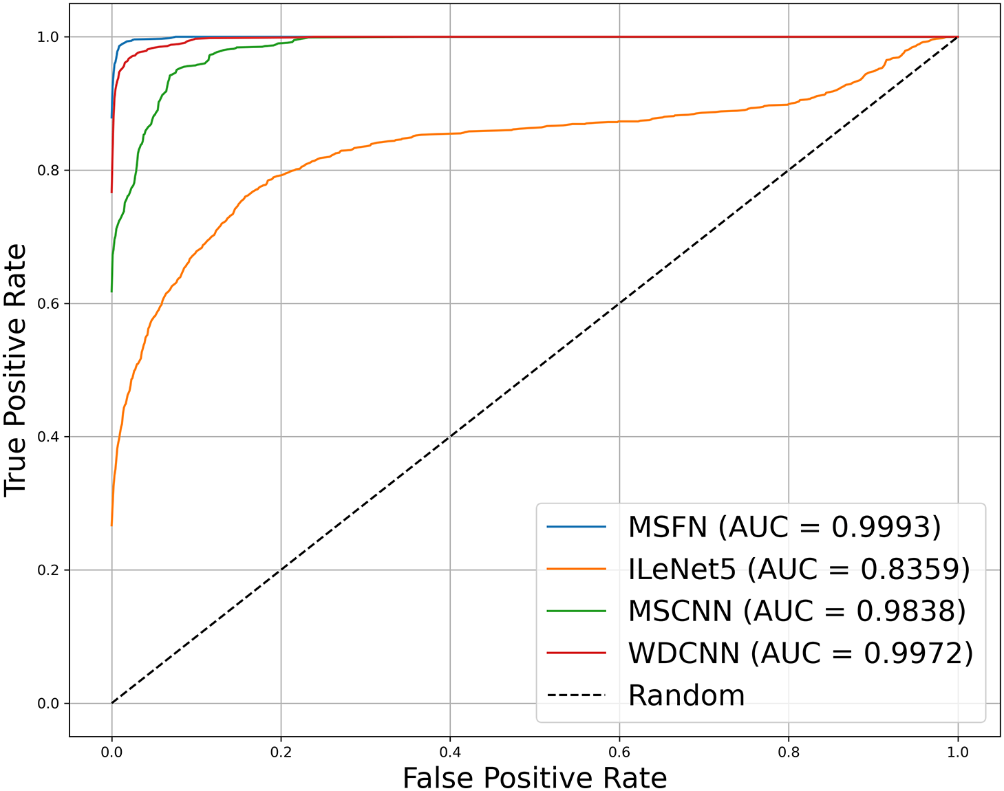
Figure 10: Comparison of ROC curves and AUC values under noise interference (SNR = 0 dB)

4.5 Variable Load Scenario Simulation Experiment

The load conditions of rolling bearings often change in actual industrial environments. This requires diagnostic methods to have a strong generalization ability. To evaluate the generalization capability of the proposed method, fault diagnosis experiments were conducted under varying load conditions. This experiment uses the CWRU dataset and employs datasets ①, ②, and ③ as training samples, with fault diagnosis performed on the remaining datasets. For example, ‘①→②’ means using dataset ① as the training set to train the model and dataset ② as the test set to perform fault diagnosis. The training parameters are set the same as those in the noise interference experiment. The diagnostic results of each method under variable load conditions are shown in the Fig. 11 and Table 3.

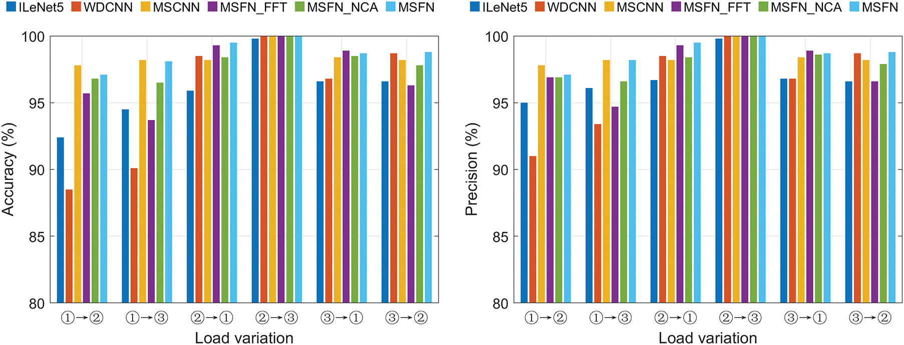
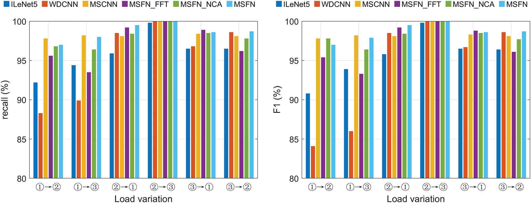
Figure 11: Comparison of diagnostic effects under variable load

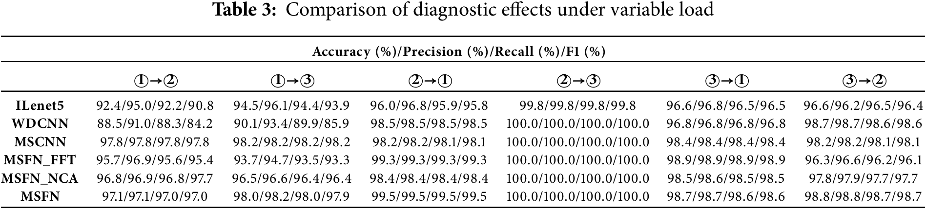
As shown in the figure, ILeNet5 and WDCNN exhibit low fault diagnosis accuracy under variable load conditions, indicating that these models have certain limitations in generalization under such conditions. Specifically, under variable load tasks, the performance of these models fluctuates significantly, which may be influenced by substantial changes in the input data. In contrast, MSCNN and the proposed model can still maintain high accuracy under variable load conditions, achieving 98.47% and 98.68%. This result demonstrates that the multi-scale model improves adaptability to varying inputs while enhancing expressive ability, thereby showing better generalization performance, particularly in complex load change scenarios. Moreover, the proposed method shows an improvement in accuracy compared to other models, with increases of 2.70%, 3.25%, 0.21%, 1.36%, and 0.68%. These results suggest that the proposed method retains a certain level of generalization capability under variable load conditions, indicating its adaptability to load variations.

4.6 Model Universality Experiment

To verify the universality of the proposed method on different datasets, experiments are conducted using the Ottawa dataset. Dataset ② is selected as the experimental sample. Gaussian white noise with an SNR ranging from 0 to 10 dB is added to simulate various noises during the signal acquisition process. The experimental results are compared with the ILeNet5, WDCNN, MSCNN, MSFN_FFT, and MSFN_NCA models, as shown in Table 4.

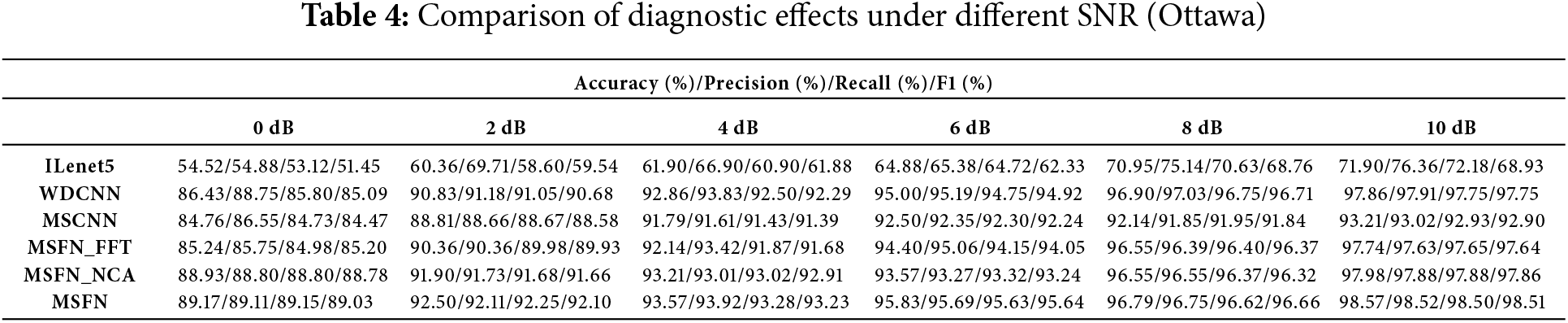
The accuracy of all models generally decreases in this experiment. This may be attributed to the precision of the data acquisition device and the environment in which the data is collected. As shown in the figure, the accuracy of the proposed model remains high on this dataset, with an average accuracy of 94.41%. Even under 0dB noisy signals, it can maintain an accuracy of nearly 90%, indicating that the proposed method exhibits a certain degree of universality.

4.7 Model Complexity Analysis

Although the proposed model achieves high diagnostic performance by integrating multi-scale time-frequency domain feature extraction and cross-attention fusion, it introduces certain computational burdens, mainly attributed to two components:

(1) TDFT module, which involves repeated envelope extraction using Hilbert transforms and frequency-domain filtering via FFT and IFFT. The complexity is approximately:

𝒪(M⋅B⋅C⋅Nlog⁡N)(16)

where M is the number of filter scales, B is Batchsize, C is channels, and N is the input signal length.

(2) The CrossAttention module, operating on time-domain and frequency-domain features, performs full attention with complexity:

𝒪(B⋅2⋅S2⋅dk)(17)

where 2 refers to processing features from two branches (time domain/frequency domain), S is the sequence length, and dk is the key dimension. It should be noted that the attention mechanism introduces a computational bottleneck due to its quadratic growth with respect to sequence length.

Although the total parameter count remains moderate, the model is computationally expensive, especially in real-time scenarios with long signals. Future work will focus on exploring lightweight approximations to reduce computational costs.

Table 5 shows the average inference time of each model under different noise conditions. Overall, traditional models such as ILeNet5, WDCNN, and MSCNN exhibit high inference speeds, with an average time of under 1 millisecond. This makes them suitable for deployment on edge devices with stringent real-time requirements. While the MSFN models have outstanding performance in accuracy and robustness, their inference overhead is slightly higher, with an average inference time ranging from 1 to 4 milliseconds.

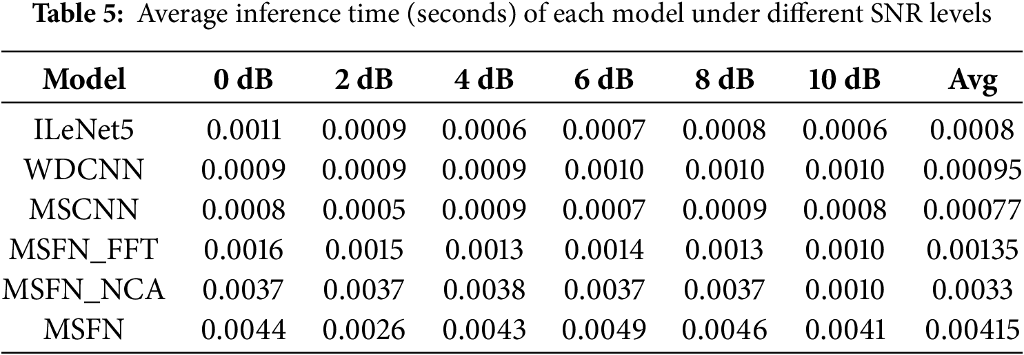
It is worth noting that the inference time of the MSFN models is relatively high, primarily due to the inclusion of attention mechanisms and feature reconstruction modules. These components add computational complexity. Therefore, in practical applications, a trade-off must be made between accuracy and efficiency, depending on device performance and real-time requirements.

5  Conclusion

This paper proposes an RBFD method based on a multi-scale time-frequency domain fusion network. The approach extracts time-domain and frequency-domain features from vibration signals and employs a cross-attention mechanism to enhance multi-scale feature fusion. Under complex noise and variable load conditions, the method improves both diagnostic accuracy and robustness. Additionally, a frequency-domain feature extraction method with multi-level, multi-size filters is designed, overcoming the FFT’s limitation in distinguishing between stationary and transient signal components.

Despite the promising performance, the proposed model still exhibits certain limitations. The incorporation of the TDFT and cross-attention mechanisms introduces considerable computational overhead, which may hinder real-time deployment. Moreover, the model’s performance is sensitive to the selection of hyperparameters in the TDFT module, such as window length and filter ratios. This may affect its stability and generalizability across different operating scenarios. Future work will focus on the following directions.

(1) Model compression and pruning can reduce computational complexity and memory consumption. This makes the model more suitable for deployment in real-time or embedded industrial environments.

(2) Adaptive TDFT mechanisms, such as learning-based windowing strategies or dynamic filter generation, to improve robustness and reduce reliance on manual parameter tuning.

(3) Hardware acceleration strategies, including deployment on edge devices with GPU/FPGA support or integration with efficient inference engines like TensorRT or ONNX Runtime.

(4) Exploring domain adaptation or transfer learning frameworks to enhance cross-domain generalization, especially when the model is applied to other types of rotating machinery or operating environments not seen during training.

Acknowledgement: The authors would like to express sincere gratitude to all the anonymous reviewers and the editorial team for their valuable comments and suggestions.

Funding Statement: This work is fully supported by the Frontier Exploration Projects of Longmen Laboratory (No. LMQYTSKT034); Key Research and Development and Promotion of Special (Science and Technology) Project of Henan Province, China (No. 252102210158)

Author Contributions: Ronghua Wang, as the first author, was responsible for the conception and design of the MSFN model and was the main contributor to the paper. Shibao Sun was responsible for the collection and processing of the bearing fault dataset. Pengcheng Zhao was responsible for the validity verification of the MSFN model and the analysis of experimental results. Xianglan Yang reviewed the manuscript and proposed suggestions for control experiments. Xingjia Wei and Changyang Hu assisted in collecting and collating relevant literature, participated in the discussion of experimental results, and revised the paper. All authors reviewed the results and approved the final version of the manuscript.

Availability of Data and Materials: Data supporting the findings of this study may be obtained from the corresponding authors upon reasonable request.

Ethics Approval: Not applicable.

Conflicts of Interest: The authors declare no conflicts of interest to report regarding the present study.

References

1. Zhao M, Zhong S, Fu X, Tang B, Pecht M. Deep residual shrinkage networks for fault diagnosis. IEEE Trans Ind Inform. 2020;16(7):4681–90. doi:10.1109/tii.2019.2943898. [Google Scholar] [CrossRef]

2. Wang Y, Yang M, Zhang Y, Xu Z, Huang J, Fang X. A bearing fault diagnosis model based on deformable atrous convolution and squeeze-and-excitation aggregation. IEEE Trans Instrum Meas. 2021;70:3524410. doi:10.1109/tim.2021.3109721. [Google Scholar] [CrossRef]

3. Zhang X, Zhao B, Lin Y. Machine learning based bearing fault diagnosis using the case western reserve university data: a review. IEEE Access. 2021;9:155598–608. doi:10.1109/access.2021.3128669. [Google Scholar] [CrossRef]

4. Liu R, Yang B, Zio E, Chen X. Artificial intelligence for fault diagnosis of rotating machinery: a review. Mech Syst Signal Process. 2018;108(7):33–47. doi:10.1016/j.ymssp.2018.02.016. [Google Scholar] [CrossRef]

5. An D, Liu Z, Shao M, Li X, Hu R, Shi M, et al. Fault diagnosis of bearing-rotor system based on infrared thermography: reSPP with multi-scaled training method. Meas Sci Technol. 2023;34(12):125030. doi:10.1088/1361-6501/acf2b1. [Google Scholar] [CrossRef]

6. An Y, Zhang K, Liu Q, Chai Y, Huang X. Rolling bearing fault diagnosis method base on periodic sparse attention and LSTM. IEEE Sens J. 2022;22(12):12044–53. doi:10.1109/jsen.2022.3173446. [Google Scholar] [CrossRef]

7. Zheng H, Yang Y, Yin J, Li Y, Wang R, Xu M. Deep domain generalization combining a priori diagnosis knowledge toward cross-domain fault diagnosis of rolling bearing. IEEE Trans Instrum Meas. 2021;70:3501311. doi:10.1109/tim.2020.3016068. [Google Scholar] [CrossRef]

8. Habbouche H, Amirat Y, Benkedjouh T, Benbouzid M. Bearing fault event-triggered diagnosis using a variational mode decomposition-based machine learning approach. IEEE Trans Energy Convers. 2022;37(1):466–74. doi:10.1109/tec.2021.3085909. [Google Scholar] [CrossRef]

9. Van M, Kang HJ. Bearing defect classification based on individual wavelet local fisher discriminant analysis with particle swarm optimization. IEEE Trans Ind Inform. 2016;12(1):124–35. doi:10.1109/tii.2015.2500098. [Google Scholar] [CrossRef]

10. Zhang S, Zhang S, Wang B, Habetler TG. Deep learning algorithms for bearing fault diagnostics—a comprehensive review. IEEE Access. 2020;8:29857–81. doi:10.1109/access.2020.2972859. [Google Scholar] [CrossRef]

11. Pu H, Zhang K, An Y. Restricted sparse networks for rolling bearing fault diagnosis. IEEE Trans Ind Inform. 2023;19(11):11139–49. doi:10.1109/tii.2023.3243929. [Google Scholar] [CrossRef]

12. Peng Z, Song X, Song S, Stojanovic V. Spatiotemporal fault estimation for switched nonlinear reaction-diffusion systems via adaptive iterative learning. Int J Adapt Control Signal Process. 2024;38(10):3473–83. doi:10.1002/acs.3885. [Google Scholar] [CrossRef]

13. Barai V, Ramteke SM, Dhanalkotwar V, Nagmote Y, Shende S, Deshmukh D. Bearing fault diagnosis using signal processing and machine learning techniques: a review. IOP Conf Ser Mat Sci Eng. 2022;1259(1):012034. doi:10.1088/1757-899x/1259/1/012034. [Google Scholar] [CrossRef]

14. Zhang N, Wu L, Yang J, Guan Y. Naive bayes bearing fault diagnosis based on enhanced independence of data. Sensors. 2018;18(2):463. doi:10.3390/s18020463. [Google Scholar] [PubMed] [CrossRef]

15. Lin H, Zhang X, Li H. Bearing fault diagnosis based on BP neural network. IOP Conf Ser Earth Environ Sci. 2018;208:012092. doi:10.1088/1755-1315/208/1/012092. [Google Scholar] [CrossRef]

16. Cheng Y, Wang Z, Zhang W, Huang G. Particle swarm optimization algorithm to solve the deconvolution problem for rolling element bearing fault diagnosis. ISA Trans. 2019;90:244–67. doi:10.1016/j.isatra.2019.01.012. [Google Scholar] [PubMed] [CrossRef]

17. Ben Ali J, Fnaiech N, Saidi L, Chebel-Morello B, Fnaiech F. Application of empirical mode decomposition and artificial neural network for automatic bearing fault diagnosis based on vibration signals. Appl Acoust. 2015;89:16–27. doi:10.1016/j.apacoust.2014.08.016. [Google Scholar] [CrossRef]

18. Xiao M, Liao Y, Bartos P, Filip M, Geng G, Jiang Z. Fault diagnosis of rolling bearing based on back propagation neural network optimized by cuckoo search algorithm. Multimed Tools Appl. 2021;81(2):1567–87. doi:10.1007/s11042-021-11556-x. [Google Scholar] [CrossRef]

19. Shao X, Wang L, Kim CS, Ra I. Fault diagnosis of bearing based on convolutional neural network using multi-domain features. KSII Transact Inter Inform Syst (TIIS). 2021;15(5):1610–29. doi:10.3837/tiis.2021.05.002. [Google Scholar] [CrossRef]

20. Wang S, Lian G, Cheng C, Chen H. A novel method of rolling bearings fault diagnosis based on singular spectrum decomposition and optimized stochastic configuration network. Neurocomputing. 2024;574(2):127278. doi:10.1016/j.neucom.2024.127278. [Google Scholar] [CrossRef]

21. Hoang DT, Kang HJ. A survey on Deep Learning based bearing fault diagnosis. Neurocomputing. 2019;335(7):327–35. doi:10.1016/j.neucom.2018.06.078. [Google Scholar] [CrossRef]

22. Dong Y, Jiang H, Liu Y, Yi Z. Global wavelet-integrated residual frequency attention regularized network for hypersonic flight vehicle fault diagnosis with imbalanced data. Eng Appl Artif Intell. 2024;132:107968. doi:10.1016/j.engappai.2024.107968. [Google Scholar] [CrossRef]

23. Zeng T, Jiang H, Liu Y, Bai Y. AHWCN: an interpretable attention-guided hierarchical wavelet convolutional network for rotating machinery intelligent fault diagnosis. Expert Syst Appl. 2025;272:126815. doi:10.1016/j.eswa.2025.126815. [Google Scholar] [CrossRef]

24. Li Z, Liu F, Yang W, Peng S, Zhou J. A survey of convolutional neural networks: analysis, applications, and prospects. IEEE Trans Neural Netw Learn Syst. 2022;33(12):6999–7019. doi:10.1109/tnnls.2021.3084827. [Google Scholar] [PubMed] [CrossRef]

25. Jiang Y, Shi Z, Tang C, Sun J, Zheng L, Qiu Z, et al. Cross-conditions fault diagnosis of rolling bearings based on dual domain adversarial network. IEEE Trans Instrum Meas. 2023;72:3533915. doi:10.1109/tim.2023.3322485. [Google Scholar] [CrossRef]

26. Peng D, Liu Z, Wang H, Qin Y, Jia L. A novel deeper one-dimensional CNN with residual learning for fault diagnosis of wheelset bearings in high-speed trains. IEEE Access. 2019;7(1):10278–93. doi:10.1109/access.2018.2888842. [Google Scholar] [CrossRef]

27. Wang H, Liu Z, Peng D, Qin Y. Understanding and learning discriminant features based on multiattention 1DCNN for wheelset bearing fault diagnosis. IEEE Trans Ind Inform. 2020;16(9):5735–45. doi:10.1109/tii.2019.2955540. [Google Scholar] [CrossRef]

28. Junior RFR, Areias IAdS, dos S, Campos MM, Teixeira CE, da Silva LEB, et al. Fault detection and diagnosis in electric motors using 1D convolutional neural networks with multi-channel vibration signals. Measurement. 2022;190(8):110759. doi:10.1016/j.measurement.2022.110759. [Google Scholar] [CrossRef]

29. Zhang W, Peng G, Li C, Chen Y, Zhang Z. A new deep learning model for fault diagnosis with good anti-noise and domain adaptation ability on raw vibration signals. Sensors. 2017;17(2):425. doi:10.3390/s17020425. [Google Scholar] [PubMed] [CrossRef]

30. Wen L, Li X, Gao L, Zhang Y. A new convolutional neural network-based data-driven fault diagnosis method. IEEE Trans Ind Electron. 2018;65(7):5990–8. doi:10.1109/tie.2017.2774777. [Google Scholar] [CrossRef]

31. Xia M, Li T, Xu L, Liu L, de Silva CW. Fault diagnosis for rotating machinery using multiple sensors and convolutional neural networks. IEEE/ASME Trans Mechatron. 2018;23(1):101–10. doi:10.1109/tmech.2017.2728371. [Google Scholar] [CrossRef]

32. Husari F, Seshadrinath J. Stator turn fault diagnosis and severity assessment in converter-fed induction motor using flat diagnosis structure based on deep learning approach. IEEE J Emerg Sel Top Power Electron. 2023;11(6):5649–57. doi:10.1109/jestpe.2022.3184754. [Google Scholar] [CrossRef]

33. Liu K, Li Z, He W, Peng J, Wang X, Wang Y. A fault diagnosis method based on wavelet denoising and 2DCNN under background noise. In: 2023 IEEE 12th Data Driven Control and Learning Systems Conference (DDCLS); 2023 May 12–14; Xiangtan, China. p. 530–5. [Google Scholar]

34. He W, Mao J, Liu L, Li Z, Yang M, Wang Y. A muti-stage selection filter based on wavelet packet and 2DCNN for fault diagnosis of rotating machinery. In: 2023 42nd Chinese Control Conference (CCC); 2023 Jul 24–26; Tianjin, China. p. 4951–5. [Google Scholar]

35. Wan L, Chen Y, Li H, Li C. Rolling-element bearing fault diagnosis using improved LeNet-5 network. Sensors. 2020;20(6):1693. doi:10.3390/s20061693. [Google Scholar] [PubMed] [CrossRef]

36. Sun Y, Tao H, Stojanovic V. Autoregressive data generation method based on wavelet packet transform and cascaded stochastic quantization for bearing fault diagnosis under unbalanced samples. Eng Appl Artif Intell. 2024;138(4):109402. doi:10.1016/j.engappai.2024.109402. [Google Scholar] [CrossRef]

37. Dong Y, Jiang H, Wu Z, Yang Q, Liu Y. Digital twin-assisted multiscale residual-self-attention feature fusion network for hypersonic flight vehicle fault diagnosis. Reliab Eng Syst Saf. 2023;235:109253. doi:10.1016/j.ress.2023.109253. [Google Scholar] [CrossRef]

38. Wang X, Jiang H, Mu M, Dong Y. A dynamic collaborative adversarial domain adaptation network for unsupervised rotating machinery fault diagnosis. Reliab Eng Syst Saf. 2025;255:110662. doi:10.1016/j.ress.2024.110662. [Google Scholar] [CrossRef]

39. Chen W, Shi K. Multi-scale attention convolutional neural network for time series classification. Neural Netw. 2021;136(2):126–40. doi:10.1016/j.neunet.2021.01.001. [Google Scholar] [PubMed] [CrossRef]

40. Jiang G, He H, Yan J, Xie P. Multiscale convolutional neural networks for fault diagnosis of wind turbine gearbox. IEEE Trans Ind Electron. 2019;66(4):3196–207. doi:10.1109/tie.2018.2844805. [Google Scholar] [CrossRef]

41. Huang W, Cheng J, Yang Y, Guo G. An improved deep convolutional neural network with multi-scale information for bearing fault diagnosis. Neurocomputing. 2019;359(3):77–92. doi:10.1016/j.neucom.2019.05.052. [Google Scholar] [CrossRef]

42. Qiao H, Wang T, Wang P, Zhang L, Xu M. An adaptive weighted multiscale convolutional neural network for rotating machinery fault diagnosis under variable operating conditions. IEEE Access. 2019;7:118954–64. doi:10.1109/access.2019.2936625. [Google Scholar] [CrossRef]

43. Huang YJ, Liao AH, Hu DY, Shi W, Zheng SB. Multi-scale convolutional network with channel attention mechanism for rolling bearing fault diagnosis. Measurement. 2022;203(3):111935. doi:10.1016/j.measurement.2022.111935. [Google Scholar] [CrossRef]

44. Xue L, Lei C, Jiao M, Shi J, Li J. Rolling Bearing fault diagnosis method based on self-calibrated coordinate attention mechanism and multi-scale convolutional neural network under small samples. IEEE Sens J. 2023;23(9):10206–14. doi:10.1109/jsen.2023.3260208. [Google Scholar] [CrossRef]

45. Zhang M, Yin J, Chen W. Rolling bearing fault diagnosis based on time-frequency feature extraction and IBA-SVM. IEEE Access. 2022;10(5):85641–54. doi:10.1109/access.2022.3198701. [Google Scholar] [CrossRef]

46. Anwarsha A, Narendiranath Babu T. Recent advancements of signal processing and artificial intelligence in the fault detection of rolling element bearings: a review. J Vibroeng. 2022;24(6):1027–1055. doi:10.21595/jve.2022.22366.. [Google Scholar] [CrossRef]