Developing Fault Prognosis and Detection Modes for Main Hoisting Motor in Gantry Crane Based on t-SNE

1  Introduction

In response to the rising demand for international trade, container terminals in various regions have also established newly built remote operator container yards [1]. This remote control container system is also known as an automated container system. As shown in Fig. 1, these shipyards do not station personnel next to the equipment to minimize potential hazards and allow the crank system to run at peak efficiency [2]. However, this makes remote monitoring of the component crucial to the crank system because the absence of an on-site operator cannot hear and feel the noises and vibrations in the control room as before.

Figure 1: (a) Remote controlled bridge crane; (b) Remote operator

Machine Health Index. With the continuous advancement of manufacturing technology, the complexity of modern systems has increased to follow the ever-rising demand for production efficiency, operational stability, and personnel safety. Predicting the remaining lifespan of a machine is then essential in intelligent diagnosis as it would help improve production efficiency and reduce maintenance costs [3]. Predictive Health Management (PHM) is increasingly important within the machinery field. It is typically used to monitor rotating parts such as bearings or gears. The PHM aims to change the traditional “failure before repair” strategy. The PHM insists on creating a “prediction for prevention” strategy. The difference between diagnostics and prognostics is when the action takes place. Diagnostics is the process of identifying the root cause of a problem after it has occurred. It is a passive maintenance method of waiting for the damage to happen. Prognostics is a proactive maintenance method that evaluates the current health of the machine and predicts where failures are likely to occur [4]. Artificial neural networks are used on collected sensor data to extract characteristic features and classify the machine’s state [5].

Non-Stationary Signal. The vibration signal observed from the main crane motor in this study is classified as a non-stationary signal. While operating the machine, the frequency recorded from the motor continuously changes during the loading and unloading of containers. According to the literature, condition monitoring of rotating machinery under variable speed conditions is a challenging task. As such, this topic is a very active research area. Specifically, the unique non-stationary signals coming from the vibrations generated by these machines [6]. This complex non-stationary signal can then be decomposed into multiple stationary signals based on the local characteristic time scale of the signal [7]. The sensor tools monitor its status and present the results in time and frequency domains [8]. Frequency domain methods in the literature provide a way to detect faults. The Fast Fourier Transform (FFT) is a commonly used technique that can convert the signal from the time domain to the frequency domain to generate a spectral signal analysis. The FFT is based on the assumption of signal periodicity. This would, by definition, not be suitable for non-stationary signals. Time-frequency analysis of non-stationary signals is a better approach [9].

Fault Detection. Recently, many industrial machines have had bearing damage from operating variable frequency motors and motor failure caused by bearing currents [10]. Motor abnormalities can occur in different ways, such as electrical or mechanical failure, rotor failure, stator failure, bearing failure, eccentricity failure, etc. Various signal processing methods are utilized to obtain different fault characteristics, which must be done without disassembly to reduce maintenance costs and time [11]. Machine learning for feature extraction has achieved considerable results. The features studied by the neural network are based on the pre-processed vibration signal. The feature average and root mean square (RMS) values are key features. The model is trained to look for these features to predict failure and prevent damage [12]. The sensor used to measure vibrational movement, called an accelerometer, converts the mechanical movement experienced into an electronic signal. The exact type or model of sensor used depends on the specifications needed, such as frequency range, sensitivity, and operating limitations. No matter which type of accelerometer is used, attaching it closer to the source will yield a higher accuracy and sensitivity. Tahmasbi et al. measured large motors during acceleration and coast-down processes, and employed frequency trend analysis to identify the causes of motor faults [13]. To ensure the status of the sensing node of the wireless sensor network, Duche and Sarwade proposed a failure detection approach for the fault-tolerant [14]. For their proposed Round Trip Delay (RTD) method, several sensor network topologies can be selected to evaluate the faulty sensor on a minimal energy basis.

Machine Learning. As pointed out in [5], large data sets are generally complex and difficult to interpret clearly. It is necessary to employ additional methods to enhance the accuracy of further analyzing the large data set [5,15]. This study focuses on the feasibility of using the primary motor dataset in machine learning, where fault classification involves many complex characteristics that affect the accuracy of classification recognition [16]. Vibration analysis is widely used for fault detection and diagnosis in measuring mechanical and machine tool rotation. Machine learning methods for detecting tool fault features include Principal Component Analysis (PCA) for data dimensionality reduction and Support Vector Machines (SVM) for feature classification [17]. Recently, many scholars have proposed methods to classify features in data for motor fault analysis and diagnostics to clarify feature identification. Kumar and Abdulkareem et al. use the NN model and the feature extraction method to identify different motor failures (e.g., ball bearing fault, load imbalance, and so on) [18,19]. Gao et al. first proposed a Multi-source Domain Information Fusion Network (MDIFN), which leverages adversarial transfer learning along with various other methods to improve fault diagnosis accuracy under different operating conditions of the rotation machine. Subsequently, they developed a Domain Feature Disentanglement Network (DFDN), enabling the model to handle unseen working conditions through fault feature separation and related techniques, even without target-domain samples [20,21]. From these methods, the use of t-SNE has been selected for this purpose [22]. The approach of this method is data fusion to reduce dimensionality and display a 2-dimensional representation of the data. The results are then compared to the actual data set for verification [23]. When mechanisms or motors experience faults or abnormalities, accelerometers can trigger signal acquisition, usually collected from signal analysis throughout the operation. The t-SNE can deal with high-dimensional data by superiorly visualizing it. For fault characteristics, t-SNE demonstrates the best dimensionality reduction and clustering effect [24].

The reviewed research works delight us with the great insight into the techniques of diagnosing machines. However, little research has been done on the faulty detection of the operational main hoisting motor in the gantry crane system. Thus, this study focuses on Kaohsiung Port, which operated its new fully automated shipping terminal in 2023. This new terminal utilizes both unmanned equipment and remote-controlled equipment. Inside the new terminal are a total of five 18-m deep ship docks. Each ship dock has independent remote-controlled Bridge Gantry cranes (GC), Automated Rail-Mounted Gantry cranes (ARMG), and Container Stackers. This study aims to establish one such system to monitor and analyze the vibratory signals of the system and determine the location of faults or damages. The goal is to help maintenance personnel determine the issue faster and precisely, and based on our work, can monitor remotely in the near future.

2  Experimental Setup and Signal Pre-Processing

Fig. 2 shows the flowchart of this research. In the beginning, we installed an acceleration meter to measure the vibration of the crane’s operation. Second, we used signal processing to convert the time-domain vibration data to frequency-domain data, and the band calculation was also used for subsequent feature-band selection. The above two sections will be explained in Section 2. Third, we used the t-SNE and t-SNE result rating methods to verify that the selected band could identify different machines’ normal or abnormal conditions, as explained in Section 3. Finally, an NN model was trained with the feasible band chosen to classify the different machine operation conditions, shown in Section 4.

Figure 2: The flowchart of this research

As shown in Fig. 3, the schematic shows the power module of the crank system, and the layout includes the AC inverter motor, the reduction gearbox, the wire rope drum, and the measurement locations. Fig. 4a denotes the specifications of the sensors and data acquisition module (DAQ with AD7606 chip), and Fig. 4b indicates their locations on the motor housing. The MEMS-type accelerometer (ADXL 1005 chip) and the peripheral circuit are connected to a dual-channel DAQ before connecting to the on-site laptop.

Figure 3: Power module of the crank system

Figure 4: Vibratory signal measuring experiment setup; (a) Specifications of accelerometer and data acquisition module; (b) Installation of accelerometer and data acquisition module

Preliminary analysis of abnormal events is focused on the continuous operation of the main hoist motor and each complete movement of the gantry crane and claw for lifting and lowering motion. The lifting motion of the container stops when it reaches the upper limit. The trolley then moves toward the desired position overhead of the desired location on the ground or vessel. Next, the crane claw descends until the container reaches the target, as shown in Fig. 5. The accelerometers record all the variations of vibratory signals throughout the process. To compromise the bandwidth of ADXL 1005, the sampling rate of our ADC is tuned down to 12 Ks/s, which means 12,000 samples per second. Fig. 6 presents the time signals for more than 55 s for one complete normal and abnormal status movement. Thus, the bottom of Fig. 6 depicts the spectrogram for the frequency variations with time. From observation, operation under normal conditions presents clear frequency peaks, even with the non-stationary signals. However, the spectrogram spreads at high amplitudes in a wide frequency band in the event of an abnormal operation. The task for the next step is to determine how we can retrieve the features of the operational conditions.

Figure 5: One complete movement of the gantry crank system includes lifting, horizontal moving, and lowering

Figure 6: The signals of one complete movement of the gantry crank system; (a) Normal state; (b) Abnormal state

We propose the selection of critical frequency bands to reduce the size dimension of signals with time and frequency parameters. From the preliminary analysis, the excited bandwidth spreads between low frequency 3 kHz, and we, therefore, divide the results of Fast Fourier Transform (FFT) to 100 Hz per unit bandwidth from 1 to 3 kHz. Thus, we have a total of 30 sets of average (AVG) amplitude for each set without overlapping.

For further interpretation, the vibratory amplitudes are measured during the action of the main crane motor. Each bar denotes one band for 100 Hz in size, and the magnitude is the average result of all amplitudes corresponding to frequencies in this bandwidth. Fig. 7 depicts the motor normal and abnormal AVG amplitudes and the 30 sets of the frequency band range from 1 to 3000 Hz. The differences are well distinguishable, and the same conclusions can also be observed in the case of motor cooling fan normal and abnormal in Fig. 8. We can see the difference between a normal fan and an abnormal one, which is not as significant as that of the motor. That’s because the motor might be a little damaged when we acquired the fan data. Hence, if we see the figure of the motor as abnormal and the fan as normal, we can observe that they share similar features. For easier judgment in subsequent analyses, we will use motor normal data as the normal sample, as everything was fully repaired during the motor normal data measurement.

Figure 7: Comparison of frequency bands for motor normal and abnormal

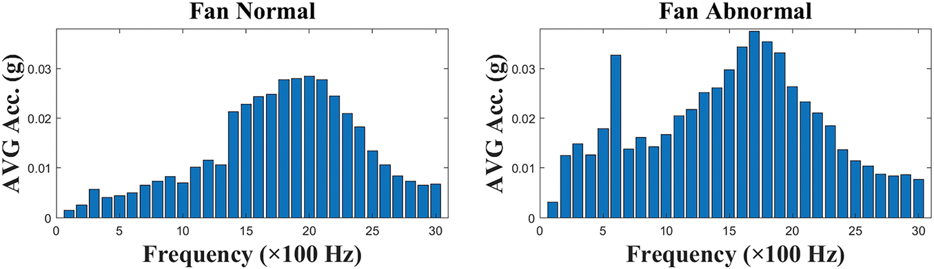
Figure 8: Comparison of frequency bands for fan normal and abnormal

For convenience sake, the results in Figs. 7 and 8 are computed in ratio, in which the abnormal AVG amplitude (including fan abnormal, fan normal, and motor abnormal) is divided by the normal AVG amplitude (motor normal) for each bandwidth. Fig. 9 shows the ratios of these three conditions, between 1 and 3000 Hz. We can see the ratios then considerably change between 900 and 2200 Hz. For instance, the ratios of 1100~1200, 1500, and 1800~2200 Hz bands both increase by over 5 times or even more. The significant variances of the vibration amplitudes can indicate the feature of the abnormal state. In this phase, we will first select the aforementioned bands as the base for the subsequent failure detection model. Although we have already selected some features, depending on the performance of the detection model or subsequent analysis, we may come back and retrieve additional bands or discard some as input features.

Figure 9: The ratio between the band of motor normal and 3 different abnormal conditions

In this section, we have concluded that selecting critical frequency bands can help observe the working states of motor motion. Although the information can alert the maintenance engineers at the remote site, more details of the failure components are still unrevealed within the massive crank system. In the next section, more acquired signals for specific failure events are classified based on our methodology.

3  Feature Visualization and Extraction with t-SNE Algorithm

In this section, we retrieved the maintenance log for analysis to further explore the specific abnormal components. We have aligned the time frame of vibratory signals with events, including fan abnormal (fan ABNL), fan repaired (fan NL), motor abnormal (motor ABNL), and normal states (NL). All ratios of the frequency bands are computed and depicted in Fig. 10. The denominators of the ratios are the AVG amplitudes of the motor in normal condition, and the numerators are the AVG amplitudes of the different conditions. The horizontal axis is the frequency band, and the vertical axis is the ratio of abnormal to normal AVG amplitudes for each band. The actual conditions for events were more complicated than we had thought, but it was a real situation in the field. In the top plot of Fig. 10, a technician detected the abnormal fan, but the bearing of the motor failure was not observed. Thus, the second plot of Fig. 10 shows insignificance with the top plot, between 1200 and 2000 Hz, even though the technician repaired the fan. The bottom plot of Fig. 10 presents the motor’s abnormal condition versus the normal state. To conclude the findings of the frequency band, the frequency band reveals more information for individual abnormal components, but it is unstructured. Therefore, we need a classification tool to identify and extract specific features from unstructured data. Here, we propose a method using t-Distributed Stochastic Neighbor Embedding (t-SNE) and a novel t-SNE rating method to search the feature automatically. The details will be elaborated upon in a later section.

Figure 10: Comparison of the three states of the fan and motor to the normal condition of the whole crank system

3.1 The Concept of t-SNE

The t-SNE, t-Distributed Stochastic Neighbor Embedding, is one of the statistical methods for visualizing high-dimensional data in lower-dimensional spaces. The high-dimensional data implies complex datasets, i.e., nonlinearity, like those that most serve as inputs in machine learning. In many applications, t-SNE is adopted to classify the data with limited information and can provide an efficient index of feature extraction for the following supervised learning.

Unlike the PCA, Principal Components Analysis, based on Euclid distance that works for linear data, t-SNE adopts the concept of preserving the similarity of data for dealing with both linear and nonlinear cases. Matten and Hinton proposed the joint probabilities of pairs of data points in the high-dimensional space rather than their sole distances [25]. The first step is the Stochastic Neighbor Embedding, which will convert Euclidean distances between data points in the high-dimensional space into conditional probabilities, p(j|i), that represent similarities. For instance, the conditional probability of two data points, xi and xj i ≠ j, is relatively high if these two data points are nearby and, on the contrary, the value of p(j|i) is low, referring to Eq. (1).

pj|i=exp⁡(−‖xi−xj‖2/2σi2)∑k≠iexp⁡(−‖xi−xk‖2/2σi2)(1)

The standard deviation, σi, is determined based on the density of nearby data points. However, how far the surrounding points shall be included can be defined by users in the named parameter “perplexity” in MATLAB or Python. The similarity, p(j|i), is in proportion to the probability density of Gaussian distribution centered at xi with zero mean, μ, and σi, denoted in Eq. (2). Since the t-SNE focuses on pairwise similarities, if there are n data points, for this xi, there are n * 1 numbers of density value mapped on the x-axis of the specific Gaussian plot for xi.

Y(x;μ,σi)=1σ2πexp⁡(−(x−μ)22σi2)(2)

Before we continue the t-SNE approach’s computation process, the original SNE’s inevitable issue can be addressed. The “crowding problem” is interpreted as, although the area of the high-dimensional space is available to accommodate moderately distant neighbors, the lower-dimensional space cannot preserve the pairwise similarities in the high-dimensional space, which will cause contradictions between data points. That is one of the crucial issues for nonlinear dimensionality reduction techniques. The t-SNE replaced the normal distribution initially utilized in lower-dimensional space with the student’s t-distribution, hereafter t-distribution, with one degree of freedom to alleviate the issue of the crowding problem. The t-distribution has heavier tails that allow the data points with moderate distance in the high-dimensional space to be classified as moderately dissimilar clusters in the lower-dimensional space. By comparing the normal distribution with the rapidly decaying boundaries, the t-distribution allows a more significant distance between similar and dissimilar clusters for distinguishing.

Then, the second step is to compute the similar conditional probability for the low-dimensional counterparts yi and yj of the high-dimensional data points xi and xj, referring to Eq. (3). If the data points yi and yj model correctly for the similarity between low-dimensional and high-dimensional data points, the conditional probabilities p(j|i) and qij shall be equal. The Kullback-Leibler divergence, hereafter KL, is adopted to measure the faithfulness between p(j|i) and qij, presented in Eq. (4). The summation of KL over all data points will be minimized by using gradient descent, denoted in Eq. (5).

qij=(1+‖yi−yj‖2)−1∑k≠j(1+‖yi−yj‖2)−1(3)

C=∑iKL(Pi||Qi)=∑i∑jpi|jlog⁡pj|iqj|i(4)

δCδyi=4∑i(pi|j−qi|j)(yi−yj)(5)

3.2 The Confusion of Visualization

The topic in this paragraph is deciding which frequency bands shall be included for computing in t-SNE. Intuitively, we shall pick the most variational band in Fig. 10, for instance, the 12th, 15th, 18th, 19th, 20th, 21st bands, etc. These bands present high differences when compared to the normal states. However, the adequate result does not seem straightforward with these six bands. Furthermore, in Fig. 11, 20 bands ranging from 1 to 2000 Hz are clustered for t-SNE computation. The most important features that shall be clearly separated are fan failure and motor failure, but the results cannot fulfill this target. The explanation may be that the failure events will excite high vibrations in specific frequency bands corresponding to each event, i.e., fan or motor. If we can, we shall discard the bands containing excitations of two components. The feature significance index shall evaluate the quality of the results of t-SNE.

Figure 11: Results of t-SNE including bands from the 1st to 20th sets

To clarify the proportion of each band under different conditions. We conducted t-SNE analysis for each band. Due to the t-SNE inputs requiring at least two or more dimensions of data, we used two adjacent bands for the analysis. In the results, we found that band 1~2 significantly contributes to fan repaired because these bands allow fan repaired to be well-separated in the t-SNE analysis, shown in Fig. 12. However, no significant separation between fan failure and motor failure was observed. Therefore, we individually compared the ratio of the two conditions mentioned above (fan failure divided by motor failure). Fig. 13 is the ratio between fan failure and motor failure. We see the ratio of increase in band 7th~9th and 28th~30th is significant. This phenomenon makes us believe these bands are key to separating the two conditions. Therefore, based on the above content, we revisit and reselect the 1st, 2nd, 7th~9th, 12th, 15th, 18th, and 28th~30th bands to be the feature for the failure detection model. We also conduct a t-SNE analysis of the bands selected above. The result is shown in Fig. 14. Although we can see a slight cluster mix in the figure, most of the data is well-separated, and according to the result of our proposed novel t-SNE rating method, which will be mentioned in the next section, this is an excellent result. Hence, our failure detection model will be developed and trained based on these frequency bands.

Figure 12: Results of t-SNE including bands 1st and 2nd

Figure 13: Comparing between the fan and motor abnormal conditions

Figure 14: Results of t-SNE including bands 1, 2, 7, 8, 9, 12, 15, 18, 28, 29, 30

Lastly, a comprehensive summary of the band selection method is presented. The time-domain signals are transformed into frequency-domain band signals in the initial stage. These are then compared with the ratio between three different fault conditions and the normal state. Bands exhibiting consistently large ratios across all three conditions are selected as the first group of candidate bands. Subsequently, we further investigated adjacent band pairs. Specifically, we performed t-SNE analysis on pairs of neighboring bands (e.g., band 1~2), and observed that the combination of band 1~2 provided excellent separation for two abnormal conditions. Therefore, this band pair was selected as the second group of candidate bands. Finally, we focused on the two conditions that were difficult to separate and conducted a band ratio analysis. We found that the ratios between these conditions were significantly large in two specific frequency ranges. Therefore, these frequency bands were selected as the third and final group of candidate bands. By consolidating the three aforementioned groups of selected bands, the final feature band set was determined to include the 1st, 2nd, 7th~9th, 12th, 15th, 18th, and 28th~30th bands. The proposed band selection method can effectively extract and classify the characteristic frequency bands of this type of mechanical system. In the future, this approach may also be applied to other similar mechanical systems to identify relevant bands.

3.3 The Rating Method for t-SNE

After finishing the t-SNE calculation, we must judge whether the result is qualified. The current standard approach relies on human judgment. This causes some concerns because everyone’s subjective perspectives are different. Hence, it’s necessary to propose a novel method to rate the t-SNE result and reduce its effect on humanity. In this research, we create two target indexes to evaluate the t-SNE result, namely “Overlapping-ratio” and “Distributed-density”. Overlapping-ratio is used to identify the separation between different clusters, and distributed-density is used to check the dispersion of clusters. Two indexes provide a “score” to help us rate the t-SNE result more easily and objectively.

3.3.1 Methodology of Calculating the Overlapping-Ratio

Regarding t-SNE calculation, the ideal result is that the different clusters can separate and space a certain distance apart, but sometimes, clusters inevitably overlap. Hence, an index representing the degree of overlap among the clusters is necessary. In this research, we refer to this index as “overlapping-ratio”. Although the t-SNE result has already been simplified for the index calculation, it’s still too complicated to identify the relationship between clusters. To this end, we propose a method using a mesh-grid to calculate overlapping-ratio. The first step of the calculation is creating a mesh for a 2-D plane of the t-SNE result. Generally, a bigger mesh number can make the calculation result closer to the original t-SNE data, but it also costs more calculation time and creates some statistical errors. Based on our current observations, when the amount of mesh we create is too big compared to the amount of t-SNE result data sets, the “calculated score” becomes less accurate. This error becomes even more significant when calculating “bad data rating by humans.” Hence, regarding the mesh number setting, we suggest choosing a number close to the number of t-SNE result data sets. For example, in our case, we totally have 17,126 sets of t-SNE result data, and the mesh number we set is 16,900 (130 × 130), which has a square value close to 17,126. We believe this method is simple to decide the mesh number without human interference.

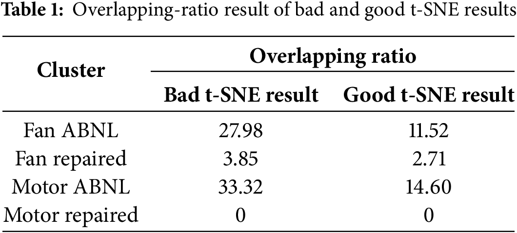
The second step of the index calculation is calculating the proportion of different clusters in each grid. If there is a cluster proportion over 70% in a grid, this grid represents this cluster, and the grid will be labeled as this cluster. If no cluster in this grid has a proportion greater than 70%, that means the proportion in this grid is orderless, which also means this grid does not represent any category, then the grid will be labeled as “orderless”. Regarding threshold setting, we choose 70% because we think the cluster distribution in a grid follows the normal distribution. If a cluster occupies more than 70% of the entire grid data, the grid can be considered statistically equivalent to the cluster. After calculating all grid proportions, the next and final step is calculating the overlapping-ratio between each cluster and orderless data. In the calculation, we tally the total number of grids occupied by each cluster and the number of orderless grids among them. By dividing the latter by the former, we get the overlapping-ratio. We have prepared a Pseudo code to illustrate this complex calculation process, as shown in Appendix A. In determining whether overlapping-ratio qualifies, we consider whether the average ratio of all clusters below 20% is qualified or the t-SNE result is defective. This research uses two t-SNE results, which have already been manually judged, to test the index’s feasibility. Fig. 15 shows the mesh (step 1) and proportion (step 2) calculation results. We can see that the number of orderless (black) grids in bad t-SNE results is more than in good t-SNE results. We can also see that “fan repaired” and “motor repaired” in both bad and good results are separating pretty well; this can be proved with our index. Table 1 shows the overlapping-ratio of all clusters in 2 different results. The index of “fan repaired” and “motor repaired” is pretty small, and the index of “fan ABNL” and “motor ABNL” in the bad result is close to or even over 30, but the index of these 2 clusters in the pleasing result is below 15. This result proves that the overlapping-ratio can identify the “good” or “bad” t-SNE result, and its judgment can fit the manual judgment.

Figure 15: Results about mesh and proportion calculation; (a) bad result judged by a human; (b) good result judged by a human

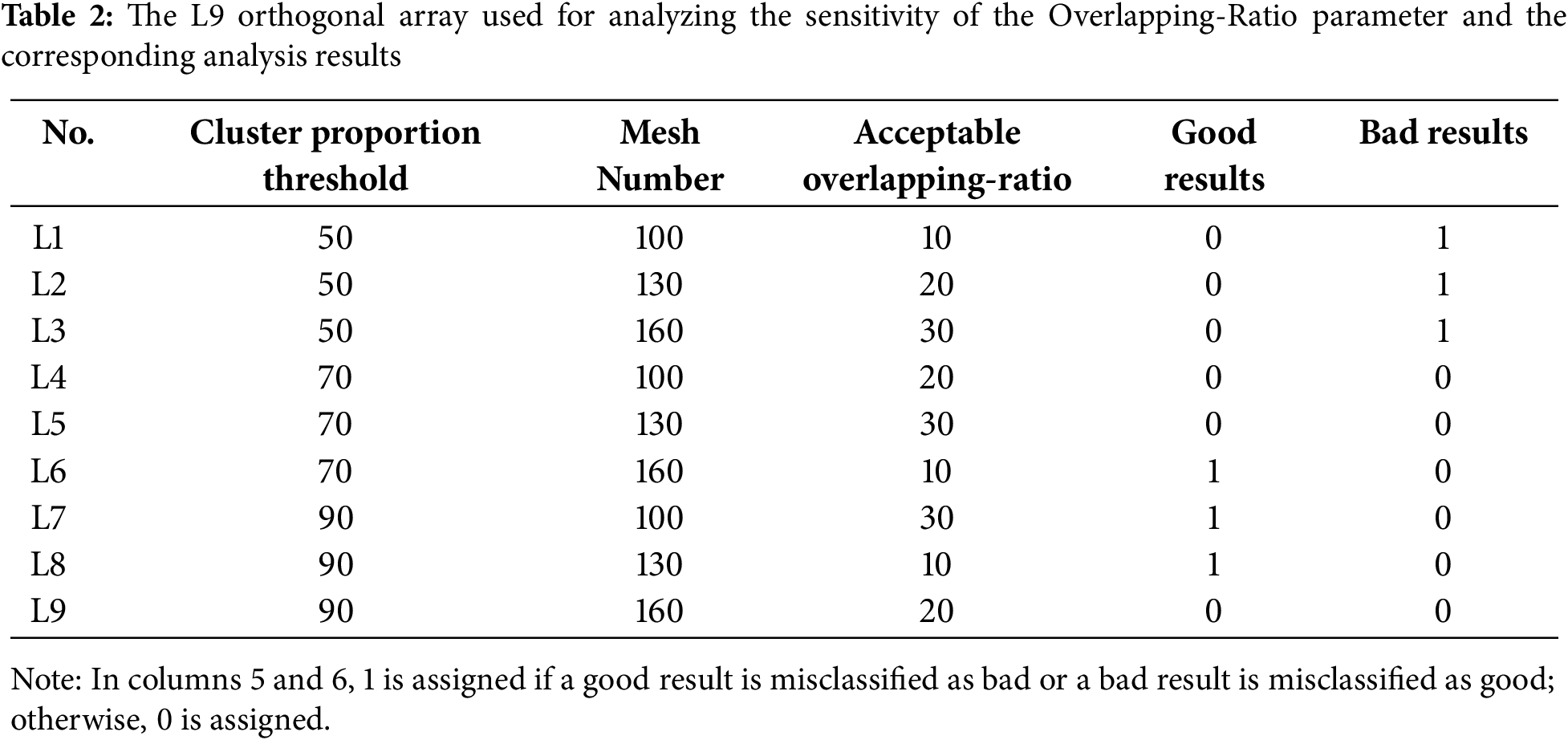
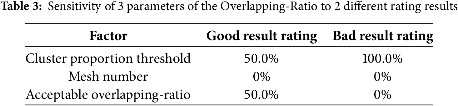
Although the proposed method significantly reduces human intervention in evaluating t-SNE results, specific manually defined threshold values remain in the computation process. Therefore, a sensitivity analysis was conducted on these input parameters to enhance their applicability and reliability in future implementations. Specifically, the Taguchi method was employed for the sensitivity analysis, using an L9 orthogonal array with three factors (cluster proportion threshold, mesh number, and acceptable overlapping-ratio), each at three levels. The analysis focused on two types of misclassification: (1) misclassifying good results as bad, and (2) misclassifying bad results as good. The orthogonal array and corresponding t-SNE evaluation results are presented in Table 2. Following the sensitivity analysis based on Table 2, the results shown in Table 3 reveal that the cluster proportion threshold and acceptable overlapping-ratio each had a 50% sensitivity in identifying good t-SNE results. However, the cluster proportion threshold exhibited a 100% sensitivity in identifying bad t-SNE results. This finding indicates that extreme values of the cluster proportion threshold, either too small or too large, can lead to misjudgments. Therefore, the value of the cluster proportion threshold selected in this study is considered to be appropriate.

3.3.2 Methodology of Calculating the Distributed-Density

Although overlapping-ratio can filter out the cluster-mixed t-SNE result, if the distribution range of a single cluster is too extensive and too sparse, it is also considered disqualified. Hence, in this research, we propose an index called “distributed-density”, which represents each cluster’s distribution pattern. The index calculation here is based on the processed cluster-mesh data in overlapping-ratio calculation, shown in Fig. 15. First, we mark a 3 × 3 grid centered on the target grid and calculate the number of surrounding grids with the same cluster as the target grid. Then, divide the number of the same cluster grids by the number of surrounding grids to get the single grid distributed-density. Finally, the density belonging to each cluster is averaged, resulting in the cluster’s distributed-density. We have organized the calculation process into equations, as shown in Appendix A. For example, Fig. 16 is a 3 × 3 example matrix (M). Here, we use M11 as an example. This grid belongs to cluster 1; there is only one grid with the same cluster around M11, and there are a total of 3 grids around M11. Then, we can calculate M11 density is 1/3 = 33.3%, and there are a total of 4 grids belonging to cluster 1 in the matrix. Their density is [33.3%, 66.7%, 37.5%, 40%]. Hence, the distributed-density of cluster 1 is 44.38%. Due to our calculation method, the density of the grid, which is located at the edge of the cluster, might get a low value. Hence, we believe the density over 60% is a qualified t-SNE result. In our case, we perform distributed-density calculations on the two t-SNE result data in Fig. 15, and the calculation result is shown in Table 4. We can see that “Motor ABNL” in bad results gets a density smaller than 60. That’s because this cluster is scattered across 7 locations, shown in Fig. 17: Seven locations of Motor abnormal conditions. This result proves that our index can identify the cluster’s distribution and rate for it. Although this index seems less critical than overlapping-ratio, we believe that when there is no overlapping in t-SNE results but the same cluster appears in multiple locations, this index can identify such bad t-SNE results. Reduce the possibility of identifying t-SNE results perceived as bad by humans as good outcomes.

Figure 16: Example matrix (M) with 3 × 3 and including 4 clusters (1 to 4)

Figure 17: Seven locations of motor abnormal conditions

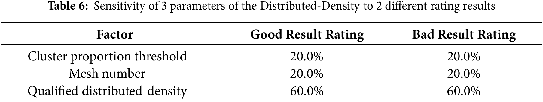
Finally, a sensitivity analysis is performed on the calculation parameters of distributed-density, which is similar to overlapping-ratio. The Taguchi method with an L9 orthogonal array comprising three factors (cluster proportion threshold, mesh number, and qualified distributed-density), each at three levels, was employed again for this analysis. The analysis focused on two types of misclassification: (1) misclassifying good results as bad, and (2) misclassifying bad results as good. The orthogonal array and corresponding t-SNE evaluation results are presented in Table 5. Based on the sensitivity analysis using the data in Table 5, the results are summarized in Table 6. The analysis revealed that cluster proportion threshold and mesh number consistently exhibited low sensitivity (20%) in the classification of good and bad t-SNE results, whereas qualified distributed-density demonstrated the highest sensitivity at 60%. This indicates that only a moderate value of qualified distributed-density can maintain classification accuracy. Therefore, the value of the qualified distributed-density selected in this study is considered appropriate.

3.3.3 The Comparisons between Common Existing Rating Method and the Method Proposed in This Research

The motivation for developing our own t-SNE rating method stems from the suboptimal performance of the evaluation approaches we previously employed. The previous method we used is the Davies-Bouldin Index (DBI). The criteria of DBI are based on intra-cluster similarity and inter-cluster dissimilarity, which is similar to the concept of the rating method we proposed. The lower the DBI, the better the clustering solution. Although there is no absolute threshold, it is commonly accepted that a DBI value below 1 indicates reasonable clustering, while a value below 0.5 suggests good clustering performance. In our research, the DBI value of both good and bad results is bigger than 1, where the bad result is 6.5 and the good result is 4.6. This might be due to the characteristics of DBI. When we address the scenarios where the same class data is distributed across multiple distant regions, which is similar to our good t-SNE result, shown in Fig. 15, DBI fails to provide an accurate assessment. This is because DBI calculates the average within-cluster distance for each cluster. When instances of the same class are distributed across multiple separate regions, the average distance increases, leading to inaccurate evaluation results. To address this issue, we adopted a density-based approach to mitigate the impact of increased distances caused by multi-region distributions, thereby avoiding inaccurate evaluations.

4  Multiple Layers of Neural Network Model for Main Hoisting Motor Failure Detection

There are many methods to propose a failure detection model. In this research, we choose a neural network as the base of the detection model. We know that neural networks comprise hyperparameters such as layers and neurons. The configuration of hyperparameters significantly affects the performance of neural networks. In most cases, these hyperparameters are designed by humans, and this dramatically tests the designer’s experience and patience. This tuning method goes against this study’s goal of minimizing human intervention. Hence, in this research, we use a Bayesian optimizer to design the hyperparameters of the detection model. Details about Hyperparameter Design will be explained in Section 4.1, and we will also explain the details about model training and testing in Section 4.2.

4.1 The Hyperparameter Design of the Motor Failure Detection Model

In the previous section, we mentioned that we were trying to design the hyperparameter without human intervention. Currently, many methods allow machines to adjust hyperparameters automatically, such as the grid search method, random search method, and others. Although these methods are useful, they require substantial computational resources and have the defect of uncertainty in finding the optimal solution. To overcome the above problems, we use a Bayesian optimizer to tune the model hyperparameters. Bayesian optimization was proposed after the 1960s, primarily to address the high computational cost of the function optimization problem. The main idea is to use a surrogate model to approximate the objective function and guide the search for its optimal value. In each iteration, the evaluation of the objective function is used to update the surrogate model, typically modeled using a Gaussian distribution. Here, we take treasure hunting as an example. The treasure is the answer we want. In our case, this is the best hyperparameter we require. The treasure map represents the surrogate model, and the objective function represents the treasure location we aim to discover. When we choose a location and start digging, the result of this digging will be marked on the map and used to recalculate the possible location of the buried treasure until the treasure is found.

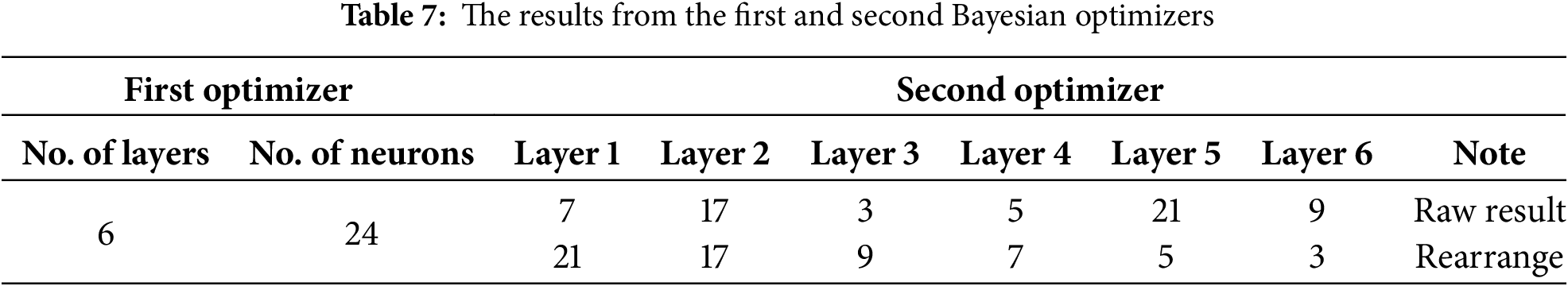
After briefly explaining the working principle of the Bayesian optimizer, we will explain how we use it here. In this research, we use the optimizer to tune the hyperparameter. Although it can significantly reduce computational costs, the numerous combinations of layers and neurons still require a relatively long computation time. Hence, we optimize layers and neurons separately. First, we use an optimizer to search for the best layer number. In the analysis, we set two variables, namely, the number of layers and the number of neurons. During the optimization iterations, the optimizer selects several layers and assigns the same number of neurons to all layers to evaluate this combination’s performance, and the result will be used to do the second optimization. The second optimization focuses on exploring the number of neurons in each layer. In the optimizer settings, the model layers for this optimization are created based on the number of layers resulting from the first optimization, and the number of neurons in each layer will be optimized with the neuron count from the first optimization serving as the upper limit. The result from this optimizer will be the base of our failure detection model. In the optimizing process, both the first and second optimizers underwent 100 iterations. The result of the first optimizer is six layers with 24 neurons, and the second optimizer result is [7,17,3,5,21,9]. To make it more reasonable, in the subsequent training, we rearranged it and used [21,17,9,7,5,3] as the base for the model’s hidden layer. The Bayesian optimizer results are summarized in Table 7.

4.2 Main Hoisting Motor Failure Detection Model Training and Test

In this section, we will explain the motor failure detection model in detail. About model training, benefiting from the hyperparameter tuning process we did in the previous section. We can skip the steps of manually designing and testing hyperparameters and proceed directly to the training step. In the model training setting, the hyperparameter directly adopts the results of the Bayesian optimizer. The model executes 1000 iterations, with the early stopping threshold set to 5, aiming to prevent overfitting. Regarding training data, we randomly select 80% (13,701) from all of the data, and the remaining 20% (3425) is used for testing, which is not included in the training. In every training iteration, 85% (11,646) of the training data is used for model training, and the other 15% (2055) is used for model validation. Fig. 18 shows the validation accuracy of the model we trained. We can see that after the iterations exceed 800, the accuracy remains stable at around 95%. The reason for the accuracy cannot reach 100%. We believe that is because the features of “fan ABNL” and “motor ABNL” are too similar. In Fig. 15b, we can see that most of the orderless data is located between these two clusters. This phenomenon may be caused by the sensor’s installation position. Hence, although the model has a 5% loss, we believe this loss does not significantly affect the model’s performance. Therefore, we will use this model for subsequent testing.

Figure 18: Model training validation accuracy

We used 3425 untrained data to test the model in the testing phase. We tested the model’s overall accuracy and evaluated its accuracy in handling various conditions (clusters). Fig. 19 shows the overall accuracy of the model. The trend of the line is similar to the line in validation accuracy. This is unsurprising because the test and validation data come from the same database, but we discovered something interesting during the process. Fig. 20 shows the accuracy of the model under four conditions. We see that the accuracy of “fan repaired” and “motor repaired” is over 95% and close to 100%, but the accuracy of “fan ABNL” and “motor ABNL” is around 90~95%. We believe this corresponds to the previous words, where we think the two features are too similar. That makes the model a misjudgment in identifying these two conditions. Although there are model misjudgments, the error rate is only 5–10%, which we think is acceptable. We believe this small margin of error may be caused by the sensor itself or its installation position.

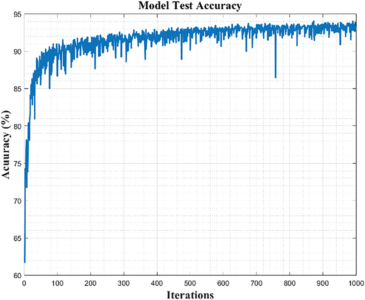
Figure 19: The overall test accuracy of the 1000 iterations motor failure detection model

Figure 20: The test accuracy of the model with 1000 iterations under four different conditions

5  Conclusions

This research aims to explore, analyze, and discuss fault diagnostics methods for the hoist motor of a bridge crane. We propose a novel method using the frequency band t-SNE result and our developed t-SNE result rating method to find the required feature without extensive human intervention. In our case, each component’s normal and abnormal conditions in the crane are properly integrated into the graph and cluster into groups. Normal and abnormal conditions can be easily separated by using a small number of features (bands), but the separation of different abnormal conditions cannot be achieved. Therefore, we compared the two inseparable conditions and identified the bands with the most significant difference between them as an additional feature. As expected, the additionally selected band effectively separates the previously mixed conditions in the t-SNE result. For model training, we used a Bayesian optimizer to search for the model’s hyperparameters, aiming to minimize human intervention. The model trained with the hyperparameters provided by the optimizer and the previously extracted features achieved 95% accuracy in the validation phase and also 95% accuracy in the test phase. During the test phase, we identified why the accuracy could not reach 100%. This was due to the two fault conditions having overly similar features, making it difficult for the model to distinguish them accurately. However, we believe this 5% error does not significantly affect performance. Nevertheless, in future research, we hope to eliminate this 5% error to achieve the model’s optimal decision-making capability.

Acknowledgement: Not applicable.

Funding Statement: This research was funded by National Science and Technology Council, Taiwan, grant numbers 112-2622-E-992-022 and 112-2221-E-992-086. The projects are granted to Tsung-Liang Wu. The URL to sponsor’s website is https://www.nstc.gov.tw/?l=en (accessed on 18 June 2025).

Author Contributions: The authors confirm contribution to the paper as follows: Conceptualization, Tsung-Liang Wu; methodology, Tsung-Liang Wu and Yu-Tang Cao; software, Shin-Hung Lin and Raphael Brent Lau Hundangan; validation, Yu-Tang Cao; formal analysis, Shin-Hung Lin; investigation, Raphael Brent Lau Hundangan; resources, Tsung-Liang Wu; writing—original draft preparation, Shin-Hung Lin; writing—review and editing, Raphael Brent Lau Hundangan and Yu-Tang Cao; visualization, Yu-Tang Cao; supervision, Edward Basaong Ang and Tsung-Liang Wu; project administration, Tsung-Liang Wu; funding acquisition, Tsung-Liang Wu. All authors reviewed the results and approved the final version of the manuscript.

Availability of Data and Materials: Due to the nature of this research, participants of this study did not agree for their data to be shared publicly, so supporting data is not available.

Ethics Approval: Not applicable.

Conflicts of Interest: The authors declare no conflicts of interest to report regarding the present study.

Appendix A

Appendix B Equation of Distributed-Density Calculation in Section 3.3.2

{Ma=MatrixofClusterAMeshresultSCa=MatrixofsinglegriddistributeddensityinMaCa=DistributeddensityofMamesh_num=SettingofMeshnumber(A1)

SCa[i,j]=∑x=i−1i+1∑y=j−1j+1(δ(Ma[i,j],Ma[x,y]))∑x=max(1,i−1)min(mesh_num,i+1)∑y=max(1,j−1)min(mesh_num,j+1)(1),{i>0,i≤mesh_numj>0,j≤mesh_num(A2)

δ=Kronecker   delta⇒δij={0,ifi≠j1,ifi=j(A3)

Ca=∑x=1mesh_num∑y=1mesh_num(Ma[x,y])∑x=1mesh_num∑y=1mesh_num(δ(Ma[x,y],1))(A4)

References

1. Carlo HJ, Vis IFA, Roodbergen KJ. Storage yard operations in container terminals: literature overview, trends, and research directions. Eur J Oper Res. 2014;235(2):412–30. doi:10.1016/j.ejor.2013.10.054. [Google Scholar] [CrossRef]

2. Yan W, Zhu Y, He J. Performance analysis of a new type of automated container terminal. Int J Hybrid Inf Technol. 2014;7(2):237–48. doi:10.14257/ijhit.2014.7.2.22. [Google Scholar] [CrossRef]

3. Zhang J, Wang P, Yan R, Gao RX. Long short-term memory for machine remaining life prediction. J Manuf Syst. 2018;48(3):78–86. doi:10.1016/j.jmsy.2018.05.011. [Google Scholar] [CrossRef]

4. Lee J, Wu F, Zhao W, Ghaffari M, Liao L, Siegel D. Prognostics and health management design for rotary machinery systems—reviews, methodology and applications. Mech Syst Signal Process. 2014;42(1–2):314–34. doi:10.1016/j.ymssp.2013.06.004. [Google Scholar] [CrossRef]

5. Jia F, Lei Y, Lin J, Zhou X, Lu N. Deep neural networks: a promising tool for fault characteristic mining and intelligent diagnosis of rotating machinery with massive data. Mech Syst Signal Process. 2016;72:303–15. doi:10.1016/j.ymssp.2015.10.025. [Google Scholar] [CrossRef]

6. Abboud D, Baudin S, Antoni J, Rémond D, Eltabach M, Sauvage O. The spectral analysis of cyclo-non-stationary signals. Mech Syst Signal Process. 2016;75(5):280–300. doi:10.1016/j.ymssp.2015.09.034. [Google Scholar] [CrossRef]

7. Saidi L, Ali JB, Fnaiech F. Bi-spectrum based-EMD applied to the non-stationary vibration signals for bearing faults diagnosis. ISA Trans. 2014;53(5):1650–60. doi:10.1016/j.isatra.2014.06.002. [Google Scholar] [PubMed] [CrossRef]

8. Kulkarni S, Wadkar SB. Experimental investigation for distributed defects in ball bearing using vibration signature analysis. Procedia Eng. 2016;144(4):781–9. doi:10.1016/j.proeng.2016.05.086. [Google Scholar] [CrossRef]

9. El-Thalji I, Jantunen E. A summary of fault modelling and predictive health monitoring of rolling element bearings. Mech Syst Signal Process. 2015;60(7):252–72. doi:10.1016/j.ymssp.2015.02.008. [Google Scholar] [CrossRef]

10. Prudhom A, Antonino-Daviu J, Razik H, Climente-Alarcon V. Time-frequency vibration analysis for the detection of motor damages caused by bearing currents. Mech Syst Signal Process. 2017;84(1):747–62. doi:10.1016/j.ymssp.2015.12.008. [Google Scholar] [CrossRef]

11. Delgado-Arredondo PA, Morinigo-Sotelo D, Osornio-Rios RA, Avina-Cervantes JG, Rostro-Gonzalez H, de Jesus Romero-Troncoso R. Methodology for fault detection in induction motors via sound and vibration signals. Mech Syst Signal Process. 2017;83(995):568–89. doi:10.1016/j.ymssp.2016.06.032. [Google Scholar] [CrossRef]

12. Shao S, Sun W, Wang P, Gao RX, Yan R. Learning features from vibration signals for induction motor fault diagnosis. In: Proceedings of 2016 International Symposium on Flexible Automation (ISFA); 2016 Aug 1–3; Cleveland, OH, USA. doi:10.1109/isfa.2016.7790138. [Google Scholar] [CrossRef]

13. Tahmasbi D, Shirali H, Sajad Mousavi Nejad Souq S, Eslampanah M. Diagnosis and root cause analysis of bearing failure using vibration analysis techniques. Eng Fail Anal. 2024;158:107954. doi:10.1016/j.engfailanal.2023.107954. [Google Scholar] [CrossRef]

14. Duche R, Sarwade N. Energy efficient fault tolerant sensor node failure detection in WSNs. Int J Eng Technol Innov. 2016;6(3):190–201. [Google Scholar]

15. Jolliffe IT, Cadima J. Principal component analysis: a review and recent developments. Phil Trans R Soc A. 2016;374(2065):20150202. doi:10.1098/rsta.2015.0202. [Google Scholar] [PubMed] [CrossRef]

16. Zhao H, Zheng J, Xu J, Deng W. Fault diagnosis method based on principal component analysis and broad learning system. IEEE Access. 2019;7:99263–72. doi:10.1109/access.2019.2929094. [Google Scholar] [CrossRef]

17. Pule M, Matsebe O, Samikannu R. Application of PCA and SVM in fault detection and diagnosis of bearings with varying speed. Math Probl Eng. 2022;2022(5):5266054. doi:10.1155/2022/5266054. [Google Scholar] [CrossRef]

18. Kumar P, Singh S, Song DY. Investigation of transfer learning method for motor fault detection. Machines. 2025;13(4):329. doi:10.3390/machines13040329. [Google Scholar] [CrossRef]

19. Abdulkareem A, Anyim T, Popoola O, Abubakar J, Ayoade A. Prediction of induction motor faults using machine learning. Heliyon. 2024;11(1):e41493. doi:10.1016/j.heliyon.2024.e41493. [Google Scholar] [PubMed] [CrossRef]

20. Gao T, Yang J, Tang Q. A multi-source domain information fusion network for rotating machinery fault diagnosis under variable operating conditions. Inf Fusion. 2024;106(3):102278. doi:10.1016/j.inffus.2024.102278. [Google Scholar] [CrossRef]

21. Gao T, Yang J, Wang W, Fan X. A domain feature decoupling network for rotating machinery fault diagnosis under unseen operating conditions. Reliab Eng Syst Saf. 2024;252(3):110449. doi:10.1016/j.ress.2024.110449. [Google Scholar] [CrossRef]

22. Lee CY, Lin WC. Induction motor fault classification based on ROC curve and t-SNE. IEEE Access. 2021;9:56330–43. doi:10.1109/access.2021.3072646. [Google Scholar] [CrossRef]

23. Buchaiah S, Shakya P. Bearing fault diagnosis and prognosis using data fusion based feature extraction and feature selection. Measurement. 2022;188(2):110506. doi:10.1016/j.measurement.2021.110506. [Google Scholar] [CrossRef]

24. Wang Z, Wang S, Cheng Y. Fault feature extraction of parallel-axis gearbox based on IDBO-VMD and t-SNE. Appl Sci. 2024;14(1):289. doi:10.3390/app14010289. [Google Scholar] [CrossRef]

25. Van Der Maaten L, Hinton G. Visualizing data using t-SNE. J Mach Learn Res. 2008;9:2579–625. [Google Scholar]